Experiment verification of hologram generation using intensity images Ni Chen, Keehoon Hong, Jiwoon Yeom, Jae-Hyun Jung, and Byoungho Lee* School of Electrical Engineering, Seoul National University Gwanak-Gu Gwanakro 1, Seoul 151-744, Korea ABSTRACT We propose a digital hologram generation method from diffracted intensity images based on the transport of intensity equation. In this paper we do experiment to verify the proposed method with coherent illumination with simple experiment setup using the intensity images capture process. The experiment results show that our proposed method has advantages compared to both the conventional holography with interferometry and the hologram generation based on multiple intensity images. Keywords: Holography, transport of intensity equation, digital holography.
1. INTRODUCTION Optical wavefronts carry the information about an object which reflects or passes the wavefronts. The wavefronts reflect the properties of the object, such as the color, shape, index of refraction, and the thickness. Generally, only the intensity of the wavefront can be detected by the photography detector, while the phase information is lost. Holography is one of the powerful methods for wavefront detection. It records the interferometry of the wavefront and a reference wavefront. This converts the phase information to an intensity modulation. However, the introduction of the reference wave needs a complicated interference experimental setup which also induces some problems in the hologram reconstruction, such as the DC term problem and the twin image problem [1-3]. Another type of wavefront measurement technique is non-interferometry method, like the methods based on the Shack-Hartmann sensor which lacks spatial resolution [4]. Recently, phase retrieval techniques for the full wavefront reconstruction using a simple setup are proceeding. These methods usually use several intensity images to obtain the wavefront. They are mainly based on the variants of the Gerchberg-Saxton (GS) algorithm [5-7], the solution of transport of intensity equation (TIE) [8-10], or the composite of the two methods [11-14]. The GS variant methods always need large amount of intensity images or consume much computer calculation time [16]. The TIE method needs less intensity images but is limited to the near field. Fortunately, the GS method and TIE method can be combined to get the strengths of both of them. These methods are based on the full approximation storage (FAS) [15] method which is not widely used in the wavefront reconstruction.
(a)
(b)
Figure 1. How intensity reflects phase information. *
[email protected]; phone 82 02 880-7245; fax 82 02 873-9953; http://oeqelab.snu.ac.kr/
The evolution of the intensity distribution of an object wave field can be explained by Figure 1(a). Suppose the object is a pure phase object, Iz1 and Iz2 are the intensity images at different planes along the optical axis. The energy flow on the incident field is perpendicular to the phase front, as indicated by the arrows. The intensity of the field is indicated by the density of the arrows and it changes with the propagation. As Figure 1(b) shows, the intensity of a propagating object wavefront can be expressed by
I z Frz U 0 ( x, y, z0 ) , 2
(1)
where Frz{} is the notation of propagation with a distance z. U0(x, y, z0) is the wavefront just after the object and expressed by
U0 A0 exp j ( x, y, z0 ) ,
(2)
where A0 is the amplitude of the wavefront and φ(x, y, z0) is the phase distribution of the object. The intensity distribution of the object is I0=|U0(x, y, z0)|2 . Under Fresnel diffraction, Frz{ U0(x, y, z0)|} is [17]
U (u, v, z )
e jkz jk U 0 ( x, y, z0 ) exp (u x)2 (v y)2 dxdy. j z 2z
(3)
Substituting Eq. (3) to Eq. (1) and discarding the non-linear term which limits Eq. (1) to near-Fresnel region, we can get this linear equation [12]:
I0 (r , z) (r , z) k z I ,
(4)
where▽⊥=(∂x, ∂y) is the two dimensional gradient operator and r⊥ is the vector in the x-y plane and k is the wave number. In the case of I(r⊥, z)>0 in a region with smooth boundary at the x-y plane and φ(r⊥, z) is continuous, the solution is unique [9, 10]. The Fresnel diffraction equation without the phase factor is exactly equal to the TIE. Thus if we know two-dimensional intensity distributions of the object wave at multiple transverse planes, the phase of the object wave can be calculated by solving the TIE. And then, the complex wave field of the object is fully obtained. We proposed a method for generating digital hologram from three diffracted intensity images. Section 2 is the principle of the proposed method and section 3 is the experiment verification.
2. PRINCIPLE 2.1 Capturing process
(a)
(b)
Figure 2. Scheme of the setup for the image capturing using (a) transmission type and (b) reflection type
Figure 2 is the scheme of the image capturing process: Figure 2(a) is for the transmission type and Figure 2(b) is for the reflection type. An object is illuminated by a laser and the object wave is captured by a charge-coupled device (CCD). Three intensity images are captured by the CCD while one is located at the hologram plane and the other two are located after and before the hologram plane with the same gap noted as △z. The three images are noted as IZ0, IZp, and IZn, as Figure 3 shows.
Figure 3. The arrangement of the captured intensity images.
Thus the evolution of the intensity images in Eq.(4) can be expressed as
z I
z z0
I zn I zp 2z
.
(5)
The FAS algorithm is efficient and also applicable even outside the Fresnel region up to and including the Fraunhofer region. Thus we use the FAS algorithm to calculate the phase distribution from Eqs. (1) and (4). The intensity images are sampled with different grid sizes and piled up as a pyramid. Initial solutions for the finer grid are the solutions of the previous coarser grid. Because the TIE works efficient for reconstruction of the low spatial frequency and the GS method works well for the high spatial frequency, we use full mutigrid method (FMG) [15] for solving the TIE in each grid except for the two finest grids. For the two finest grids, we use the previous TIE solution as the initial solution and the GS algorithm with little iteration (generally less than 10).The final result is used as the phase solution of the hologram. The amplitude of the hologram is used as the square root of the intensity Iz0,
A(r , z0 ) I (r , z0 ).
(6)
Thus the complex wave field of the object at the hologram plane is obtained.
3. EXPERIMENT RESULTS 3.1 Experiment
Figure 4. Experiment setup.
We performed an experiment to verify the principle. Figure 4 is the experiment setup. The object we used in the experiment is transparent mode of USAF-1951 test target. The wavelength of the laser is λ=532.8nm. The pixel pitch of the CCD is 4.56um with resolution of 1300×960 pixels. The center intensity image was located at a distance of z0=35mm and the interval △ z between two adjacent intensity images is 10mm. The three captured intensity images are shown in Figure 5.
(a)
(b)
(c)
Figure 5. Captured intensity images at planes with distance of (a) z=25mm, (b) z=35mm, and (c) z= 45mm.
The hologram phase is calculated from the intensity images using one FMG method and 8 iterations for the two finest grids. Figure 6 are the amplitude and phase profile of the calculated hologram: Figure 6(a) is the amplitude and Figure 6(b) is the phase.
(a)
(b)
Figure 6. Hologram: (a) amplitude profile and (b) phase profile.
Using inverse numerical Fresnel propagation from Figure 6 we can obtain the digital reconstructed object field at different planes, as shown in Figure 7. Figure 7(a) is the reconstruction at the object plane. We also get the reconstruction at the same plane only from the amplitude of the hologram, as Figure 7(b) shows. It shows that without the calculated phase information, we cannot get the object reconstruction.
(a)
(b)
Figure 7. Reconstructed images with (a) the hologram, and (b) the amplitude of the hologram.
We also verified the correction of the hologram by comparing the experimentally captured intensity images and the intensity images reconstructed from the hologram.
(a)
(b) Figure 8. Comparison between experimentally captured images and images reconstructed from hologram (a) at z=10mm (b) z=30mm.
The two image in the left column of Figure 8 are the experiment captured intensity images at z=10mm and z=30mm, and the two images in the center column are the images reconstructed from the calculated hologram. The two plot images in the right column are the comparison between the experimentally captured images and the reconstructed images from the hologram along the horizontal center line with 300 pixels. We can see that the experiment images and the reconstructed images are almost the same. The correlation for the images at z=10mm is 97.38% and for the images at z=30mm is 93.35%.
Figure 9. Reconstruction at the twin image position.
In order to verify that no twin image occurs, we reconstructed the hologram at the mirror position of the object plane. Figure 9 is the reconstruction. Compared to the reconstruction at the object plane in Figure 7(a), the twin image reconstruction is blurred, which reflects that the twin image does not occur.
4. CONCLUSION In conclusion, we have proposed and verified a method for generating hologram from only three intensity images. The experimental results demonstrated that this method works reasonably well compared to the conventional holography and the method based on the multiple intensity images. In our method, we do not need complicated setup and multiple intensity images capturing. Also the FAS algorithm in the hologram calculation is efficient with less iteration, thus less computer load. We expect this method can be further studied.
ACKNOWLEDGMENT This work was supported by the Brain Korea 21 Program (Information Technology, Seoul National University).
REFERENCES [1] Gabor, D., “A new microscopic principle,” Nature 161, 777-778 (1948). [2] Leith E. N. and Upatnieks J., “Wavefront reconstruction with continues-tone objects,” J. Opt. Soc. Am. 53, 1377-1381(1963). [3] Kreis T. and Juptner W., “Suppression of the dc term in digital holography,” Opt. Eng. 36, 2357-2360 (1997). [4] Geary J. M., [Introduction to Wavefront Sensors], SPIE. Press, TT18 (1995). [5] Pedrini G., Osten W., and Zhang Y., “Wave-front reconstruction from a sequence of iterferograms recorded at diffrerent planes,” Opt. Lett. 30, 833-835 (2005). [6] Bao P., Zhang F., Pedrini G., and Osten W., “Phase retrieval using multiple illumination wavelength,” Opt. Lett. 33, 309-311 (2008). [7] Bao P., Situ G., Pedrini G., and Osten W., “Lensless phase microscopy using phase retrieval with multiple illumination wavelengths,” Appl. Opt. 51, 5486-5494 (2012). [8] Teague M.R., “Irradiance moments: their propagation and use for unique retrieval of phase,” J. Opt. Soc. Am. 72, 1199-1209 (1982). [9] Gureyev T. E., Roberts A., and Nugenr K. A., “Partially coherent fields, the transport of intensity equation, and the phase uniqueness,” J. Opt. Soc. Am. A. 12, 1942-1946 (1995). [10] Paganin D. and Nugent K. A., “Noninterferometric phase imaging with partially coherent light,” Phys. Rev. Lett. 80, 2586-2589 (1998). [11] Rabadi, W. A., Myler, H. R., and Weeks A. R., “Iterative multiresolution algorithm for image reconstruction from the magnitude of its Fourier transform,” Opt. Eng. 35, 1015-1024 (1996). [12] Gureyev T.E., “Composite techniques for phase retrieval in the Fresnel region,” Opt. Eng. 220, 49-58(2003) [13] Eilenberger F., Minardi S., Pliakis D., and Pertsch T., “Digital holography from shadow graphic phase estimates,” Opt. Lett. 37, 509-511 (2012). [14] Ohneda Y., Baba N., Miura N., and Sakurai T., “Mutiresolution approach to image reconstruction with phasediversity technique,” Opt. Rev. 8, 32-36 (2000). [15] Press W. H., Teukolsky S. A., Vetterling W. T., Flannery B. P., [Numerical Recipes in C: The Art of Scientific Computing], 3rd ed.., Cambridge University Press, Cambridge, Sec. 20.6 (2007). [16] Almoro P., Pedrini G., and Osten W., “Complete wavefront reconstruction using sequential intensity measurement of a volume speckle field,” Appl. Opt. 45, 8596-8605 (2006). [17] Goodman J. W., [Introduction to Fourier optics], 3rd ed., Roberts & Company, Englewood, Colorado (2005).