Paolo Pivato, Luigi Fontana, Luigi Palopoli and Dario Petri. Department of Information Engineering and Computer Science. University of Trento. Via Sommarive ...
Experimental Assessment of a RSS-based Localization Algorithm in Indoor Environment Paolo Pivato, Luigi Fontana, Luigi Palopoli and Dario Petri Department of Information Engineering and Computer Science University of Trento Via Sommarive 14, 38123, Trento, Italy Email: {pivato,palopoli,petri}@disi.unitn.it
Abstract—In this paper we show the results of an experimental assessment of an indoor localization system based on a Wireless Sensor Network. The estimated position of a target node embedded in the monitored environment is obtained by running of the Relative Span Exponentially Weighted Localization (REWL) algorithm, a novel localization procedure recently proposed in the literature. The inputs of the algorithm are the Received Signal Strength (RSS) measurements collected in a real indoor scenario. A description of the developed system and a metrological characterization of the proposed technique is presented in this paper.
I. I NTRODUCTION In the last few years the use of Wireless Sensor Networks has become commonplace in different fields, ranging from environmental monitoring in harsh and hostile areas to precision agriculture, from security and surveillance to medicine and industry and – more recently – home automation and assisted living [1], [2], [3], [4]. A recent indoor application for Wireless Sensor Networks (WSNs) is localization of moving targets. This application is motivated primarily by the low cost of this solution and the lack of effective positioning and tracking systems working inside buildings. Indeed, the Global Positioning System (GPS) solves many localization problems outdoor, where the devices can receive the signals coming from the satellites, but the system is hardly usable indoor. Moreover, the wireless nodes present some advantages in terms of system miniaturization, scalability, quick and easy network development, cost and reduced energy consumption. Most of the proposed localization solutions rely on the Received Signal Strength (RSS) measurements. In fact, the RSS can be used to estimate the distance between the unknown node (called target node) and a number of reference nodes with known coordinates (called anchors or beacons). The location of the target node is then determined by multilateration [5]. Unfortunately, most of the work on RSS-based localization is supported only by simulation results, while some experimental studies prove a potential lack of accuracy of the employed models. This is true especially in indoor environment where the propagation of the radiofrequency signals is subjected to such effects as reflections, multi-path interference and fading, which perturb the relationship between distance and RSS. However RSS-based techniques remain an appealing approach.
978-1-4244-2833-5/10/$25.00 ©2010 IEEE
This is mainly due to the fact that the radio signal strength measurements can be obtained with minimal effort and do not require extra circuitry with remarkable savings in cost and energy consumption of the sensor node. Indeed, most of the WSN transceiver chips have a built-in Received Signal Strength Indicator (RSSI), that provides RSS measurement without any extra cost. With this considerations in mind, we would to gain a deep understanding of the different phenomena affecting RSS measurements. Thus, the purpose of our work is two-fold. First, we propose a rigorous experimental study of a particular localization algorithm that highlights the impact of the different effects on the accuracy of the algorithm. Although the study is carried out for a particular algorithm, we believe the methodology is by a large extent generalizable. The second (longer term) goal is to leverage off the experience gained in the experimental study to develop a second generation of robust RSS-based localization algorithms. We examine this issue by considering the log-normal shadowing path loss model, widely used for indoor wireless channel, and characterize it with respect to the experimental measurement context. Our goal was in this case to identify the channel parameters by a linear regression applying the Least Squares Method over a significant set of measurements. After this characterisation is made, we move on to analysing the accuracy of a novel RSS-based algorithm called REWL. Our rigorous metrological characterization of the RSS measurements in a specific indoor environment allows us to provide an insightful interpretation of the limitations of the algorithm, which can be built upon for future developments. The remainder of this paper is organized as follows. Section II describes the experimental framework, detailing the sensor device used (II-A), the measurement scenario (II-B) and the adopted indoor propagation channel (II-C). In Section III, after a brief overview on localization algorithms (III-A), we outline the localization algorithm used in our experiments (III-B) and provide some preliminary experimental results (III-C). In Section IV we conclude the paper. II. T HE MEASUREMENT CONTEXT A. Sensor device The main component for our experimental set-up is a TelosB wireless sensor node produced by Crossbow Inc. It is an
0 Test points Anchors
50 100 150
Distance [cm]
200 250 300 350 400 450 500 550 600 0
50
100
Fig. 1.
150
200
250
300
350 400 Distance [cm]
450
500
550
600
650
700
Location test points within the room. Fig. 2.
open-source wireless sensing platform, based on TIMSP430 microprocessor and equipped with the IEEE 802.15.4 compliant Chipcon CC2420 radio module. We use this type of sensor node device because of its remarkable popularity in the academic community and of the wealth of software available for the platform. The CC2420 transceiver operates in the 2.4 GHz ISM band and supports 8 discrete transmission power levels: 0 , −1 , −3 , −5 , −7 , −10 , −15 and −25 dBm. The radio chip has a built-in Received Signal Strength Indicator that provides a two’s complement 8 bit digital value, which can be read from the RSSIV AL register. The power Prx (in dBm) received at the RF pins can be obtained directly from the RSSIV AL register value by means of the following equation:
The experimental scenario
where the RSSIOF F SET value was found empirically and approximated to −45 dBm. The antenna is a 2.4 GHz planar inverted-F (PIFA) printed on the dielectric substrate of the circuit board, feed by a coplanar waveguide (CPW). It is located on the border of one of the short sides of the node, which has a rectangular shape. The PIFA design is based on the one of the invertedL antenna, a λ/4 long wire monopole folded with respect to the ground plane. Starting from the idea of the invertedL antenna, the inverted-F is obtained by folding down the top section to be parallel to the ground plane. This solution, besides giving the antenna the F shape and name, improves the 50 Ω coupling with the feeding line. Despite this improvement, we experimentally verified that the antenna radiation pattern is not omnidirectional, in accordance with the manufacturer datasheet.
high and stands upright with the antenna facing upwards. The linoleum floor is divided into 68 test point located on a grid with a resolution of 50 cm. They are represented with circles in Fig. 1. The 12 fixed nodes are hanged on the ceiling, 260 cm high, with the side containing the antenna facing downwards the roof (see Fig. 2). They are represented with squares in Fig. 1. The displacement of the fixed nodes forms a rectangular grid covering all the monitored environment. The system performs the RSS measurements from the messages exchanged between the mobile node and each anchor node. The mobile node sends a ping to the 12 anchor nodes requesting a response. Then each anchor node replies in turn with a message containing the node ID and the transmitted power level. When the mobile node receives a reply message, it measures the signal strength through the built-in Received Signal Strength Indicator (RSSI) and reads the other information contained in the message. The process is repeated several times. All the measured RSS data are sent to the base station, which is connected to a laptop personal computer (PC). Finally the collected RSS values are processed and analyzed to extract statistical information and to evaluate the result of the localization algorithm described in Sec. III-B. In order to minimise the exchange of messages and the energy consumption, data collection and processing should be performed on the sensor node. We made a different choice because using the PC allows for an easier statistical analysis, which is the main purpose of this paper, and a more flexible implementation of different localization algorithms. The measuring process is repeated 30 times for each of the 68 test point locations, resulting in a total amount of 24480 RSS values collected.
B. Measurement scenario and methodology
C. Indoor radio channel propagation model
The experimental test-bed is a rectangular room of size 5.8 m x 4 m, furnished with a couch, a bookcase put on the wall, a table and a settle. Therefore the considered environment well emulates a real ambient living. The system infrastructure is composed of 1 mobile node (the target), 1 base station node (the sink) and 12 fixed nodes (the anchors). The mobile node is set on a dielectric support 50 cm
In order to characterize the indoor propagation channel we assume that the signal strength follows the log-normal shadowing path loss model proposed by Rappaport [6] . This propagation model is widely used in indoor wireless link budget and is given by: � � d (2) + Xσw Prx (d) = P (d0 ) − 10η log d0
Prx = RSSIV AL + RSSIOF F SET
[dBm ]
(1)
where Ptx is the transmission power and K is the attenuation factor at the reference distance d0 . It can be shown that the estimation of the distance obtained by inverting the path loss model given by equation (3) is biased. Let d denote the true distance between mobile and anchor node, and dˆ denote the estimated distance. Applying the law of uncertainty propagation, we obtain that the relative bias of the distance estimator is given by: � �2 1 ln 10 b[ dˆ] ≃ σw 2 (4) d 2 10η while the relative standard deviation results: ln 10 σ[ dˆ] ≃ σw d 10η
(5)
Both these formulas have been validated by simulations not reported here for the sake of conciseness. From (4) and (5) we have: 1 ln 10 b[ dˆ] ≃ σw ˆ 2 10η σ[ d ]
(6)
Considering η ranging between 1 and 4, expression (6) assume values in (0.12 σw , 0.03 σw ). Thus the bias could be significant even for small values of σw . Notice also that the relative standard deviation of the estimated distance increases of about 5% to 20% for each dB of RSS standard uncertainty. Thus any distance estimator based on model (2) is very sensitive to RSS uncertainty. To the best of our knowledge these interesting observations have not been reported in the literature before. D. Channel parameters estimation The data set of RSS measurements, collected as described in Sec. II-B, was used to estimate the channel parameters K and η. The transmission power Ptx was set to −25 dBm in all nodes. We decided to use this power level because we verified that it is the minimal one ensuring a complete coverage of the room. Therefore, it allowed us to strike a good balance between coverage and energy consumption. The reference distance d0 , which is related to the antenna far field region, was set equal to 10 cm. We firstly applied a linear regression – i.e. Least Squares Method (LSM) – on all the 24480 RSS values collected, obtaining K = −17.2 and η = 2.3. The result is shown in Fig. 3, where the dots represent RSS measurements and the solid line refers to the theoretical path loss model derived by the
−60 −63 −66 −69 −72
RSS [dBm]
where d is the transmitter-receiver distance (in m), d0 is a reference distance, η is the path loss exponent – the rate at which the signal decays – and Xσw is a zero-mean Gaussian random variable with variance σw 2 . Prx (d) is the received signal strength and P (d0 ) is the power received at the reference distance (both in dB). An alternative formulation for equation (2) is: � � d + Xσw (3) Prx (d) = Ptx + K − 10η log d0
−75 −78 −81 −84 −87 −90 −93 −96 −99 −102 200
300
400
500
600
700
Log−distance [cm]
Fig. 3. Experimental RSS measurements for all anchors and related LSM model. Model parameters are η = 2.3, K = −17.2, ρ = 0.42, σw = 6 dB
linear regression. In order to determine if the data well fit the derived parameters we computed the correlation coefficient, obtaining ρ = 0.42. Moreover, the standard deviation of the RSS measurements results σw = 6 dB, leading to a relative bias of 17%, and a relative standard deviation of 60%, as provided by (4) and (5) respectively. As a second step, we analyzed the path loss model considering each anchor node individually, while the mobile node is still moved in each of the 68 test points. The channel parameters K and η were estimated for each data set of 2040 collected RSS values by still using the LSM. The diagrams in Fig. 4 and Fig. 5 show the distribution of the RSS measurements, respectively for anchor ID #4 (on the border of one of the long sides of the room) and anchor ID #1 (on one corner of the room), together with the plots of the corresponding theoretical log-normal path loss model. As we can see, the channel model error standard deviation is nearly constant for all the anchors. Conversely, the resulting path loss exponents are very different from each other, being equal to 0.5 for anchor ID #4 and equal to 3.1 for anchor ID #1. The correlation coefficients behave in a similar way, being equal to 0.15 and 0.58 respectively. From this point of view, these anchors represent the worst and the best case respectively. Of course a higher value of the correlation coefficient means that the related anchor carries more information about the unknown distance. We also verified that the 4 anchors located on the corners of the room provided the highest value of the correlation coefficient, thus they can be considered the more informative ones. To the best of our knowledge, no previous work has reported remarkable differences of the channel parameters considering each anchor node singularly. In fact, given the different locations of the anchors, the signal is expected to be not affected by the same reflections, fading and multi-path interference, thus leading to a plain difference in the channel models. III. L OCALIZATION ALGORITHMS A. Overview The localization problem can shortly be formalised as follows. Consider a set of nodes N = {A1 , A2 , . . . , An }.
−63
the target node given by:
−66 −69
m 1 X · pˆ = ai m i=1
−72
RSS [dBm]
−75 −78 −81 −84 −87 −90 −93 −96 −99 −102 200
300
400
500
600
700
Log−distance [cm]
Fig. 4. Experimental RSS measurements for anchor ID #4 and related LSM model. Model parameters are η = 0.5, K = −46.1, ρ = 0.15, σw = 5.8 dB
where m is the cardinality of the subset N of visible anchors. Thus, the assumption made in the CL approach is that all the visible anchors are equally near the target node. Since this assumption is not likely the true situation, in [9] this approach was improved by introducing a function which assigns a greater weight to the anchors closest to the target. The result is the Weighted Centroid Localization (WCL) algorithm, which estimates the position of the target node as:
−63
pˆ =
−66 −69 −72
−78 −81 −84 −87 −90 −93 −96 −99 −102 200
n X
(di−g · ai )
i=1 n X
(8) (di−g )
i=1
−75
RSS [dBm]
(7)
300
400
500
600
700
Log−distance [cm]
Fig. 5. Experimental RSS measurements for anchor ID #1 and related LSM model. Model parameters are η = 3.1, K = −6.7, ρ = 0.58, σw = 5.1 dB
Each node has a fixed and known position (hence the name anchors). In this paper we are interested only in 2-D localization since the third coordinate is assumed to be known. Therefore, the position of an anchor is a 2-tuple ai = (xi , yi ), where xi and yi are evaluated with respect to an origin O. Let p denote the position of a target moving node of unknown coordinates (x, y), and RSSi denote the measured intensity of the signal strength from anchor ai experienced by the target. The objective of a localization algorithm is to identify an estimate pˆ = (ˆ x, yˆ) of the position p given the vector [RSS1 , RSS2 , . . . , RSSn ]. The localization algorithms based on the RSS can be generally divided into two categories: range-based, which use several target-to-anchor distance estimations obtained through the RSS measurements, and range-free, which determine the position of the target node without performing distance estimation [5]. To this latter class belongs the algorithm suggested in [7], that generates the ordered sequence of RSS measurements of the anchor nodes and then examines it to determine the location of the target node. In [8] a range-free solution, called Centroid Localization (CL), is proposed. It approximates the location p of the target node calculating the centroid of the coordinates ai = (xi , yi ) of the anchor nodes for which a connection has been established during the measurement (visible nodes). That is the estimated position of
where di is the distance between the target and the anchor ai , estimated through RSSi . The exponent g > 0 determines the weight of the contribution of each anchor to the location estimation. If g = 0 then pˆ is simply the sample mean of the ai and the WCL reduces to the CL approach. Increasing the value of g causes the anchors to reduce their “attraction” capability with respect to the mobile node, thus increasing the relative weight of the nearest anchors. B. Relative Span Exponentially Weighted Algorithm In our localization experiments we use the recently proposed Relative Span Exponentially Weighted Localization (REWL) algorithm [10]. This algorithm is based on the the WCL method. The weights are obtained by the relative placement of the anchor RSS value within the span of all the RSS values measured by the target node. In the estimation of the target position, the REWL algorithm favours the anchors which are likely to be closer to the target node and therefore exhibiting higher RSS values. This is obtained using a weighting factor λ adapted from the exponentially moving average concept. The estimated target node position is given by
pˆ =
n X
[(1 − λ)RSSmax −RSSi × ai ]
i=1
n X
(9) RSSmax −RSSi
(1 − λ)
i=1
where RSSi is the value of the RSS measured between the target and the anchor node ai , and RSSmax is the maximum value in the span of the RSS values measured by the target node. Suggested values for λ, experimentally determined, range from 0.10 to 0.20 [10]. In fact, assuming the path loss model (2), it can be shown that the REWL algorithm reduces to expression (8), where g ranges between 0.5 and 3.9 when η and λ assume values in (1, 4) and (0.1, 0.2) respectively.
1
12 anchors 4 anchors
200 0.9 0.8 0.7 Probability
[cm]
300
400
500
0.6 0.5 0.4 0.3 0.2 0.1
600 150
250
350
450 [cm]
550
650
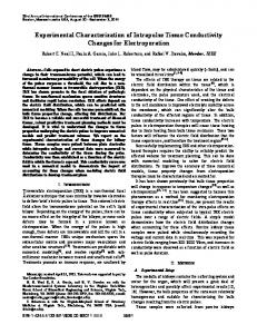
Fig. 6. Estimated and real position of the target node provided by the REWL algorithm with λ = 0.15
0 0
50
100
150 Error [cm]
200
250
300
Fig. 7. Localization error cumulative density functions achieved with the REWL algorithm for λ = 0.1 1
12 anchors 4 anchors
0.9
C. Experimental results
0.8
In Fig. 7, 8 and 9 are reported the cumulative density functions (CDFs) of the localization error resulting from running the REWL algorithm with the 4 anchors on the corners of the room and with all 12 anchor nodes respectively. The values 0.1, 0.15 and 0.2 for the parameter λ have been considered. Clearly, the two lines depicted in each figure are close each other. This is due to the fact that the 4 anchors located on the corners are a subset of all the 12 anchors and, as we previously observed, they carry most of the information about the unknown distance. This imply that the use of only four anchors located near the corners of the considered room could be the best choice for a cost-effective location estimation problem. In particular, the Root Mean Square Error (RMSE) of the distance estimates provided by the algorithm assuming λ = 0.15 ranges between 130 cm to 126 cm passing from 4 to 12 anchors.
0.6 0.5 0.4 0.3 0.2 0.1 0 0
50
100
150 Error [cm]
200
250
300
Fig. 8. Localization error cumulative density functions achieved with the REWL algorithm for λ = 0.15 1
12 anchors 4 anchors
0.9 0.8 0.7 Probability
The diagram in Fig. 6 shows some preliminary results obtained running the REWL algorithm in the scenario described in Section II-B. The dots represent the test points while the squares are the positions estimated by the REWL assuming λ = 0.15. An arrow connect each test point with its corresponding estimated location. As we can see, the algorithm is prone to cluster the estimated positions in the centre of the area delimited by the anchor nodes. This behaviour becomes more noticeable as much as λ increases from 0.10 to 0.20. From a metrological point of view, the measurement repeatability is quite high – the standard deviation is of the order of few cm – but the achieved measurement exhibits a significant bias, which in some positions is even higher than one meter. This occurs because the indoor radio channel is affected by reflections of the signals against the walls, the floor and the ceiling. This situation is even worsen by the presence into the room of furniture with metallic parts, which further perturbs the radio signal propagation. Moreover, some further experiments performed in the same measurement context but in different days provide different values for the estimation bias. This was probably due to external perturbing fields.
Probability
0.7
0.6 0.5 0.4 0.3 0.2 0.1 0 0
50
100
150 Error [cm]
200
250
300
Fig. 9. Localization error cumulative density functions achieved with the REWL algorithm for λ = 0.2
IV. C ONCLUSION In this paper we presented the experimental assessment of a localization system which combines the use of RSSI measurement with a novel localization algorithm proposed in the literature, namely REWL. The system was deployed in a real indoor scenario and, by on-line running of the algorithm, it provided the estimated position of a target node in different test points inside the observation field. The preliminary experimental results shown that the measurement repeatability is quite high but with a significant bias, most likely due to the severe propagation condition of the indoor radio channel.
Also external fields are expected to significantly affect the measurement uncertainty. ACKNOWLEDGMENT This work was performed inside the project ”Acube: Ambient Aware Assistance” funded by the Autonomous Province of Trento, Italy. R EFERENCES [1] I. Akyildiz, W. Su, Y. Sankarasubramaniam, and E. Cayirci, “A survey on sensor networks,” Communications Magazine, IEEE, vol. 40, no. 8, pp. 102–114, Aug 2002. [2] F. Salvadori, M. de Campos, P. Sausen, R. de Camargo, C. Gehrke, C. Rech, M. Spohn, and A. Oliveira, “Monitoring in industrial systems using wireless sensor network with dynamic power management,” Instrumentation and Measurement, IEEE Transactions on, vol. 58, no. 9, pp. 3104–3111, Sept. 2009. [3] A. Carullo, S. Corbellini, M. Parvis, and A. Vallan, “A wireless sensor network for cold-chain monitoring,” Instrumentation and Measurement, IEEE Transactions on, vol. 58, no. 5, pp. 1405–1411, May 2009. [4] Y. Kim, R. Evans, and W. Iversen, “Remote sensing and control of an irrigation system using a distributed wireless sensor network,” Instrumentation and Measurement, IEEE Transactions on, vol. 57, no. 7, pp. 1379–1387, July 2008. [5] H. Liu, H. Darabi, P. Banerjee, and J. Liu, “Survey of wireless indoor positioning techniques and systems,” Systems, Man, and Cybernetics, Part C: Applications and Reviews, IEEE Transactions on, vol. 37, no. 6, pp. 1067–1080, Nov. 2007. [6] T. S. Rappaport, Wireless Communications – Principles and Practice. Upper Saddle River, NJ: Prentice Hall PTR, 1996. [7] K. Yedavalli, B. Krishnamachari, S. Ravula, and B. Srinivasan, “Ecolocation: a sequence based technique for rf localization in wireless sensor networks,” in Information Processing in Sensor Networks, 2005. IPSN 2005. Fourth International Symposium on, April 2005, pp. 285–292. [8] N. Bulusu, J. Heidemann, and D. Estrin, “Gps-less low-cost outdoor localization for very small devices,” Personal Communications, IEEE, vol. 7, no. 5, pp. 28–34, Oct 2000. [9] J. Blumenthal, R. Grossmann, F. Golatowski, and D. Timmermann, “Weighted centroid localization in zigbee-based sensor networks,” in Intelligent Signal Processing, 2007. WISP 2007. IEEE International Symposium on, Oct. 2007, pp. 1–6. [10] C. Laurendeau and M. Barbeau, “Relative span weighted localization of uncooperative nodes in wireless networks,” in Proceedings of the International Conference on Wireless Algorithms, Systems and Applications. WASA 2009, Aug. 2009.