362
IEEE JOURNAL OF OCEANIC ENGINEERING, VOL. 40, NO. 2, APRIL 2015
Modeling, Control, and Experimental Validation of a High-Speed Supercavitating Vehicle David Escobar Sanabria , Gary Balas , Fellow, IEEE, and Roger Arndt
Abstract—Underwater vehicles that travel inside a bubble or supercavity offer possibilities for high-speed and energy-efficient transportation of cargo and personnel. Validation and testing of mathematical models and control systems for these vehicles is a challenge due to the cost and complexity of experimental facilities and testing procedures. A cost-efficient and low-complexity approach to the experimental validation of mathematical models and control systems for a supercavitating test vehicle is presented in this paper. The proposed method enables the testing of control algorithms subject to steady and unsteady flows in a high-speed water tunnel. The method combines a real-time simulation of the vehicle dynamics, force measurements from an experimental scale vehicle, and flight control computer to reproduce the vehicle motion subject to realistic flow conditions and hardware constraints as actuator saturation and time delay. The model of the vehicle dynamics, used for the validation infrastructure and control design, is derived using experimental data. A controller designed to track pitch angle reference commands was tested on the experimental platform. The test cases validated the operation of the vehicle and controller subject to steady and unsteady flows. Index Terms—Controller validation, high-speed underwater vehicles, hybrid simulation, supercavitation.
I. INTRODUCTION
A
N underwater vehicle that travels inside a bubble or supercavity is referred to as a high-speed supercavitating vehicle (HSSV). An HSSV is able to decrease drag and increase speed due to reduction of the contact area between the vehicle and fluid when the supercavity is established [1]–[3]. As a result of the fluid–vehicle isolation, an HSSV also attenuates force oscillations due to flow perturbations. The supercavity is created at a sharp disk cavitator located at the nose of the vehicle. The motion of the HSSV depends upon the forces and moments generated by the cavitator, fins, thrust, gravitational acceleration, and planing generated when the aft end of the vehicle pierces the bubble. Manuscript received January 08, 2013; revised October 31, 2013 and January 18, 2014; accepted March 14, 2014. Date of publication May 05, 2014; date of current version April 10, 2015. This work was supported by the U.S. Office of Naval Research (ONR) under Contract N00014-12-1-0058, Project title: “Development of Control Strategies for Very High Speed Cavity-Running Bodies: Simulations and Small-Scale Experiments.” Dr. R. Joslin is the contract monitor. Associate Editor: F. Hover. D. Escobar Sanabria and G. Balas are with the Department of Aerospace Engineering and Mechanics, University of Minnesota, Minneapolis, MN 55455 USA (e-mail:
[email protected];
[email protected]). R. Arndt is with the Saint Anthony Falls Laboratory, University of Minnesota, Minneapolis, MN 55414 USA (e-mail:
[email protected]). Color versions of one or more of the figures in this paper are available online at http://ieeexplore.ieee.org. Digital Object Identifier 10.1109/JOE.2014.2312591
Fig. 1. Supercavitating test vehicle at SAFL high-speed water tunnel.
Mathematical models and control strategies for supercavitating vehicles have been presented in the open literature; for example, papers [3]–[7] propose control strategies for a vehicle based on idealized models of the vehicle dynamics and supercavity. The experimental validation of mathematical models and control systems for an HSSV is, however, lacking. The validation of an HSSV in realistic flow conditions is relevant to understand the accuracy of the idealized models of the vehicle dynamics and controllers. Another aspect that has not been addressed in the literature is the effect of unsteady flow on the vehicle motion. The goal of this paper is twofold. The first objective is to present a mathematical model of the vehicle dynamics that is validated using experimental data collected in the high-speed water tunnel located at the St. Anthony Falls Laboratory (SAFL), University of Minnesota, Minneapolis, MN, USA. A supercavitating vehicle that consists of a cylindrical body, a disk cavitator, and two wedge swept fins is considered. The considered vehicle is shown in Fig. 1. Special attention to the cavitator forces is given because their interpretation is sometimes inaccurate in the literature. The effect of flow perturbations on the vehicle dynamics is also described and experimentally validated using an oscillating foil that generates unsteady flows in the high-speed water tunnel. Planing forces are not considered in the model of the vehicle dynamics. The second objective of this paper is to present a cost-efficient and low-complexity experimental approach to validate control algorithms and mathematical models for a supercavitating vehicle prototype subject to steady and unsteady flows. The proposed control validation framework is based on hybrid simulation or hybrid testing, a method that combines real-time numerical simulation and measurements of physical variables to evaluate the operation of a dynamical system. This methodology has been successfully used in structural engineering to evaluate the dynamic response of structures [8], [9]. Hybrid testing enables
0364-9059 © 2014 IEEE. Personal use is permitted, but republication/redistribution requires IEEE permission. See http://www.ieee.org/publications_standards/publications/rights/index.html for more information.
SANABRIA et al.: MODELING, CONTROL, AND EXPERIMENTAL VALIDATION OF A HIGH-SPEED SUPERCAVITATING VEHICLE
the evaluation of physical components of a dynamical system in realistic scenarios. The proposed hybrid simulation is intended to evaluate the control systems of a supercavitating vehicle subject to realistic flow conditions and physical constraints as actuator saturation, time delay, measurement noise, and modeling uncertainty. The motion of the supercavitating vehicle is reproduced via realtime numerical simulation of the vehicle dynamics and measurements of the forces applied to a static scale vehicle. The control algorithms, executed on a real-time embedded system, command the cavitator and fin deflections of the experimental vehicle to drive the simulated vehicle motion. The proposed hybrid simulation can be seen as an extension of a hardware-inthe-loop system. Hardware-in-the-loop simulation is a method extensively used in the aerospace, automotive, and robotic industries to reduce costs and time associated with the validation of embedded control systems and actuation systems [10]. The proposed hybrid system enables the validation and testing of embedded controllers and actuation systems for a supercavitating vehicle, but also provides the benefit of capturing the complex interaction between the experimental vehicle, supercavity, and surrounding fluid. A control law designed via an optimization [11], [12] was tested using the hybrid simulation. Its objective is to track pitch angle reference commands subject to steady and unsteady flows. Experimental results demonstrate that the control law is robust to operation in steady and unsteady flows and subject to realistic hardware constraints. The hybrid simulation also demonstrates to be a suitable tool for the iterative validation and testing of software implemented in the real-time embedded computer of the vehicle. The paper is organized as follows. Section II describes the experimental facilities used to derive the model of the vehicle dynamics and construct the proposed validation infrastructure. The mathematical model of the vehicle dynamics, validated with experimental data, is presented in Section III. The proposed hybrid method for the validation of controllers for a supercavitating vehicle is described in Section IV. An example of a controller for the vehicle and experimental test cases executed using the hybrid simulator are presented in Section V. Conclusions and future directions are discussed in Section VI.
363
Fig. 2. Schematic of test section, experimental vehicle, and oscillating hydrofoil (gust generator).
ventilated supercavities. The test vehicle is a cylinder of 50-mm diameter and 210-mm length with a disk cavitator of 40-mm diameter and two lateral fins. The fins are 15 half-angle wedge shaped and 35 swept. The fins have a chord 20 mm and height 35 mm. The tip-to-tip distance of the fins is 114 mm. The fins and cavitator are capable of rotating 10 about their axis of rotation. The back end of the test vehicle is attached to a six-degree-of-freedom force and torque transducer. The transducer is attached to the water tunnel through a strut. An oscillating foil system is used to study the effect of perturbed flow on the forces applied to the test vehicle. The disturbance generation system has the ability to create a 2-D upstream gust. The work in [13] provides a baseline for the design of this system. The test vehicle is placed downstream the gust generator. Fig. 2 shows a schematic of the test section, gust generator, and scale vehicle. III. SUPERCAVITATING VEHICLE MODEL This section presents the mathematical model of a supercavitating vehicle in the longitudinal plane. A brief introduction to supercavitation is presented in III-A. Section III-B presents the coordinate frames used to describe the vehicle dynamics. The generalized equations of motion of the HSSV are presented in Section III-C. Mathematical models of the cavitator and fin forces are described in Sections III-D and III-E, respectively. The effect of flow perturbations on the forces applied to the vehicle is addressed in Section III-F. The equilibrium conditions and linear dynamics of the vehicle are presented in Sections III-G and III-H. A. Supercavitation
II. EXPERIMENTAL FACILITIES
Supercavitation occurs when a sustained large bubble or supercavity is created inside a liquid as a result of a drop in the fluid pressure [2], [3]. The cavitation number
The mathematical models of the HSSV motion and controller validation methods are developed using the experimental facilities at SAFL. The SAFL high-speed water tunnel is a recirculating, closed circuit facility capable of regulating absolute pressures and achieving speeds up to 20 m/s. The test section is 0.19 m (width) by 0.19 m (height) by 1 m (length). A large gas collector dome removes large amounts of air during experiments. The dome enables ventilation experiments to be carried out for long periods of time without recirculation of gas-saturated water [2]. The speed of the water tunnel is calibrated via a laser Doppler velocimetry (LDV) system. The supercavitating scale vehicle shown in Fig. 1 is used for vehicle modeling and controller validation. This vehicle is equipped with a ventilation system that enables the formation of
is a parameter that describes supercavitation. (Pa) is the pressure outside the supercavity, (Pa) is the pressure inside the supercavity, (kg/m ) is the fluid density, and (m/s) is the relative velocity between the flow and the cavitator center of pressure (c.p.). In open waters, supercavitation is typically defined as . The cavitation number can be lowered and supercavitation achieved by either increasing or by decreasing the difference . Injecting air near the nose of the vehicle increases and allows for the formation of ventilated supercavities. Ventilated supercavitation is used to form supercavities
364
IEEE JOURNAL OF OCEANIC ENGINEERING, VOL. 40, NO. 2, APRIL 2015
Fig. 3. Schematic of HSSV with coordinate frames, angles, and distances.
the forces and the moment generated by the cavitator; , , and are the forces and the moment generated by the fins; is the force generated by the thrust; and and are the forces generated by the gravitational acceleration. The forces are defined in the body frame and expressed in newtons (N). The nonlinear equations of motion of the nonplaning supercavitating vehicle are constructed by combining the generalized equations of motion given by (1)–(3) with the description of gravitational forces given in (4) and the cavitator and fin force models described in is the force needed Sections III-D and III-E, respectively. to achieve equilibrium at velocity . The nonlinear vehicle dynamics are used to simulate the vehicle motion and assess when simplified approximations of the vehicle dynamics are valid.
Fig. 4. Diagram of forces at the cavitator.
D. Cavitator Forces at low speeds until reaching natural supercavitation at higher speeds. B. Coordinate Frames and Angles The coordinate frames used to describe the motion of an HSSV are depicted in Fig. 3. The cavitator frame is attached to the cavitator control surface, and its axis is always normal to the cavitator surface and forms an angle with the centerline of the HSSV body. is referred to as cavitator deflection. The cavitator velocity frame is attached to the cavitator c.p. velocity vector . axis forms an angle with . is referred to as cavitator angle of attack. The fin frame is attached to the fin control surfaces, and its axis forms an angle with the centerline of the HSSV body. is referred to as fin deflection. The fin velocity frame is attached to the fin c.p. velocity vector . axis forms an angle with . is referred to as fin angle of attack. The body frame is attached to HSSV body center of gravity (c.g.), and the axis is tied to the body's centerline. The vehicle equations of motion are written with respect to the body frame. Angles are positive in the clockwise direction to respect the right-handed coordinate notation.
The cavitator surface is always in contact with the fluid and is primarily responsible for the drag developed by the HSSV. This control surface rotates about a pivot located at a distance from the HSSV c.g. The cavitator is a sharp disk of area . According to Logvinovich [7], the tangential hydrodynamic forces acting on the disk cavitator surface are negligible; therefore, the only significant force is always normal to the cavitator surface and applied at the c.p., which is the geometric center of the disk. In other words, the cavitator net force coincides with the cavitator axis . The net force at the cavitator along is
This expression is valid for cavitator angles of attack between 45 and 45 . is the cavitator drag coefficient. In free flow . is the drag force coefficient at zero angle of attack and zero cavitation number [14]. is the magnitude of vector . The projections of the cavitator net force (always parallel to ) on the vehicle body axes and are simply
(5)
C. Longitudinal Vehicle Dynamics The generalized longitudinal equations of motion of a nonplaning HSSV are as follows: (1) (2)
(6) (See Fig. 4.) The pitch moment about body axis is given in
generated by the cavitator
(3) (7) (rad/s ) is the angular acceleration about ; (m/s ), (m/s ), (m/s), and (m/s) are the accelerations and speeds along and ; (kg) and (kg m ) are the vehicle mass and moment of inertia about ; , , and are
The moment generated by the cavitator due to displacements of the c.p. is significantly smaller than the pitch moment ; therefore, it is neglected. The force models given in (5) and (6)
SANABRIA et al.: MODELING, CONTROL, AND EXPERIMENTAL VALIDATION OF A HIGH-SPEED SUPERCAVITATING VEHICLE
365
vibrations and unsteadiness. The experimental coefficients and , fitted to polynomials via least squares, have the form and The predictions by Logvinovich
coincide with the experimental data for
Fig. 5. Cavitator force coefficients versus cavitator deflection.
are valid for an unconstrained moving vehicle, whose cavitator velocity and cavitator attack angle are given by (8) (9)
Note that the force measurements follow the Logvinovich prediction of static forces for frequencies up to 2 Hz. This suggests that the motion of the cavitator can be described by the static force models for frequencies up to 2 Hz and a cavitator speed of 4.4 m/s. E. Fin Forces
Expressions (5) and (6) show that for small values of and the cavitator forces applied to the vehicle depend only on the cavitator deflection , but not on the cavitator attack angle . Note that only when
The HSSV models used to describe the vehicle dynamics in [3], [4], [15], and [16] are based on the assumption that for a disk cavitator and small angles
The fins are control surfaces located at the aft end of the vehicle that provide damping and lift for trimming the vehicle motion. Wedge swept fins with span , chord , and fin area are considered. Fins are located at a distance from the vehicle c.g. Experimental and simulation studies on wedge fins piercing the main supercavity of an HSSV have shown that the lift curve is a function of the fin angle of attack , fin immersion , and flow regime [17]. In this paper, it is assumed that the suction side of the fin is fully wetted with a constant immersion. The drag and lift force models, obtained via experimental data, are as follows: (10)
which implies that is a function of , , and variations of due to flow perturbations. The last assumption is not accurate and can lead to dynamic models that do not accurately represent the vehicle motion. The experimental data presented in Fig. 8 demonstrate that does not depend on variations of generated by flow perturbations. The independence of on for small values of suggests that the cavitator motion is not subject to damping. Small angles satisfy and . Angles up to 20 are assumed to follow the small angle approximation. Fig. 5 shows the nondimensional forces and
along and as a function of for both experimental data and Logvinovich models. The experimental data are obtained by deflecting the cavitator of the test vehicle described in Section II at frequencies from 0.25 to 2 Hz at a water speed of 4.4 m/s. The data show error bars associated with the mean value and standard deviation of measurements at different angles . The deviations from the mean values are due to hydrodynamic
(11) Notice that drag and lift forces are expressed along the fin veand , respectively. locity axes and are the fin coefficients of drag and lift, respectively. The drag force at zero fin angle of attack is neglected because it does not significantly affect the vehicle dynamics. The moment generated by displacements of the fin c.p. is assumed to be zero because it is significantly smaller than moments about generated by forces at the cavitator and fins. The coefficients of drag and lift include the forces of the two lateral fins mounted on the vehicle. Fig. 6 shows the lift and drag coefficients from experimental data and models given by (10) and (11). The experimental data were collected by deflecting the fin at frequencies from 0.25 to 2 Hz at a water speed of 3 m/s. Note that the mathematical models of the fin forces accurately match the data of unsteady forces for frequencies up to 2 Hz. The fin forces expressed in the body axes are given in (12)
366
IEEE JOURNAL OF OCEANIC ENGINEERING, VOL. 40, NO. 2, APRIL 2015
Fig. 6. Fin lift and drag coefficients versus fin angle of attack.
The moment about
is given in (13)
The angle from
to
Fig. 7. Forces along HSSV body axes tions. Water mean speed is 3.8 m/s.
and
produced by flow perturba-
is
Equation (12) is valid for a moving unconstrained vehicle as the fin velocity and angle of attack are functions of the vehicle velocities, pitch rate, and fin deflection. The fin velocity vector expressed in the body frame and fin angle of attack for a moving vehicle are as follows: (14) (15)
F. Flow Perturbations
Fig. 8. Forces at the cavitator and fins along bations when the supercavity is established.
axis produced by flow pertur-
An underwater vehicle traveling in the proximity of the sea surface is subject to unsteady flows generated by ocean waves. The effect of waves is most prominent near the sea surface and negligible at large depths [18], [19]. The objective of this section is to show the effect of flow perturbations on the forces applied to a supercavitating vehicle. Section III-F1 shows that supercavition partially isolates force oscillations generated by unsteady flows. Section III-F2 demonstrates via experimental data that variations in cavitator attack angle due to flow perturbations have a negligible effect on the forces at the cavitator along the normal axis of the vehicle. 1) Disturbance Isolation: Flow perturbations vary the angle of attack and forces observed by an underwater vehicle. Fully wetted vehicles are prone to higher force variations than vehicles enveloped with a supercavity due to larger contact area between the vehicle and the fluid. The isolation of disturbances due to supercavitation is demonstrated with an experiment. The gust generator described in Section II was activated at 2 Hz, and forces applied to the experimental vehicle were measured. Fig. 7 shows experimental data of forces along the vehicle body axes and produced by oscillations of the gust generator. Low-frequency components of the force measurements are filtered to eliminate drifts. At 17 s, the supercavity is formed and
forces are attenuated by 75%. The force attenuation demonstrates that supercavitation is a natural mechanism to isolate hydrodynamic disturbances. Although the presence of the supercavity reduces the force oscillations observed by an underwater vehicle due to unsteady flows, the remaining oscillations should be still considered for control design. 2) Unsteady Flow Effect: The data from the experiment presented in Fig. 7 are used to determine the forces at the cavitator and fins due to flow perturbations when the supercavity is established. Force oscillations along at the cavitator and fins are shown in Fig. 8. Forces along are relevant because they generate the vehicle pitching moments and drive the vehicle dynamics. As predicted in Section III-D by (6), forces variations generated by the disk cavitator along due to small variations of attack angle are negligible. Force oscillations generated by small variations in the fin angle of attack are not negligible. As a result, one can model perturbed flow as small force perturbations at the fins, or, equivalently, as small perturbations to . Note that perturbing is equivalent to perturbing . See (15). The forces at the cavitator and fins cannot be directly measured since the experimental scale vehicle is equipped with only
SANABRIA et al.: MODELING, CONTROL, AND EXPERIMENTAL VALIDATION OF A HIGH-SPEED SUPERCAVITATING VEHICLE
a force transducer attached to the vehicle back end. The forces along at the cavitator and fin c.p. , are computed using the following relationship:
367
(24)
(16) and are the force and the moment at the transducer. and are the distances from the center of the transducer to the cavitator and fin c.p. Displacements of the c.p. are much smaller than and . Thus, and are assumed constant. G. Equilibrium for a Conditions of equilibrium vehicle traveling at zero normal velocity , axial velocity , and pitch angle are presented in
(17) (18) (19) The total deflections of the control surfaces are given by the deflections for equilibrium ( and ) added with the deflections for control ( and ), i.e., and H. Linear Equations of Motion A linear model of the longitudinal vehicle dynamics is presented as follows: (20)
(21)
(22)
(23)
(25) The state vector is . The vehicle states are assumed to have small variations , , , and from initial conditions , , , and , respectively. Recall that and are the forces along produced by cavitator and fin deflections, respectively. captures the effect of cavitator deflections, and captures the effect of both fin deflections and flow perturbations. The form of the linear equations of motion is useful to introduce the hybrid simulation described in Section IV. IV. HYBRID SIMULATION The SAFL high-speed water tunnel and experimental facilities used for the hydrodynamic modeling of the supercavitating vehicle can also be utilized to validate the controllers of the vehicle in realistic flow conditions. The proposed validation method is inspired by hybrid simulation. Hybrid simulation combines real-time simulations and measurements of physical variables to test specific parts of a complex system in realistic scenarios. Hybrid simulation is applied to the validation of control systems for a supercavitating vehicle subject to steady and unsteady flows and constraints as actuator saturation, time delay, measurement noise, and modeling uncertainty. The proposed simulator is depicted in Fig. 9. The hybrid simulation of the supercavitating vehicle reproduces the vehicle linear dynamics presented in Section III. The linear dynamics equation
is an approximation of the nonlinear dynamics for which the forces and moments due to cavitator and fin deflections are independent of forces and moments due to vehicle motion. Measurements of and from an experimental static vehicle are combined with the simulation of the forces and moments due to the vehicle motion ( and ) to create a hybrid representation of the linear vehicle dynamics. The linear model of the vehicle dynamics and hybrid dynamics are accurate representations of the nonlinear dynamics for small perturbations of the vehicle states around equilibrium. The static test vehicle, described in Section II, is used as the experimental vehicle in the hybrid test system. The vehicle is attached to a force transducer that measures applied forces and moments. Real-time force measurements from the force transducer and expressions in (16) are used to compute the normal forces along at the cavitator and fins. The normal forces at the control surfaces and are used to propagate the
368
IEEE JOURNAL OF OCEANIC ENGINEERING, VOL. 40, NO. 2, APRIL 2015
Fig. 9. Schematic of the proposed hybrid simulation.
states of the vehicle via numerical integration of the linear dynamics equation. A real-time simulation computer carries out the numerical integration of the dynamics equation to compute the vehicle state vector . The vehicle states are transmitted to the vehicle flight computer, which executes the control algorithms in real time. The control algorithms use the vehicle state information to command the cavitator and fin deflection, which vary the forces applied to the test vehicle and drive the simulated vehicle motion. The terms of the linear dynamics equation ( , , and ) are fully captured with the hybrid simulation. The inertial forces and moments capture the linear and angular accelerations of the simulated vehicle body. is the contribution of the simulated velocities, pitch rate, and pitch angle to the forces and moments applied to the simulated vehicle. Note that captures the variations in fin attack angle and direction of the gravitational acceleration in the body frame. captures the forces and moments due to the cavitator and fin deflections as well as flow perturbations. The real-time force measurements and are the connection between the real world and the numerical simulation. The states of the vehicle are computed by solving the integral equation given by
(26) in discrete time. The solution of the integral equation is performed in real time using a simulation computer. A discussion
about numerical integration of ordinary differential equations is presented in [20] and [21]. The hybrid simulations are performed in the presence of steady and unsteady flows. Unsteady flows are generated using the gust generator described in Section II. The ability of the vehicle controller to attenuate flow perturbations can be evaluated at different frequencies and amplitudes. A particular characteristic of the hybrid simulation is the flexibility to reproduce a variety of vehicle configurations. The mass , vehicle inertia , initial pitch angle , and position of the c.g. described by and can be arbitrarily chosen. The hybrid simulation requires agreement between simulation and measurements; therefore, the initial axial velocity should be the velocity of the water tunnel and , , , and should be the same in both simulation and experimental setup. The proposed hybrid simulation has some limitations. The system is based on the linear vehicle dynamics that consider small perturbations around equilibrium; hence, maneuvers that significantly deviate from the trim condition do not accurately represent the dynamics of the unconstrained vehicle. The effect of propulsion is also not experimentally captured. Variations of fin immersion due to the relative motion between vehicle and supercavity are not fully captured by the hybrid simulation since the test vehicle does not move. Nevertheless, fin immersion variations are expected to be small in the longitudinal plane for the considered perturbations around equilibrium. Planing has not been considered in the proposed approach; however, the hybrid simulation can be adapted to operate, subject to planing forces. For example, large cavitator attack angles, generated by rotations of the gust generator hydrofoils, lead to deflections of the supercavity for which the aft end of the vehicle pierces the bubble. The magnitude of the cavitator attack angles needed to achieve planing depends on the size of the bubble and vehicle. The hybrid system can be also adapted to capture variable velocity in both the water tunnel and dynamics simulation. Thus, control algorithms that use vehicle speed information to improve the performance can be evaluated using the hybrid simulation. V. CONTROLLER VALIDATION EXAMPLE An example is constructed to evaluate the performance of a controller using the hybrid simulation infrastructure. The controller is designed to track pitch angle reference commands and reject disturbances generated by unsteady flows. Although both cavitator and fins can be used for the HSSV control, only the cavitator is used. The models of the vehicle dynamics, actuator, and time delay used for control synthesis are presented in Section V-A. The control law to be tested on the hybrid simulation is described in Section V-B. Section V-C presents the experimental test cases executed with the hybrid simulation and controller. The results of the hybrid simulation are discussed in Section V-D. A. System Components The models of the vehicle dynamics, time delay, and cavitator actuation used for control synthesis are described in the following sections.
SANABRIA et al.: MODELING, CONTROL, AND EXPERIMENTAL VALIDATION OF A HIGH-SPEED SUPERCAVITATING VEHICLE
1) Vehicle Dynamics: The vehicle dynamics are described by the following parameters: 1000 kg/m , 2 kg, 0.0077 kg m , 0.0900 m, 0.0793 m, 0.02 m, m , 0.035 m, 0.02 m, m , , , 0 rad, and 4.39 m/s. Parameters , , , , and were arbitrarily selected. The values of , , and are matched with the cavitator area, fin area, and velocity of the water tunnel to properly combine measurements and simulation. 2) Time Delay: The processing time of the electronics and communication among the simulation computer, embedded control computer, and sensors result in a time delay of the closed-loop interconnection. The total time delay of the hybrid simulation implemented in this work is 0.1 s. A transfer function approximation of the time delay, used for control synthesis, is given in (27) See [22] for details. The Laplace variable is denoted as . The time delay of 0.1 s limits the bandwidth of the closed-loop system with any controller. An approximate upper bound on the maximum bandwidth of the closed-loop system is rad/s (1.6 Hz) [22]. 3) Actuation: The model of the cavitator actuation, composed of the servo–actuator attached to the cavitator, is obtained using system identification techniques. An autoregressive with external input estimator (ARX) [24] model is derived from experimental data. The continuous time transfer function of the cavitator actuation is presented in (28) is the cavitator deflection reference command, and actual cavitator deflection.
is the
B. Controller Synthesis The overall objectives of the control system are tracking of pitch angle step commands with zero error, rejecting disturbances generated by unsteady flows, respecting the cavitator maximum deflection and angular rate, and maximizing the bandwidth for tracking and disturbance rejection. Recall that the time delay of the closed-loop interconnection imposes an upper limit to the system bandwidth of 1.6 Hz approximately. The controller is expected to attenuate disturbances up to 0.7 Hz, which is a realistic requirement given the system limitations due to the time delay and actuation. The states used for feedback are pitch angle (rad) and pitch rate (rad/s). A cascade control structure is adopted in this paper. This structure enables effective disturbance rejection in the inner loop. Fig. 10 shows a schematic of the closed-loop system that integrates the HSSV dynamics , cavitator actuation dynamics Act, inner-loop, and outer-loop controllers and , and time delay of the interconnection Del. is the transfer function from cavitator deflection to pitch rate. The pitch angle and pitch rate reference commands are and . The output disturbance captures
369
Fig. 10. Closed-loop interconnection with inner-loop and outer-loop controllers.
the effect of flow perturbations (variations in the fin angle of attack). In principle, any classical method for the synthesis of singleinput–single-output systems can be applied to design . mixed sensitivity synthesis is used to design the inner-loop controller because specifications on tracking performance, actuator effort, noise rejection, and robustness can be explicitly and simultaneously included into the synthesis framework [11], [12]. The specific objectives of the inner-loop controller include tracking pitch rate commands with errors less than 5% at zero frequency, filtering of noise in the pitch rate measurements at frequencies higher than 6 Hz, rejecting disturbances at frequencies up to 0.7 Hz, and providing gain and phase margins greater than 2 (6 dB) and 45 , respectively. The controller is synthesized using the Matlab Robust Control Toolbox [12]. The state–space representation of the control law in a numerical form is presented in the Appendix. Fig. 11 shows the variations with frequency of the magnitude of the transfer function from pitch reference to tracking error , equivalent to the transfer function from disturbance to pitch rate that is referred to as the sensitivity transfer function . The gain of at low frequency is below the horizontal black dashed line equal to 0.04 ( 28 dB). This indicates that the tracking error is lower than 4% and disturbance attenuation is greater than 96% at low frequency. The magnitude of is bounded by a factor of 2.5 (7.95 dB) at all frequency. This is an indication of good stability margins. In fact, the gain and phase margins of the transfer function from to are 2.2 (7.7 dB) and 67 , respectively. The frequency at which crosses 1 (0 dB) is 0.73 Hz (4.59 rad/s), and, hence, perturbations at frequencies greater than 0.73 Hz are not attenuated by the controller . In addition, pitch rate commands at frequencies greater than 0.73 Hz result in tracking errors greater than the magnitude of . Note that the tracking and disturbance rejection characteristics of the closed-loop system are those expected due to the limitations in bandwidth of the system as a result of the time delay. The specification on noise filtering is also met since the magnitude of the transfer function from to is below 0.15 at frequencies above 6 Hz. The objective of the outer-loop controller is tracking of pitch angle reference commands . This is addressed through a proportional controller that guarantees zero tracking error at zero frequency, acceptable stability margins, and no saturation of the cavitator actuation for step commands of up to 9 . For , the gain margin of the transfer function from to is 4 (12.2 dB) and phase margin is 70.9 . Note that the tracking
370
IEEE JOURNAL OF OCEANIC ENGINEERING, VOL. 40, NO. 2, APRIL 2015
Fig. 11. Magnitude Bode plots of sensitivity transfer function. Gain is the blue curve, gain of 2.5 is the red dashed line, and gain of 0.04 is the black dashed line.
Fig. 13. System response to tracking commands. (a) Pitch angle and pitch angle reference command in hybrid simulation experiment and nonlinear numerical simulation. (b) Pitch rate in hybrid simulation experiment and nonlinear numerical simulation. Fig. 12. Pitch angle reference command and gust generator state (ON/OFF) for experiment using the hybrid simulation platform.
error at zero frequency is zero because of the integrator between pitch rate and pitch angle . See Fig. 10. C. Description of Experiments An experiment, performed in the hybrid simulator to validate the performance of the controller discussed in V-B is presented in this section. The SAFL high-speed water tunnel was run at 4.39 m/s with the gust generator installed in the tunnel and the test vehicle surrounded by a clear and well-defined supercavity. The real-time flight computer implemented the discrete version of controllers and at a sampling frequency of 40 Hz. The experiment consisted of two stages. In the first stage, a sequence of 5 step-up and step-down commands are applied to the pitch angle reference to evaluate the tracking performance of the closed-loop system. The gust generator is turned off in this part of the experiment. In the second stage, the gust generator is turned on to evaluate the disturbance rejection performance of the closed-loop system. The frequency of the gust generator is 0.5 Hz. The pitch angle reference is set to zero during this stage of the experiment. Fig. 12 shows the time evolution of the pitch reference command and gust generator state (ON/OFF). The tracking maneuver is numerically simulated using both nonlinear and linear models of the vehicle dynamics to verify that the idealized models of forces, controller, actuator, and time delay are an accurate representation of the real hydrodynamic forces, control law, and hardware components of the hybrid simulator.
D. Results The results of the hybrid simulation subject to the tracking maneuver are shown in Fig. 13. Plots in Fig. 13 show a portion of the tracking maneuver from 0 to 20 s. The closed-loop system of the hybrid simulation tracks the pitch angle reference commands asymptotically. See Fig. 13(a). The pitch angle and the pitch rate of the nonlinear simulation predict the experimental data from the hybrid simulation at low frequency. The high-frequency oscillations observed in the pitch angle and pitch rate of the hybrid simulation are not predicted by the numerical simulations. These oscillations are a result of high-frequency hydrodynamic forces that are not considered in the nonlinear and linear models of the vehicle dynamics. Linear simulations of the maneuver accurately represent the nonlinear simulations. Fig. 14(a) shows the cavitator deflections for the tracking maneuver from both hybrid simulation experiment and nonlinear numerical simulation. The nonlinear simulation predicts the response of the cavitator deflections in the hybrid experiment. The measurements of the cavitator force from the hybrid simulation, scaled to their corresponding cavitator deflection
are also shown in Fig. 14(a). The agreement between the normalized cavitator force and the cavitator deflection confirms that the cavitator deflections generate the forces predicted by the force model. The fin forces are shown in Fig. 14(b). The fin force remains close to zero because fin and gust generator deflections are both zero in this part of the experiment. Nevertheless, it is
SANABRIA et al.: MODELING, CONTROL, AND EXPERIMENTAL VALIDATION OF A HIGH-SPEED SUPERCAVITATING VEHICLE
371
Fig. 14. System response to tracking commands. (a) Cavitator deflection in hybrid simulation experiment, cavitator deflection in nonlinear numerical simscaled to its corresponding cavitator ulation, and force at the cavitator along in hybrid simulation exdeflection in hybrid simulation. (b) Fin force along periment.
observed that cavitator deflections result in displacements of the supercavity that vary the fin attack angle, fin immersion, and fin forces. The fin force variations due to coupling with the cavitator deflection are encircled in Fig. 14(b). Coupling between cavitator motion and fin forces is an interesting phenomenon that is not predicted by the numerical simulations. Fig. 15 presents the results of the hybrid simulation subject to flow perturbations generated by the gust generator. Fig. 15(a) shows the pitch angle oscillations generated by the unsteady flow. The pitch angle oscillates around zero, which is the commanded pitch angle. Fig. 15(b) shows the pitch rate, which has oscillations due to flow perturbations at 0.5 Hz and oscillations due to hydrodynamic forces at higher frequencies. Fig. 15(c) shows the cavitator deflections commanded by the controller to attenuate the effect of force oscillations generated by the unsteady flow. Fig. 15(c) also shows the cavitator forces along normalized to their corresponding deflections. The cavitator deflection and normalized forces have good agreement at low frequency. The agreement between the normalized cavitator forces and cavitator deflections confirm that the cavitator forces are generated by cavitator deflections, not by flow perturbations at 0.5 Hz. If flow perturbations had a significant effect on the cavitator force , the normalized force and cavitator deflection would not match at low frequency. The mismatch between the deflections and scaled forces is due to high-frequency hydrodynamic forces that are not considered by the force models. Fig. 15(d) shows the force at the fins . Fin forces along oscillate with flow oscillations at 0.5 Hz as expected. Recall that flow perturbations generate significant forces only at the fins. The force oscillations at the fins are asymmetric with
Fig. 15. System response to flow perturbations. (a) Pitch angle in hybrid simulation. (b) Pitch rate in hybrid simulation. (c) Cavitator deflections and forces scaled to their corresponding deflections in hybrid simulation. (d) Fin forces in hybrid simulation.
respect to zero because the force transducer readings are set to zero when the gust generator is near its maximum deflection. The agreement between the responses of the hybrid test and nonlinear simulations for the tracking maneuver suggests that models of forces, actuators, time delay, and control law are realistic representations of the hydrodynamics, hardware, and software under testing. The hybrid simulation was particularly useful for the iterative validation of software implemented in the real-time embedded system. The hybrid simulation enables the evaluation of realistic test cases as the tracking and disturbance rejection maneuvers, which are not possible to reproduce with conventional hardware-in-the-loop simulations. VI. CONCLUSION The effect of flow perturbations on the motion of a supercavitating vehicle, composed of a disc cavitator and two lateral wedge fins, has been assessed. It is shown that small variations of the cavitator angle of attack produced by flow perturbations result in negligible forces and moments applied to the vehicle. Similarly, variations of the cavitator attack angle, due to the vehicle motion, produce negligible cavitator forces applied to the
372
IEEE JOURNAL OF OCEANIC ENGINEERING, VOL. 40, NO. 2, APRIL 2015
vehicle body. Only cavitator deflections with respect to the vehicle body have a significant effect on the vehicle dynamics. Variations of the fin attack angle due to flow perturbations are, however, significant. Hence, flow perturbations can be modeled as perturbations to the fin forces, or, equivalently, to the fin attack angle. A methodology to validate mathematical models and control algorithms for a supercavitating vehicle has been presented and experimentally tested. The proposed hybrid simulation is suitable to validate control systems for a supercavitating vehicle in steady and unsteady flows, subject to constraints as actuator saturation, time delay, and modeling uncertainty. The validation method also enables the experimental assessment of the mathematical model of the vehicle including force models, actuation, and time delay. In addition, the method is suitable to evaluate the real-time control and guidance algorithms on the real-time control computer. Validation and testing of control systems using a small-scale supercavitating vehicle in the water tunnel could be an initial step toward the implementation of controllers for a full-scale vehicle. APPENDIX NUMERICAL VALUES The inner-loop controller presented in this paper is described by the state–space representation given by (29) (30)
(31)
(32)
(33)
(34)
(35) (36) (37) is the vector of control law states.
ACKNOWLEDGMENT The authors would like to thank the reviewers for their outstanding comments and suggestions that have been essential for the publication of this paper. REFERENCES [1] K. Ng, “Experimental studies in the control of cavitating bodies,” in Proc. AIAA Guid. Navig. Control Conf. Exhibit, Keystone, CO, USA, Aug. 2006, AIAA 2006-6440. [2] E. Kawakami and R. Arndt, “Investigation of the behavior of ventilated supercavities,” J. Fluids Eng., vol. 133, no. 9, 2011, 091305. [3] B. Vanek, “Control methods for high-speed supercavitating vehicles,” Ph.D. dissertation, Dept. Aerosp. Eng., Univ. Minnesota, Minneapolis, MN, USA, 2008. [4] J. Dzielski and A. Kurdila, “A benchmark control problem for supercavitating vehicles and an initial investigation of solutions,” J. Vib. Control, vol. 9, no. 7, pp. 791–804, 2003. [5] X. Mao and Q. Wang, “Nonlinear control design for a supercavitating vehicle,” IEEE Trans. Control Syst. Technol., vol. 17, no. 4, pp. 816–832, Jul. 2009. [6] I. N. Kirschner, D. C. Kring, A. W. Stokes, N. E. Fine, and J. S. Uhlman, “Control strategies for supercavitating vehicles,” J. Vib. Control, vol. 8, no. 2, pp. 219–242, 2002. [7] G. Logvinovich, “Hydrodynamics of free-boundary flows,” US Dept. Commerce, Washington, DC, USA, translated from the Russian (NASA-TT-F-658), 1972. [8] V. Saouma and M. Sivaselvan, Hybrid Simulation: Theory, Implementation and Applications, ser. Balkema Proceedings and Monographs in Engineering, Water, and Earth Sciences. London, U.K.: Taylor & Francis, 2008, ch. 1–4. [9] J. Carrion and B. Spencer, “Model-based strategies for real-time hybrid testing,” Newmark Struct. Eng. Lab., Univ. Illinois at Urbana-Champaign, Urbana, IL, USA, Tech. Rep., Dec. 2007. [10] M. Bacic, “On hardware-in-the-loop simulation,” in Proc. 44th IEEE Conf. Decision Control, 2005, pp. 3194–3198. [11] J. Doyle, K. Glover, P. Khargonekar, and B. Francis, “State-space soluand control problems,” IEEE Trans. Autom. tions to standard Control, vol. 34, no. 8, pp. 831–847, Aug. 1989. [12] G. Balas, R. Chiang, A. Packard, and M. Safonov, “Robust control toolbox 3: User's guide,” The MathWorks, Natick, MA, USA, Tech. Rep., 2007. [13] J. Rice, “Investigation of a two-dimensional hydrofoil in steady and unsteady flows,” M.S. thesis, Dept. Ocean Eng., Massachusetts Inst. Technol., Cambridge, MA, USA, 1992. [14] A. May, “Water entry and cavity-running behavior of missiles,” Naval Sea Systems Command, Tech. Rep. SEAHAC/TR 75-2, 1975. [15] H. Fan, Y. Zhang, and X. Wang, “Longitudinal dynamics modeling and MPC strategy for high-speed supercavitating vehicles,” in Proc. Int. Conf. Electr. Inf. Control Eng., 2011, pp. 5947–5950. [16] R. Lv, K. Yu, Y. Wei, J. Zhang, and J. Wang, “Adaptive sliding mode controller design for a supercavitating vehicle,” in Proc. 3rd Int. Symp. Syst. Control Aeronaut. Astronaut., 2010, pp. 885–889. [17] M. Wosnik and R. Arndt, “Control experiments with a semi-axisymmetric supercavity and a supercavity-piercing fin,” in Proc. 7th Int. Symp. Cavitation, Ann Arbor, MI, USA, 2009, CAV2009-146. [18] C. J. Willy, “Attitude control of an underwater vehicle subjected to waves,” M.S. thesis, Dept. Mech. Eng., Massachusetts Inst. Technol., Cambridge, MA, USA, 1994. [19] G. Sabra, “Wave effects on underwater vehicles in shallow water,” M.S. thesis, Dept. Mech. Eng., Massachusetts Inst. Technol., Cambridge, MA, USA, 2003. [20] M. Gray, Introduction to the Simulation of Dynamics Using Simulink, ser. Chapman & Hall/CRC Computational Science. London, U.K.: Taylor & Francis, 2010, ch. 5, pp. 107–131. [21] H. Klee and R. Allen, Simulation of Dynamic Systems With MATLAB and Simulink. London, U.K.: Taylor & Francis, 2011, ch. 3. [22] P. M. Makila and J. R. Partington, “Laguerre and Kautz shift approximations of delay systems,” Int. J. Control, vol. 72, no. 10, pp. 932–946, 1999. [23] S. Sigurd and I. Postlethwaite, Multivariable Feedback Control Analysis and Design, 2nd ed. New York, NY, USA: Wiley, 2001, pp. 185–193. [24] L. Ljung, “System identification toolbox 2012: User's guide,” The MathWorks, Natick, MA, USA, Tech. Rep., 2012.
SANABRIA et al.: MODELING, CONTROL, AND EXPERIMENTAL VALIDATION OF A HIGH-SPEED SUPERCAVITATING VEHICLE
David Escobar Sanabria received the Ing. degree in mechatronics engineering from the Universidad Nacional de Colombia, Bogota, Colombia, in 2008 and the M.S. degree in aerospace engineering and mechanics from the University of Minnesota, Minneapolis, MN, USA, in 2012, where he is currently working toward the Ph.D. degree in aerospace engineering and mechanics. His research focuses on theoretical and experimental aspects of dynamical systems and control. He has been a Research Assistant in the Unmanned Aerial Vehicle Laboratory and the Saint Anthony Falls Laboratory, University of Minnesota. He has also been a Research Intern at The MathWorks, Inc., Natick, MA, USA, and a consultant in the Mechatronics Laboratory and the Hydraulic Test Laboratory, Universidad Nacional de Colombia. Mr. Escobar Sanabria received the highest honors graduation in mechatronics engineering from the Universidad Nacional de Colombia in 2008.
Gary Balas (S'89–M'89–SM'02–F'04) received the B.S. and M.S. degrees in civil and electrical engineering from the University of California Irvine, Irvine, CA, USA, in 1982 and 1984, respectively, and the Ph.D. degree in aeronautics from California Institute of Technology, Pasadena, CA, USA, in 1989. He is the Head of Aerospace Engineering and Mechanics and Distinguished University McKnight Professor at the University of Minnesota, Minneapolis, MN, USA. He is the President of MUSYN Inc., code-
373
veloper of the Robust Control Matlab Toolbox. His research interests include robust control of aerospace systems, real-time control, control of safety critical systems and theoretical control analysis, and design tools and techniques. Dr. Balas received several awards and fellowships including the American Automatic Control Council O. Hugo Schuck Best Paper Award in 2006 and the 2005 IEEE Control System Society Control Systems Technology Award.
Roger Arndt received the B.C.E. degree from the City College of New York, New York, NY, USA, in 1960 and the S.M. and Ph.D. degrees from the Massachusetts Institute of Technology, Cambridge, MA, USA, in 1962 and 1967, respectively. He is an Emeritus Professor at the University of Minnesota, Minneapolis, MN, USA. His major research interests are in the area of fluid mechanics with emphasis on turbulent shear flows and vortex flows; cavitation; aeroacoustics including jet noise and turbomachinery noise; alternate energy with an emphasis on hydropower and wind turbine technology; and aeration technology with a view toward developing cost-effective environmental remediation techniques. He continues his research at the St. Anthony Falls Laboratory, University of Minnesota, where he is working on both supercavitation and wind turbine aerodynamics. Dr. Arndt is a Life Fellow of the American Society of Mechanical Engineers (ASME), a Fellow of the American Physical Society (APS), and an Associate Fellow of the American Institute of Aeronautics and Astronautics (AIAA).