Experimental Comparison Between Evolutionary Algorithm and ...

Journal of Computer Science 3 (9): 717-722, 2007 ISSN 1549-3636 © 2007 Science Publications

Experimental Comparison Between Evolutionary Algorithm and Barycenter Heuristic for the Bipartite Drawing Problem Zoheir Ezziane Faculty of Information Technology, Higher Colleges of Technology, Al-Ain, P.O. Box. 17258, UAE Abstract: This research investigates the use of intelligent techniques for the bipartite drawing problem (BDP). Due to the combinatorial nature of the solution space, the use of traditional search methods lead to exponential time. Hence, the aim of this paper is to speed up the search time when solving the BDP through the use of Evolutionary Algorithms (EAs) and Barycenter Heuristic (BC). EA is applied on the BDP wherein genetic operators such as crossover and mutation are employed while searching for the best possible solution. The results show that the EA approach guides the search towards optimal solutions and in many instances it outperforms the BC. Key words: Evolutionary algorithm, edge crossing, bipartite graph, barycenter heuristic, NP-complete problems INTRODUCTION

have applied simulated annealing to BDP and Lee et al.[8] proposed a neural network model for this problem. Genetic algorithms (GAs) and EAs were used in solving NP-complete problems[9,10].

The Evolutionary Algorithm (EA) offers the promise of a widely applicable, robust global search strategy. Good EA-performance is a matter of finding a proper balance between exploitation and exploration. This in turn is affected by EA-parameters such as the selection strategy, the genetic operators and their corresponding rates. Directed graphs are used to represent aspects of systems in a wide variety of disciplines, including software, networking, information engineering and management. The usefulness of these representations depends on the layout of the graph. Thus there has been considerable interest in algorithms for drawing directed graphs so they are easy to understand and remember[1,2]. One of the most important constraints, which should be respected, is that there are as few edge crossings as possible in drawing a bipartite graph. The number of crossings in a drawing of a bipartite graph does not depend on the precise position of vertices but only on the ordering of the vertices within each subset. Therefore, the problem of reducing edge crossing is the combinatorial one of choosing an appropriate ordering for each subset. Even though this combinatorial status simplifies the problem, it was shown that the problem of minimizing edge crossing for the bipartite graph is NP-complete[3]. Most of the known heuristics for the bipartite graph problem produce acceptable drawings. However, obtaining better drawings has always attracted many researchers[4,5,6] in finding fewer edge crossings than it is possible to get with heuristics. May and Szkatula[7]

Background: Let G = (V, E) be a bipartite graph such as V = P∪Q, P∩Q = ∅. The barycenter heuristic (BC) orders the vertices according to the average of the positions of the vertices incident with them. The xcoordinate of each vertex u∈L1 is chosen as the barycenter (average) of the x-coordinates of its neighbors. That is, x1(u) is selected to be avg(u) for all u ∈ L1. Where avg (u ) =

1 x 0 ( v) du v∈Nu

The number of crossings output by the barycenter heuristic is defined by avg (G,x0). In the median heuristic, the x-coordinate of each u ∈ L1 is chosen to be a median of the x-coordinate of the neighbors of u. The BC heuristic and the median heuristic were investigated and compared[11]. Tests have shown that the BC heuristic performs slightly better than the median heuristic. The density of bipartite graphs is a very important factor. The density of a bipartite graph G is defined by the ratio between the number of edges in G and in the corresponding complete bipartite graph Km,n. Note this latter graph has density of 100%. In this research, the BC heuristic is compared with the EA model. 717

J. Computer Sci., 3 (9): 717-722, 2007 EVOLUTIONARY ALGORITHM FOR THE BIPARTITE GRAPH

the best individual from the previous population, then it is preserved. Well-performing parents are transferred to the next generation and only the badly-performing parents are replaced. The parents are selected after calculating the relative fitness and cumulative fitness for each member (individual). Consequently, the parents are selected based on the cumulative fitness. To create a concrete evolutionary algorithm, it is necessary to fix some of its parameters. Genetic operations need to be designed in order to alter the composition of the children during reproduction. One needs to define crossover and mutation and the way that the candidates for parents and operators are chosen. Mutation is a unary operation which increases the variability of the population by making point-wise changes in the representation of the individuals. Crossover combines the features of two parents to form two new individuals by swapping corresponding segments of parents’ representations. Indeed, the crossover of two good graph drawings are not only very likely to produce undesirable offspring but also very time consuming when applied to many individuals belonging to the population of graphs. There are many crossover operators designed for graph drawings, but showed very discouraging results. For example, Hobbs and Rodgers[14] introduced a crossover operator that picks the nodes from each parent according to their positions in the drawing, but unfortunately no major improvement was recorded. In general, evolutionary algorithm outperforms other simpler heuristics, the main problem being long computation time. To avoid it, one can simplify the process by, for example, remove crossover, simplifying mutation and using a simple evaluation function. In addition, based on the experiments conducted on bipartite graphs, there was no crossover operation which would make improvements to the current population and therefore it was another reason to discard the use of a crossover operator and use instead a pure mutation-based evolutionary method[15,16,17].

Initialization: Simple Markov-chain algorithms have been used to generate bipartite graphs with a given degree sequence[12]. It was supposed that given a sequence of m+n positive integers r1, r2, …, rm, c1, c2, ri = cj …, cn such that and then count the number of m by n, (0,1)-matrices A which satisfy the following property: the sum of the entries of the ith row of A is ri and the sum of jth column is cj for i = 1, …, m and j = 1, …, n. Such matrices represent labeled bipartite graphs and the integer sequence is labeled degree sequence, as the numbers correspond to the degrees of the vertices in a bipartite graph. In this paper, the approach is to fix a certain number of vertices n and a ratio density factor for the bipartite graph Bg. The total possible number of edges (total_edges) is calculated as n × (n − 1) / 2 and then the number of needed edges (required_edges) becomes (total _ edges × ρ / 100) . Once the graph has been created with a number of edges equal to required_edges and as its density, a checkup procedure is called to ensure that the graph is bipartite. This checkup procedure creates two sets S1 and S2 which compose the generated bipartite graph, where no adjacent vertices exist within the same set. Subsequently a population of randomly genotypes is also generated. Each genotype I is represented by a 2-subset Pi and Qi of vertices from the previously generated bipartite graph. The evaluation function counts the number of edge crossings, which is considered as the fitness value for each genotype. Thus, the smallest number of edge crossings will be targeted within the process of EA model. Reproduction/Selection: Reproduction is a process that makes more copies of better chromosomes in a population. The strings with a higher fitness value have a higher probability of contributing one or more offspring in the next generation. Various sampling methods for selecting individuals for reproduction are introduced in[13]. The Elitist method used here, always selects the best genotype (individual) to be present in the new population. Thus, an individual with the smallest number of edge crossings will be preserved in an effort to get better offspring in future generations. The best member of the previous generation is stored as the last in the list. If the best member of the current generation is worse then the best member of the previous generation, the latter one would replace the worst member of the current population. In addition, if best individual from the new population is better than

Mutation: Mutation is a process in which a sudden change is applied in the structure of a chromosome. A bit is selected randomly in the chromosome and its value is changed to some other value. Mutation is a very important operator in EAs. It acts like a local improvement operator and reduces the chance of getting stuck at the local optimum during the generation-by-generation progress. Analysis of the Problem: Let G = (V0, V1, E) denotes a bipartite graph where V0 and V1 are the two sets of independent vertices and E is the edge set. It is assumed 718

J. Computer Sci., 3 (9): 717-722, 2007 that V0 V1 = n and E = m. Let bcr (G) denote the bipartite crossing number of G, that is, bcr (G) is the minimum edge crossings over all drawings of G. Computing bcr (G)is NP-hard[3] even when the ordering of vertices in V0 is fixed[18], where a polynomial time algorithm was designed and approximated bcr (G) by a factor of 3. A polynomial-time algorithm has also been proposed[19] for the minimum edge crossings problem for two-layered graphs with vertex pairs. A greedy strategy is used to align the vertices so that edgecrossings become as small as possible. At each iteration, a vertex pair pi is found that minimize a well defined cost function. Moreover, a polynomial time approximation algorithm with the performance guarantee of O (log4n) time the optimal is known for the crossing number of degree bounded graphs[20], no polynomial time algorithm approximation algorithm whose performance is guaranteed has been known for approximating bcr (G)[21]. The structure of bipartite drawing was also related to the linear arrangement problem[21], which is another well-known problem in the theory of VLSI. An upper bound was constructed resulting in an O (n1.6) time algorithm for computing bcr (G) when G is tree. The general principle underlying evolutionary algorithms is that of maintaining a population of possible solutions. The population undergoes an evolutionary process which imitates the natural biological evolution. In each generation better solutions have greater possibilities to reproduce, while worse solutions have greater possibilities to die and to be replaced by new individuals. To distinguish between good and bad solutions an evaluation function needs to be defined. In this research, the number of crossings is used to evaluate individuals. In the bipartite problem, the chromosome is encoded in the form of a 2-array structure representing the two subsets of the BDP. For example, consider a 10-vertex bipartite graph that is represented by the two following subsets in Fig. 1. Thus, each chromosome is represented by a 2subset array and the fitness is calculated as the number of edge crossings. The fitness of the graph shown in Fig.1 is equal 12.

6

8

4

9

7

Set1{6,8,4,9,7}

3

10

2

5

1

Set2{3,10,2,5,1}

Fig. 1: A bipartite graph 6

8

4

9

7

Set1{6,8,4,9,7}

3

10

2

1

5

Set2{3,10,2,1,5}

Fig. 2: The BC Heuristic [2]) = ½ ((position (8)+position (4)) = ½ (2+3) = 2.5. The values for the other vertices are given as under: Average (Set2 [1]) = 0, average (Set2 [2]) = 2.5, average (Set2 [3]) = 3, average (Set2 [4]) = 4, average (Set2 [5]) = 3.25; Figure 2 shows the graph of Fig. 1 with Set2 permuted according to the BC heuristic, which ordered the vertices according to the average of the vertex positions found in the previous calculations. After performing the ordering, the results show that number of edge crossings is decreased to 10, whereas before applying the BC heuristic, there were 12 crossings. Mutation: Steps of the procedure mutate: • • •

Applying the BC heuristic: A sample graph is used to show how the BC performs, which is shows in Fig.1. The BC orders the vertices according to the average of the positions of the vertices incident with them. For example, the first vertex in the second set has an average of the vertices’ positions incident with it equal zero. However, as for the second vertex, average (Set 2

•

Assume there are n1 vertices in set1 and n2 vertices in set2 in a bipartite graph G Each vertex i ∈ set1 mutates with a probability ρ to another vertex k within the range [1..n1] which has not been selected previously Each vertex j ∈ set2 mutates with a probability ρ to another vertex l within the range [1..n2] which has not been selected previously After all mutation operations are completed, reevaluate the number of crossings in graph G

Figure 3 shows the graph of Fig. 1 with Set1 mutated to {7,4,8,6,9}. The number of edge crossings has changed to 19. 719

J. Computer Sci., 3 (9): 717-722, 2007 7

4

8

6

9

Set1{7,4,8,6,9}

Number of Crossings (BC) Number of Crossings (EA)

35 30 25 20

3

10

2

5

1

15

Set2{3,10,2,5,1}

10 5

Fig. 3: Graph of Fig. 1 after Mutating Set1

0 0.2

0.3

0.4

RESULTS AND DISCUSSION

0.5

0.6

0.7

0.8

0.9

Graph Density

Fig. 4: BC Heuristic vs. EA (Pop. Size = 10)

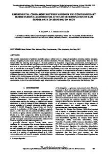
In this section, test runs are described and analyzed for various experiments with different parameter settings. In all test runs, bipartite graphs are denoted as G = (V0, V1, E). Population size should be large enough in order to give an unbiased view of the search space. On the other hand, too large population size makes the algorithm computationally intractable. Mutation rate increases the variability of the population. Naturally, there is again in a tradeoff situation: if a mutation rate becomes too large (i.e. close to 1.0), the algorithm wanders aimlessly in the search space. On the other hand, mutation rate should not be too low, since no crossover operations are used in this research. Number of iterations is also recorded to find out the best result. The maximum number of iterations is 500, which specifies the point where the algorithm stops. Graph density is also used to test the performance of EA. Subsequently, BC heuristic is also compared against the EA. All test results represent the averages of multiples runs of the EA on the same graph. As a measure of the dispersion of the results, standard deviation is calculated in various scenarios. When graph size is 10 and the graph density ranges from 10 to 90%, the number of crossings for the BC and EA is always the same for all test runs, whereas the number of iterations needed by EA to outperform the BC is different from one run to another. The mutation rate for the EA was set to 0.8. In this analysis various sets of data have been considered. Fig. 4 shows the performance of the evolutionary model compared with the BC heuristic approach, where graph order set to 10 and graph density equal to or less than 90%. In this figure, the population size for the EA is set to 10. Having a relatively small population size, the number of iterations needed to outperform the BC heuristic reached 200.

Number of Crossings (BC) Number of Crossings (EA) 35 30 25 20 15

10 5 0 0.2

0.3

0.4

0.5

0.6

0.7

0.8

0.9

Graph Density

Fig. 5: BC Heuristic vs. EA (Pop. Size = 30) In terms of performance, Fig. 5 shows quite similar results as Fig. 4 except that the EA population size parameter is changed to 30. With a more diverse population, the EA needed less number of iterations to outperform the BC heuristic. The number of iterations to find less number of edge crossings did not exceed 50. As the graph order increases, small population size such as 10 would need as much as 500 iterations to get the same results. When population size is increased to 50 or 70, the number of iterations has slightly increased. Population sizes used in Fig. 6 and 7 were 30 and higher for any graph order equal 17. Fig.6 shows that the EA always outperforms the BC heuristic for graphs with densities greater than 50%. Figure 7 also illustrates the performance of the EA compared to the BC heuristic on graphs of order 17 and densities less than 50%. As the graph order increases, the number of edge crossings will always be smaller compared to graphs with small densities as it is indicated in Fig. 6 and 7. Finally, Fig. 8 shows how the graph density affects the number of iterations needed for EA to outperform the BC heuristics. 720

J. Computer Sci., 3 (9): 717-722, 2007 Number of crossings (BC) 100 90 80

They also studied other factors, besides minimizing edge-crossing, that are used when drawing graphs. A simple method was shown for acquiring and satisfying the subjective preferences of the users in order to good layouts. In this study, experiments were conducted to show the performance of EA compared to the BC heuristic. Results indicate that for small graphs or relatively larger graphs, EA always found less number of crossings needed than in the BC heuristic approach. In small graphs for example, where the graph order was set to 10, the graph density did not make any differences as far as the performance of both approaches was concerned. However, when graph order was set to 17, the density factor was important, i.e., higher density graphs generated more edge crossings than lower density graphs. The effectiveness of evolutionary computations depends on the interaction of representations used for the problem solutions, the reproduction/selection operators used and the configuration of the EA used. This research has demonstrated the power that exists within the evolutionary model, which outperforms the traditional methods, especially when the EA parameters are well tuned.

Population size (EA) Number of crossings (EA)

70 60 50 40 30 20 10 0 0.6 0.6 0.6 0.6 0.7 0.7 0.7 0.7 0.8 0.8 0.8 0.8 0.9 0.9 0.9

Graph density

Fig. 6: BC heuristic vs. EA for graphs of densities greater than 50% Number of crossings (BC) Population size (EA) 100 80

Number of crossings (EA)

60 40 20 0 0.1

0.1

0.2

0.2

0.3 0.3 Graph density

0.4

0.4

0.4

Fig. 7: BC Heuristic vs. EA for graphs of densities less than 50% 250

1.

Number of Iterations (EA)

200 150 100 50 0

REFERENCES

Density percent

1

3

5

7

9

11 13

15

17 19 21

2.

23

Averaged test

3.

Fig. 8: Graph density vs. number of iterations CONCLUSION

4.

[16]

studied minimizing edgeRosete-Suarez et al. crossing with an evolutionary graph drawing and found interesting results. They found that scarce graphs with almost the same number of nodes (20 or 30) as the dense graphs are much easier for the algorithm than dense graphs, which indicated that the number of nodes was not a good indication of the problem difficulty. Consequently, another comparison was made with regards to the number of edges for dense graphs with 20 nodes and around 48 edges and they concluded that a closer relation was found between problem difficulty and the number of edges than the number of nodes.

5. 6.

7.

721

Jing, Y. and K. Cheng, 2001. Vector generation for power supply noise estimation and verification of deep submicron designs. IEEE Transactions on Very Large Scale Integration (VLSI) Systems, 9 (2): 329-340. Merz, P. and F. Bernd, 2000. Fitness landscapes, mimetic algorithms and greedy operators for graph bipartitioning. Evol. Comp., 8 (1): 61-91. Garey, M.R. and D.S. Johnson, 1983. Crossing Number is NP-Complete. SIAM J. Algebraic and Discrete Methods, 4 (3): 312-316. Jünger, M. and P. Mutzel, 1997. 2-Layer straightline crossing minimization: Performance of exact and heuristic algorithms. J. Graph Algorithms Appl., 1: 1-25. Marti, R., 1998. Tabu search algorithm for the bipartite drawing problem. Eur. J. Operat. Res., 106 (2-3): 558-569. Stallmann, M., F. Brglez and D. Ghosh, 2001. Heuristics, Experimental Subjects and Treatment Evaluation in Bigraph Crossing Minimization, ACM J. Exp. Algorithmics, 6: (8): 1-42. May, M. and K. Szkatula, 1988. On the Bipartite Crossing Number. Control CyberNet, 17 (1): 85-98.

J. Computer Sci., 3 (9): 717-722, 2007 8.

9. 10.

11. 12.

13. 14.

15. Newton, M., O. Sykora, M. Withall and I. Vrto, 2002. A PVM Computation of Bipartite Graph Drawings. http://parc.lboro.ac.uk/research/projects/parseqgd/s topara/stopara.pdf accessed on 6th August 2006. 16. Rosete-Suarez, A., M. Sebag and A. OchoaRodriguez, 1999. A study of Evolutionary Graph Drawing. Technical Report, http://citeseer.ist.psu.edu/411217.html accessed on 7th November 2006. 17. Branke, J., F. Bucher and H. Schmeck, 1997. A Genetic Algorithm for Undirected Graphs. In J. T. Alnader Edn., Proceedings of 3rd Nordic Workshop on Genetic Algorithms and their Appli., 193-206. 18. Eades, P. and N. Wormald, 1994. Edge Crossings in Drawings of Bipartite Graphs. Algorithmica, 1: 379-403. 19. Yamaguchi, A. and H. Toh, 2001. Two-Layered Genetic Network Drawings with Minimum Edge Crossings, Genome Informatics, 12: 456-457. 20. Leighton, F.T. and S. Rao, 1988. An Approximate max flow min cut theorem for multicommodity flow problem with applications to approximation algorithm. In the 29th Annual IEEE Symposium on Foundation of Computer Science, IEEE Computer Society Press, Los Alamitos, 422-431. 21. Shahrokhi, F., F. Sykora, L.A. Szekely and I. Vrto, 2001. On Bipartite Drawings and the Linear Arrangement Problem, SIAM J. Comp., 30 (6): 1773-1789.

Lee, K.C., N. Funabiki and Y. Takifuji, 1992. A Parallel Improvement Algorithm for the Bipartite Subgraph Problem. IEEE Trans. Neural Networks, 3: 139-145. Ezziane, Z., 2002. Job Sequencing in an Evolutionary Paradigm. Cybernetics and Systems: An Int. J., 33 (2): 161-170. Ezziane, Z., 2002. Solving the 0/1 Knapsack Problem using an Adaptive Genetic Algorithm. Artificial Intelligence for Engineering Design, Analysis and Manufacturing (AIEDAM), 16 (1): 23-30. Makinnen, E. and M. Sieranta, 1994. Genetic Algorithms for Drawing Bipartite Graphs. Int. J. Comp. Math., 53: 157-166. Kannan, R., P. Tetali and S. Vempala, 1997. Simple Markov-chain algorithms for generating bipartite graphs and tournaments. Proceedings of the eighth annual ACM-SIAM symposium on Discrete algorithms, New Orleans, Louisiana, USA, 193-200. Michalewicz, Z., 1996. Genetic Algorithms+Data Structures = Evolution Programs, 3rd Edn., Springer, New York. Hobbs, M.H.W. and P.J. Rodgers, 1998. Representing Space: A Hybrid Genetic Algorithm for Aesthetic Graph Layout. In Frontiers in Evolutionary Algorithms, FEA’98, Proceedings of the 4th Joint Conference on Information Sciences, JCIS’98, 2: 415-418.

722