Experimental demonstration of gray-scale sparse modulation codes in ...

Experimental demonstration of gray-scale sparse modulation codes in volume holographic storage Brian M. King, Geoffrey W. Burr, and Mark A. Neifeld

We discuss experimental results of a versatile nonbinary modulation and channel code appropriate for two-dimensional page-oriented holographic memories. An enumerative permutation code is used to provide a modulation code that permits a simple maximum-likelihood detection scheme. Experimental results from the IBM Demon testbed are used to characterize the performance and feasibility of the proposed modulation and channel codes. A reverse coding technique is introduced to combat the effects of error propagation on the modulation-code performance. We find experimentally that level-3 pixels achieve the best practical results, offering an 11–35% improvement in capacity and a 12% increase in readout rate as compared with local binary thresholding techniques. © 2003 Optical Society of America OCIS codes: 210.2860, 090.7330.

1. Introduction

Volume holographic memories 共VHM兲 have long been a candidate for next-generation digital storage solutions.1 VHMs offer the potential to provide large storage capacities as well as high aggregate transfer rates. The capacity derives from the ability to multiplex many holographic pages within the same volume element. The transfer rate is achieved by reading and writing data in a massively parallel fashion. Data is stored as a two-dimensional page composed by a spatial light modulator 共SLM兲 containing on the order of one million electronically addressable pixels. The page is retrieved by using a camera of the same resolution 共i.e., pixel matched to兲 the SLM to optically detect the page. The parallelism enables, for example, a millisecond page retrieval rate to produce a gigabit of data per second. The question of how to format binary digital data for storage and subsequent retrieval in a twodimensional optical page has been addressed by a number of researchers. Techniques investigated G. W. Burr is with IBM Almaden Research Center, 650 Harry Road, San Jose, California 95120. M. A. Neifeld is with the Electronics and Computer Engineering Department, University of Arizona, Tucson, Arizona 85721. B. M. King is currently with the Electrical and Computer Engineering Department, Worcester Polytechnic Institute, Worcester, Massachusetts 01609. Received 28 July 2002; revised manuscript received 24 January 2003. 0003-6935兾03兾142546-14$15.00兾0 © 2003 Optical Society of America 2546

APPLIED OPTICS 兾 Vol. 42, No. 14 兾 10 May 2003

cover a broad range of topics including partialresponse signaling,2 tailored channel codes,3,4 decision feedback equalization,5 modulation codes,6,7 smart detector arrays,8,9 low-pass filtering codes,10 and three-dimensional error-correction codes.11 In this paper we theoretically and experimentally investigate the potential system improvements when nonbinary modulation codes are used to format binary data into blocks of gray-scale pixels upon each two-dimensional optical page. More specifically, we focus on a class of sparse permutation modulation codes12 that admit a simple maximum-likelihood decoding solution,13 while simultaneously reducing the optical diffraction efficiency required per page by using fewer bright pixels 共sparse encoding兲. Subsection 2.A introduces the reader to the concept of sparse data pages and elaborates on the relationship between sparsity and holographic diffraction efficiency. In Subsection 2.B we extend the conventionally defined system metric M兾#14 to include grayscale pixels, where each gray-scale pixel level may occur with an arbitrary probability. The relation between M兾# and this sparsity causes the capacity of a VHM to be maximized when data pages contain a larger fraction of darker pixel levels, reducing the overall retrieved power per page. Among the novel contributions of this work is the extension of the sparsity capacity advantage to nonbinary 共gray scale兲 data pages. In Section 3 we discuss experimental results of applying sparse gray-scale codes in the IBM DEMON1 holographic platform.1,7 A variety of code pa-

rameters are evaluated and an upper-bound on system capacity for using such codes is presented. It is found that error propagation upon decoding the modulation code substantially limits the performance of the system. To address this issue a reverse coding scheme15 is introduced in Section 4, and simulation results are presented. It is shown that the errorpropagation problem can be overcome by introducing short block length Reed–Solomon codes in a reverse code concatenation scheme. We conclude with a summary of the expected increase in holographic memory capacity for the best subset of sparse gray-scale codes. 2. Modulation-Encoded Sparse Gray-Scale Holographic Pages A.

Sparse Binary Pages

The experimental results in this paper are based on the improvement in storage capacity offered when VHM pages are modulation-encoded to contain a sparse distribution of gray-scale pixels. In this section we briefly outline the properties of such pages. On average, a conventional holographic-data page contains an equal number of OFF and ON pixels. If there are N pixels in this binary-data page, then the page may represent up to, but not more than N bits of information. Exactly N bits could be encoded if the system noises 共blur, aberrations, fixed imaging distortions, thermal noise, etc. . . . 兲 were not severe enough to degrade the detection of the binary pixels. From this point of view, the system capacity is maximized by simply increasing N until these noise sources limit reliable retrieval of the page. In general, however, all holographic storage materials 共including both photorefractives and photopolymers兲 follow the same relationship between the page-wise diffraction efficiency, ␩p, and the number of pages, M, multiplexed in the same volume of material. The system-metric M兾#14,16 was invented to precisely characterize this relationship: ␩p ⫽

冉 冊

2

M兾# . M

(1)

When ON and OFF pixels in a data page occur with unequal probabilities, then the page diffraction efficiency can be rewritten12 as

冉 冊

M兾# ␩p ⫽ M

2

1 , 2␲ 1

(2)

where ␲1 is the probability of a pixel being in the ON state. By decreasing ␲1 the diffraction efficiency per page can be increased because there are fewer ON pixels sharing the material’s dynamic range. If a minimum diffraction efficiency is required to reliably detect a page, then decreasing ␲1 allows more pages to be stored at the same diffraction efficiency. However, adjusting ␲1 away from 1兾2 also decreases the information content per page. Thus changing ␲1

away from 1兾2 trades off storage of more pages against less information per page. A value of ␲1 ⫽ 1兾4 maximizes the memory capacity 共14% improvement over ␲1 ⫽ 1兾2兲 at the expense of a 20% reduction in the user data rate. References 12 and 17 provide a more detailed theoretical and experimental discussion of this trade-off for binary-data pages. B.

Gray-Scale Pages

The use of nonbinary-data pages for holographic storage, while discussed by several authors,3,18 has not been widespread because of the lack of suitable multilevel SLMs. However, high pixel count gray-scale data pages can be holographically recorded with a binary SLM by using the predistortion technique,19,20 in which the recording exposure of each pixel is individually controlled. This technique was used to experimentally compare the storage of data pages with three through six discrete levels against binaryencoded pages. The presence of both deterministic and random noise sources caused 3-level– data pages to achieve the largest practical user capacity gain of 30%. However, in these experiments each grayscale level occurred with equal probability, and the pixel levels were equally spaced 共i.e., the level-2 pixel was twice as bright as the level-1 pixel兲. It was previously shown17 that for a sparse memory the pixel diffraction efficiency, ␩, associated with a single ON pixel in the page could be expressed as

冉 冊

M兾# ␩⫽ M

2

1 , ␲1 N

(3)

where N is the number of pixels in the data page. We wish to extend that result to establish the relation between pixel diffraction efficiency and the number of stored pages for a sparse memory with L-ary valued pixels. Both the spacings between these L levels, as well as their probabilities of occurrence across the page, will be allowed to vary arbitrarily to maximize storage capacity. It is important to consider arbitrary level spacings because in the experimental results to follow, finite contrast of the SLM will give the OFF pixel a non-zero diffraction efficiency. For each gray-scale pixel level i we wish to find a relation analogous to Eq. 共3兲, determining the proportionality constant, M兾#共i兲, between its pixel diffraction efficiency, ␩i , and the number of pages in the memory, M, such that: ␩i ⫽

冉 冊

M兾# 共i兲 . M 2

(4)

We derive this gray-scale M兾# for photorefractive materials by noting that M兾# is proportional to the modulation depth of the interference pattern between the gray-scale pixel and the reference beam. Expressing the modulation depth as a product of the recording slope and the erasure time constant enables us to take into account the differences due to the gray-scale value of the pixel. 10 May 2003 兾 Vol. 42, No. 14 兾 APPLIED OPTICS

2547

Let the gray-scale pixel level i be indexed from i ⫽ 0 共the darkest value兲 to i ⫽ L ⫺ 1 共the brightest value兲. Also, let the total power in the object beam be Po, and the total power in the reference beam be Pr. The bulk beam ratio is defined as BR ⫽ P r兾P o.

L⫺1

兺P

共i兲

Ni ,

(6)

i⫽0

where Ni is the number of pixels at level i. To conveniently characterize the choice of the relative pixel intensity levels, we define the ratio between the power in each pixel level and the brightest pixel level as A i – P 共i兲兾P 共L⫺1兲.

(7)

The recording slope is proportional to the amplitude of the interference pattern, which for level i pixels is 公Pr P共i兲. The erasure time constant is unaffected by the choice of Ai so long as the total illuminating power, Pr ⫹ Po, remains constant. The M兾# for gray-level i is computed as M兾# 共i兲 ⫽

⫽

⫽

⫽

冑Pr P共i兲

(8)

Pr ⫹ Po

冑Pr

冑P共L⫺1兲Ai 冑Po共BR ⫹ 1兲 冑Po 冑BR BR ⫹ 1

冑BR BR ⫹ 1

⫽ M兾#

冑

冑

(10)

L⫺1

P

兺AN j

j

j⫽0

冑Ai

冑

N

(9)

冑P共L⫺1兲Ai 共L⫺1兲

(11)

L⫺1

N

兺A␲ j

j

j⫽0

冑Ai L⫺1

兺

.

(12)

Aj ␲j

j⫽0

The important result of the above sequence of equations is that the gray-level i-pixel diffraction efficiency can be expressed in terms of the standard system-level definition of M兾# 关defined in Eq. 共1兲兴 if we just include the normalization factor associated with the relative power in each gray-level pixel. The overall relationship between level-i pixel diffraction 2548

␩i ⫽

冉 冊 M兾# M

2

Ai

APPLIED OPTICS 兾 Vol. 42, No. 14 兾 10 May 2003

.

L⫺1

兺

N

(13)

Aj ␲j

j⫽0

(5)

We can express the total object beam power as a sum of the beam power associated with all the pixels at each level. Let the power in each level i pixel be P共i兲 such that: Po ⫽

efficiency and the other VHM system parameters is thus

As a sanity check, notice that for the case of binary equal-probable data with infinite contrast ratio that Eq. 共13兲 simplifies to the definition given in Eq. 共3兲 by using the values: L ⫽ 2, A0 ⫽ 0, A1 ⫽ 1, ␲0 ⫽ 1兾2, ␲1 ⫽ 1兾2. Equation 共13兲 enables us to quantify the capacity of the memory in the presence of the noise sources encountered in the system. In general there will always be a minimum diffraction efficiency required for the system to operate at the desired bit error rate 共BER兲. It is important to note that BER is a monotonic function of the pixel diffraction efficiency. As the diffraction efficiency increases, BER decreases and vice versa. Because the diffraction efficiency for each gray level scales proportionately, we only need to consider the behavior of one gray level. For convenience, we examine the diffraction efficiency of the brightest pixel level, ␩L⫺1. In the experimental results to follow, we measure the mean value of the L ⫺ 1-valued pixels and are able to determine the minimum value of ␩L⫺1 necessary to achieve the BER target. Equation 共13兲 can be rearranged to now establish the maximum number of storable pages for the given system parameters: M⫽

M兾#

1

冑N 冑␩L⫺1

1

冑兺

.

L⫺1

(14)

Aj ␲j

j⫽0

Evaluating Eq. 共14兲 by using the minimum acceptable diffraction efficiency, ␩L⫺1, that corresponds to the maximum acceptable raw BER, BER*, yields the maximum number of storable pages, M*. We will use this result in the experimental section to estimate the system capacity. One further simplification is possible by keeping the laser power and detector conditions 共quantum efficiency, integration time兲 the same for all experiments. We can use the measured pixel counts directly as a replacement for the diffraction efficiency. Because the relationship between measured pixel values and diffraction efficiency remains fixed owing to the fixed power and detection conditions, we can substitute the measured mean camera value of the brightest gray-scale level, ␮L⫺1, for its associated diffraction efficiency, ␩L⫺1. Making these changes to Eq. 共14兲 and considering the case when the maximum acceptable BER requirement 共BER*兲 is met produces M* ⫽

M兾#

1

冑N 冑␮L⫺1*

1

冑兺

L⫺1 j⫽0

Aj ␲j

.

(15)

There is a final detail depending on the specifics of whether gray-scale pixels are achieved by using a time-dynamic binary SLM 共the predistortion method: see Ref. 20兲, or if a gray-scale SLM is used. The differences may change the exposure power ratios 共 A0, A1, . . . , AL⫺1兲 but appropriate compensation will allow any desired set of relative diffraction efficiencies. The previous analysis assumed a grayscale SLM for simplicity. C.

Sparse Nonbinary Modulation Codes

To take advantage of the proposed sparsity gains, an efficient encoding and decoding method is necessary. One such method is based upon an enumerative mapping between sequential binary labels and an ordered list of the sparse code words. The interested reader is directed to Refs. 12 and 13 for a thorough description and analysis of the technical details. These codes are categorized as sparse-nonbinarymodulation codes. With respect to this paper, it is sufficient to consider the sparse code as encoding a block of random binary user data into a L-ary–valued data block. The output block always has the same distribution of gray-scale pixel values 共␲j is the same for every block兲. To decode the gray-scale code word, a simple sort-based maximum-likelihood algorithm exists that outputs the estimate of the binary user data. The code is parameterized by the block length 共n兲, the number of gray levels 共L兲, and the number of pixels at each gray level 共兵n␲0, . . . , n␲L⫺1其兲. 3. Experimental Results

On the IBM DEMON1 platform, we recorded and recovered pages encoded using a variety of sparse binary and nonbinary modulation codes. The set of experiments demonstrate the trade-off between code rate, block length, and the estimated capacity gain 共or loss兲. Tables 1 and 2 describe the codes under test and their associated parameters. Block lengths of 9, 12, 24, 48, 64, and 90 pixels were used to cover the practical range of values. Clearly, small block lengths such as 9 pixels have a low code rate and hence are not expected to offer a systematic improvement. Similarly, a block length of 90 pixels may not be advantageous. Such longer blocks suffer a sharp BER performance loss due to the effect of error propagation: even a single pixel error can lead to a large number of bit errors within the decoded code word. A block length somewhere between these two extremes is expected to provide the best practical capacity improvement. The upper bound on the code rate 共RE兲 is established by the entropy of a random source producing the desired pixel distribution statistics. The “% Entropy” column of Table 2 computes the percentage of entropy each modulation code achieves, e.g., how efficiently each encoding scheme achieves the particular set of ␲j values. It has been discussed previously that by using nonbinary valued pixels will improve the system capacity. It was inferred in Ref. 19 that due to practical system issues 3-ary valued pixels are the best choice.

Table 1. Experimental Data Sets and Key Parameters of Interest 共Part I兲

# Pixels per Gray Level

Set

User Bits k

Block Length n

m0

m1

m2

m3

Rate RE

A21 A22 A23 A24 A25 A26

5 7 17 36 48 68

9 12 24 48 64 90

7 9 18 36 48 68

2 3 6 12 16 22

— — — — — —

— — — — — —

0.555556 0.583333 0.708333 0.75 0.75 0.755556

A31 A32 A33 A34 A35 A36

7 10 24 54 72 104

9 12 24 48 64 90

6 8 16 31 42 59

2 3 6 12 16 22

1 1 2 5 6 9

— — — — — —

0.777778 0.833333 1 1.125 1.125 1.15556

A42 A43 A44 A45 A46

13 30 63 88 124

12 24 48 64 90

7 14 29 38 54

3 6 12 16 23

1 3 5 7 9

1 1 2 3 4

1.08333 1.25 1.3125 1.375 1.37778

B31 B32 B33 B34 B35 B36

8 11 27 59 80 115

9 12 24 48 64 90

5 7 14 28 37 52

3 4 7 14 19 27

1 1 3 6 8 11

— — — — — —

0.88889 0.916667 1.125 1.22917 1.25 1.27778

B41 B42 B43 B44 B45 B46

10 15 33 71 97 140

9 12 24 48 64 90

5 6 13 25 34 48

2 3 6 13 17 23

1 2 3 7 8 12

1 1 2 3 5 7

1.11111 1.25 1.375 1.47917 1.51562 1.55556

In this experiment we compare codes using binary, 3-ary, and 4-ary valued pixels. As summarized in the results section, we concur with the previous finding that 3-ary valued pixels offer the best experimental capacity. We begin by describing the code parameters and the testing procedure followed in the experiment. In Subsection 3.B we discuss how to compute the extrapolated system capacity based on the measurements from the experimental data. A local threshold detection scheme by using knowledge of the true data is introduced in Subsection 3.C to provide a baseline comparison of the various proposed modulation and detection schemes. In Subsection 3.D we compute, plot, and discuss the results of the experiment. A.

Testing Procedure

The goal of these experiments was to characterize the retrieval BER performance of the proposed coding techniques, as well as the reference case of no coding. To achieve these results, we implemented the following experimental procedure for each set of code parameters under test. 10 May 2003 兾 Vol. 42, No. 14 兾 APPLIED OPTICS

2549

Table 2. Experimental Data Sets and Key Parameters of Interest 共Part II兲

Set

Block Length n

␲0

␲1

␲2

␲3

% Entropy

A21 A22 A23 A24 A25 A26

9 12 24 48 64 90

0.778 0.750 0.750 0.750 0.750 0.755

0.222 0.250 0.250 0.250 0.250 0.245

— — — — — —

— — — — — —

72.7 71.9 87.3 92.4 92.4 94.2

A31 A32 A33 A34 A35 A36

9 12 24 48 64 90

0.667 0.668 0.667 0.646 0.656 0.656

0.222 0.250 0.250 0.250 0.250 0.244

0.111 0.082 0.083 0.104 0.094 0.100

— — — — — —

63.5 70.1 84.1 90.2 92.3 94.1

A42 A43 A44 A45 A46

12 24 48 64 90

0.582 0.583 0.604 0.594 0.600

0.250 0.250 0.250 0.250 0.256

0.084 0.125 0.104 0.109 0.100

0.084 0.042 0.042 0.047 0.044

69.8 82.3 89.3 91.5 93.3

B31 B32 B33 B34 B35 B36

9 12 24 48 64 90

0.556 0.583 0.583 0.583 0.578 0.578

0.333 0.333 0.292 0.292 0.300 0.300

0.111 0.083 0.125 0.125 0.125 0.122

— — — — — —

65.8 71.6 83.5 91.2 92.4 94.7

B41 B42 B43 B44 B45 B46

9 12 24 48 64 90

0.556 0.500 0.542 0.521 0.531 0.533

0.222 0.250 0.250 0.271 0.266 0.256

0.112 0.167 0.125 0.146 0.125 0.133

— 0.083 0.083 0.062 0.078 0.078

67.0 72.3 81.3 89.3 91.6 93.7

Pixel Priors

1. Thermally erase the crystal. 2. Repeat three times: 共a兲 Move the reference beam to an unused angle 共b兲 Record the hologram by using the predistortion technique20

Fig. 2. Histogram of a 3-level hologram.

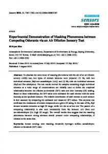
共c兲 Capture the hologram reconstruction over a range of CCD integration times 共typically approximately 19 exposures兲. An example SLM image and corresponding CCD image of the reconstructed hologram are shown in Fig. 1. The histogram of the hologram is presented in Fig. 2. The crystal was not always erased between sets. On average, it was erased after every four data sets were acquired. For each hologram we retrieved approximately 19 images using a variety of exposure times. These images are decoded to provide an estimate of both the pixel-error rate 共PER兲 and the decoded user BER. In addition to decoded error rates, we compute the mean and variance of each of the L-pixel levels, which we refer to as ␮i and ␴i 2, respectively, for i 僆 兵0, 1, . . . , L ⫺ 1其. The PER is estimated by counting the errors incurred by thresholding the pixel data by use of the best possible threshold 共i.e., the threshold that minimizes the PER兲. The user BER is estimated by decoding the

Fig. 1. 共a兲 Example of an SLM image, 共b兲 reconstructed hologram for a 3-ary valued pixel case. 2550

APPLIED OPTICS 兾 Vol. 42, No. 14 兾 10 May 2003

Fig. 3. Experimental data and curve fit of gray-scale level 2 mean pixel value to bit-error-rate for the XA32 data set.

data and counting the percentage of data bits in error. We plot BER against ␮L⫺1 to determine the minimum required pixel mean, ␮L⫺1*, which achieves the desired bit error rate, BER*. Figure 3 shows an example curve from the A32 code. From the graph we see that for the XA32 set, ␮2* ⫽ 26.4 for BER* ⫽ 10⫺3. This procedure can be repeated for each code. B.

Estimated Capacity

From the BER versus the pixel mean experimental curve fits, we use Eq. 共15兲 to estimate the number of pages in the VHM and hence the capacity provided by each set of codes and associated parameters. It should be noted that the capacity refers to a single addressable volume element of the storage medium. In a practical VHM, there may be thousands of such elements within the storage medium. This capacity estimate assumes the diffraction efficiency scales as 1兾M 2 and that the storage of the additional pages in the memory does not degrade the fidelity of the already stored holograms; only the diffraction efficiency of the holograms is reduced. We know from earlier work21 that this assumption is somewhat optimistic, because the consecutive storage of the data pages does affect the hologram fidelity to some degree. However, the capacity estimates obtained by this approach provide an upper bound on the practical storage capacity. With that caveat in mind, we convert our experimental data to a capacity estimate by the following procedure: 1. Curve fit the decoded user BER versus the mean of the brightest gray-level pixels, ␮L⫺1

2. Find ␮L⫺1* that achieves the target raw BER, BER*. 3. Compute the estimated number of stored pages by using the analysis developed in Section 1. 4. Compute the estimated capacity as C ⫽ M*NR,

(16)

where R is the overall system code rate due to modulation and error correction coding, or equivalently, the number of user bits represented per pixel. To develop a better understanding of the many factors affecting the capacity estimate, C, we can reexpress Eq. 16 in terms of five factors: C ⫽ M*NR

(17)

⫽ 共F M兲关F B兴共S兲 R E R 0 ⫽ 共M兾# 冑2N兲

(18)

冤 冑 冥冢 冑 兺 冣 1

␮ L⫺1*

1

L⫺1

R E R 0.

(19)

Aj ␲j

2

j⫽0

Here FM is the holographic-system factor that describes the effects of M兾# and the number of pixels per page. Note that this factor also carries an implicit factor describing the efficiency with which diffracted photons are converted to camera counts 共e.g., laser readout power, camera integration time quantum efficiency, and background electronic noise兲. However, for the purposes of comparing different codes measured under otherwise identical conditions, this factor can be ignored. FB indicates the relative diffraction efficiency that is required to satisfy the 10 May 2003 兾 Vol. 42, No. 14 兾 APPLIED OPTICS

2551

BER specification with a given code, S describes the gain realized by that code due to the combination of sparseness and multiple pixel levels, and RE is the code rate of the shortened enumerative permutation code 共the efficiency with which the sparseness and multiple pixel levels are encoded兲. R0 is then the code rate of any remaining error-correction or modulation coding that corrects the target decoded raw BER, BER*, down to an acceptable user BER on the order of 10⫺12. The extra factor 公2 in the denominator of S 共which is balanced by the inclusion of a similar factor in the numerator of FM兲 normalizes the sparsity gain to unity for the case of random binary data. However, for more than two gray levels, the actual achieved sparsity gain S may be less than ideal, simply because the actual spacings between the levels may differ when the holograms are recorded. In fact, because the noise variances of each pixel level vary 共tending to broader distributions for higher levels兲, altering the spacings of the pixel levels can also reduce the BER, at a cost in sparsity gain. We keep track of this difference by considering both S, the actual sparsity gain using the level spacings implemented in our experiments, as well as SI, the ideal sparsity gain that would be achieved with equally spaced pixel levels. We define ␥ such that S ⫽ ␥SI, where ␥ must be in the range 关0,1兴. Because the ideally spaced levels for L-ary valued pixels are Bj –

j⫺1 , L⫺1

(20)

which differ from Aj , the set of levels actually implemented in experiment. We can thus compute ␥ directly as

冑 兺 冒兺 L⫺1

␥⫽

Aj ␲j .

(21)

j⫽0

Thus for any sparse code, SI is greater than unity, directly representing the factor by which sparseness and multiple pixel levels increase the storage capacity over the uncoded binary case. If this code is successful, then this sparsity gain will outweigh the penalties for using this code from FB and RE, e.g., a successful code delivers high sparsity gain while still decoding weak holograms to the target BER* with high coding efficiency. Local Threshold Detection

To provide a baseline comparison with the enumerative permutation code results, we also employ a local threshold-detection scheme for the binary pixel data sets. This detection method works by processing the page in 8 ⫻ 8 pixel blocks and by computing the histogram of the 64 pixels. From that histogram and the true knowledge of the transmitted-data page we exhaustively find the threshold that minimizes the BER of the block. This is an upper bound on the performance of a local thresholding scheme because it uses the 共necessarily unavailable in practice兲 true 2552

Sparsity Factor ␥

BER Factor FB

1

0.9600

0.2441

1

2510 2143 2215 2018 2043 2046

1.500 1.414 1.414 1.414 1.414 1.430

0.9352 0.8997 0.9297 0.9223 0.9369 0.9353

0.2902 0.2732 0.2733 0.2510 0.2502 0.2481

0.5556 0.5055 0.7083 0.7500 0.7500 0.7556

1.122 1.212 1.358 1.389 1.323 1.084

1665 1677 1567 1425 1357 1082

1.500 1.549 1.549 1.477 1.512 1.500

0.9134 0.9031 0.9008 0.9103 0.9018 0.8979

0.1971 0.1944 0.1822 0.1719 0.1614 0.1303

0.7778 0.8333 1.0000 1.1250 1.1250 1.1560

XA42 XA43 XA44 XA45 XA46

1.107 1.183 1.212 1.169 1.027

1179 1092 1065 981 860

1.500 1.549 1.604 1.569 1.596

0.8881 0.9285 0.9052 0.9123 0.9103

0.1436 0.1231 0.1191 0.1112 0.0961

1.0830 1.2500 1.3120 1.3750 1.3780

XB31 XB32 XB33 XB34 XB35 XB36

1.130 1.194 1.270 1.351 1.268 1.324

1467 1503 1302 1268 1170 1196

1.342 1.414 1.359 1.359 1.352 1.355

0.9280 0.9207 0.9252 0.9184 0.9294 0.9306

0.1911 0.1872 0.1680 0.1649 0.1511 0.1538

0.8889 0.9167 1.1250 1.2290 1.2500 1.2780

XB41 XB42 XB43 XB44 XB45 XB46

1.071 1.044 1.104 1.073 1.033 0.845

1112 964 926 837 786 627

1.389 1.342 1.414 1.414 1.414 1.409

0.9208 0.9297 0.9277 0.9046 0.9021 0.9191

0.1411 0.1254 0.1145 0.1062 0.1000 0.0785

1.1110 1.2500 1.3750 1.4790 1.5160 1.5560

Set

Capacity 关Gbits兴

Pages M*

XC20

1.252

1445

XA21 XA22 XA23 XA24 XA25 XA26

1.208 1.083 1.360 1.312 1.328 1.340

XA31 XA32 XA33 XA34 XA35 XA36

Ideal Sparsity SI

Rate RE

L⫺1

Bj ␲j

j⫽0

C.

Table 3. Experimental Capacity Parameters

APPLIED OPTICS 兾 Vol. 42, No. 14 兾 10 May 2003

data to choose the best-possible local-decision threshold. The conversion of the minimum required pixel value 共using the local threshold兲 to a capacity estimate is identical to that of the enumeration-based codes. In fact, we consider the local threshold as a sort of code that has a code rate, RE, of unity 共1 bit per pixel兲, and a sparsity factor of unity. D.

Results

The results of the various codes are summarized in Table 3. Set XC20 is local threshold detection, and the other codes have all been previously defined in Tables 1 and 2. Fig. 4 shows the results with the capacity plotted against the number of pages in the memory for the XC20, XA2, XA3, XA4, XB3, and XB4 sets. For these results, BER* ⫽ 10⫺3. To achieve an output user BER of ⬍10⫺12, an outer Reed–Solomon 共RS兲 code is applied with a code rate of R0 ⫽ 0.8667. The outer RS共255, t ⫽ 17兲 code yields an output user BER of 6.2 ⫻ 10⫺13 for the given BER*. Notice that using these modulation codes causes a change in the readout rate of the VHM in addition to the change in capacity. The system M兾# value of

Fig. 4. Experimental estimated VHM capacity. The lines connect symbols that differ only in the code block length parameter 共all other code parameters remain the same兲.

4358.9 taken from Ref. 22 assumes a page readout rate of 1 kHz with 106 pixels per page. So threshold detection operates at an aggregate transfer rate of 1 Gbit兾s. In Table 4, we summarize the relative change in capacity and readout rate achieved for each experimental data set. We see that the best performing code is the A34 code: 48 pixels per code word, 31 “0” pixels, 12 “1” pixels, and 5 “2” pixels. Each pixel represents 1.125 bits of information. This code achieves a 10.93% increase in capacity and a 12.5% improvement in the readout rate as compared with no modulation coding and a local threshold detection scheme. 4. Error Propagation

The results in the previous section showed that sparse nonbinary enumerative permutation codes can improve the VHM capacity. However, the phenomenon of error propagation degraded those results significantly. We initially described error propagation in Section 3, but we briefly review here the fundamental cause. To achieve an efficient enumeration code rate 共approaching entropy兲, long blocks must be used. The nondistance preserving mapping between the input and output of the enumeration code results in a small number of symbol errors present in the code word decoding to a much larger number of bit errors in the output data. The severity of error propagation can be characterized by looking at the magnification in the error rate upon decoding. If error propagation is present, a few errors at the input of the decoder will lead to a large number of errors in the decoded code word. Ideally, this error-rate magnification would

Table 4. Change in Capacity and Readout Ratea

Set

Capacity Change 共%兲

Readout Rate Change 共%兲

XA21 XA22 XA23 XA24 XA25 XA26

⫺3.53 ⫺13.49 8.58 4.77 6.09 6.99

⫺44.44 ⫺41.67 ⫺29.17 ⫺25.00 ⫺25.00 ⫺24.44

XA31 XA32 XA33 XA34 XA35 XA36

⫺10.38 ⫺3.25 8.44 10.93 5.67 6.99

⫺22.22 ⫺16.67 0 12.50 12.50 15.60

XA42 XA43 XA44 XA45 XA46

⫺11.63 ⫺5.54 ⫺3.25 ⫺6.64 ⫺17.99

8.30 25.00 31.20 37.50 37.80

XB31 XB32 XB33 XB34 XB35 XB36

⫺9.76 ⫺4.64 1.38 7.89 1.25 1.25

⫺11.11 ⫺8.33 12.50 22.90 25.00 27.80

XB41 XB42 XB43 XB44 XB45 XB46

⫺14.46 ⫺16.61 ⫺11.83 ⫺14.33 ⫺17.51 ⫺32.50

11.10 25.00 37.50 47.90 51.60 55.60

a Readout rate relative to the case of binary pixels and no modulation coding 共local-threshold detection兲.

10 May 2003 兾 Vol. 42, No. 14 兾 APPLIED OPTICS

2553

Fig. 5. Histogram of the number of bit errors incurred when decoding random codewords from code A46 with weight 2 error patterns.

be a small factor, but with these enumerative permutation codes, it tends to scale with the code block length n. To help understand the magnitude of this effect, consider the following simulation: we take various code words selected from the A46 code 共n ⫽ 90 pixels, L ⫽ 4兲, and corrupt them with a random weight 2 error pattern 共2 random locations are swapped兲. This corresponds to the most likely error event we will encounter upon retrieval of the holographic-data page 共single or odd-weight error patterns are not possible in constant-weight codes兲. The corrupted code word is decoded and the Hamming distance is computed between the actual and decoded 124 user bit sequences. This process is repeated many times, and we form a histogram of the number of user bit errors incurred by a weight 2 code word error. Figure 5 shows the histogram. A nearest-neighbor code word error generates on average approximately 40 bit errors 共30% of the user data block兲. To combat this problem we propose a concatenated coding scheme as suggested in Refs. 15, 23–25. We will refer to the method as reverse coding owing to the reversed application order of an algebraic errorcorrection code 共ECC兲. Typically, user data is encoded with an outer strong ECC followed by a modulation code. We propose adding an inner weaker high-rate ECC after the modulation code to protect the modulation code word from errors. Essentially, if we can correct the code word errors incurred in the channel, then there is no error propagation. When we fail to correct all the errors, the error magnification penalizes the decoder. There are a number of optimizations that can be done to implement the reverse coding scheme. We will only consider a basic approach here. 2554

APPLIED OPTICS 兾 Vol. 42, No. 14 兾 10 May 2003

We begin by expressing the number of gray-scale levels, L, in the form L ⫽ qb, where b is an integer. Hence we can represent a pixel value as a length-b sequence of q-ary symbols. Furthermore, we restrict our attention to only the cases where q is prime. In practice, this is not much of a restriction as it handles the interesting cases of L ⫽ 兵2, 3, 4 ⫽ 22, 5其. For the inner code we choose a systematic RS code defined over the finite field GF共qm兲. It is important to distinguish between the two ways we are grouping the data: as L-ary valued pixels 共for the data page兲, and as sequences of q-ary valued symbols 共for the RS code兲. The parameters of the code words are defined in Table 5. We follow the standard convention of defining the RS code as RS共N, K, t兲, where N is the number of q-ary symbols in each code word, K is the number of symbols of information to be encoded in the block, and t is the symbol error-correction ability of the code. We concatenate a sparse code words together and ˜,K ˜ , t兲. We make a feed them to the RS code: RS共N as large as possible to fit as many code words as ˜ ⫽ 共qm ⫺ 1兲 ⫺ 2t RS symbols. possible into the K However, there will be a small leftover number of unused symbols because n does not divide 关共qm ⫺ 1 ⫺ 2t兲m兾b兴 without a remainder in general. To improve the code performance, the unused symbols are Table 5. Inner-Code Parameters

Parameters

qm-ary Symbols

L-ary Pixels

Input data Parity Length Shortened Length

K 关anb兾m兴 P 2t ˜ qm ⫺ 1 N N K⫹P

an 关2tm兾b兴 关共qm ⫺ 1兲m兾b兴 —

Fig. 6. Block diagram of reverse encoding scheme. 共a兲 Type I: parity pixels violate sparse constraint. 共b兲 Type II: parity pixels meet sparse constraint due to encoding with enumeration code E2.

discarded from the code yielding a shortened RS code: RS共N, K, t兲. Note that shortening the code preserves the maximum distance separation 共MDS兲 property of the original RS code.26 The code word is protected up to t symbol errors, meaning that if there are t or less incorrect symbols in the detected code word, the RS code will always correct them. Encoding is a straightforward procedure as depicted in Fig. 6. The user data protected with a strong outer ECC code is encoded with the modulation code E1 producing a code word, C, that is a concatenation of a enumeration codewords. C is treated as a length K RS information symbol block input to the inner systematic RS code which outputs the 2t symbols of parity. The parity symbols are expressed as pixels and appended to C to produce a new protected code word C⬘ ⫽ 关C兩P兴. Protecting the code word requires an additional 关2tm兾b兴 pixels. We consider two types of reverse codes: type I and type II. In the type I approach 关Fig. 6共a兲兴, the parity from the RS code is encoded directly into pixels that do not satisfy any modulation constraint 共sparse or otherwise兲. Type-II codes 关Fig. 6共b兲兴 encode the RS parity with another enumeration code, E2, to produce a longer sequence of parity pixels that do satisfy the sparse modulation constraint. It is clear that the parity in the type-II code may suffer from error propagation as did our original unencoded code word. We expect t to be small and hence the parity sequence to be significantly shorter than the enumeration code word. In this case, the error propagation incurred on the parity pixels will hopefully be small as well. Another obvious extention of the type-II code, is to repeat the protection and re-modulation coding of the parity recursively on the parity from the previous code stage. For example, a type-III code could be defined by protecting the modulation-constrained parity from the type-II code with a new 共shorter兲 RS code. The new parity is then modulation encoded and appended to the sequence. This would help to combat the error propagation in the parity code word. Clearly this process could be repeated until an imple-

mentational complexity issue is raised. We will only consider the type-I and type-II codes in this paper. A.

Implementation Details

There are a number of minor details that have to be addressed when considering encoding the RS GF共qm兲 symbols in terms of L-ary 共qb兲 pixels. Thoughtful consideration will solve most of these at the expense of a partially utilized 共wasted兲 pixel or two. In general, a block of r RS symbols represents mr q-ary digits of information, which can be expressed as 关rm兾b兴 pixels. The number of pixels wasted 共due to the ceiling function兲 will therefore be at most 1 pixel. Blocking the symbols into pixels in this manner results in a pixel possibly containing information associated with two symbols. The decoding complexity is not sabotaged by this fact because it is a trivial matter 共in hardware or software兲 to treat each raw decoded L-ary pixel as a serial concatenation of b q-ary digits. Data from each pixel is appended to this stream of q-ary digits until m of them have been captured, and the next qm symbol of the RS code can be output. Any remaining digits from the last pixel are shifted to the beginning of the conversion register and the process repeats for the next symbol. However, there is an issue concerning detection on the parity portion of the type-I reverse code. By encoding the parity symbols directly into pixels, we do not meet the sparse modulation constraints imposed by the first enumeration code. This decreases the sparsity capacity advantage by increasing the priors associated with the brighter pixel values. It also prevents us from applying the sort-based maximum likelihood detection algorithm.13 Instead, simulations use a thresholding scheme for these constraintviolating pixels. The detection threshold is placed halfway between each possible gray level. This is clearly not the best approach, but it is a reasonable solution. Some of the more obvious disadvantages include the unequal error rate for the end gray level 共levels: 0 and L ⫺ 1兲 transition probabilities as well as the danger of local intensity variations in the re10 May 2003 兾 Vol. 42, No. 14 兾 APPLIED OPTICS

2555

an increase in the BER in the case of high SNR. This strange trend occurs due to the increased error propagation as the enumeration-encoded parity code word is lengthened. C.

Fig. 7. Unprotected BER performance of the A4 set of codes 共n ⫽ 兵12, 24, 48, 90其, L ⫽ 4兲. Error propagation limits the performance of the long codes.

trieved page requiring a form of adaptive threshold tracking and estimation. B.

Simulation Results

To demonstrate the effect of error propagation, the reader is directed to Fig. 7, which shows the BER performance on the A4 set of codes on a simple nonVHM channel. All five codes have effectively the same prior symbol distribution and only differ in block length. A42 is 12 pixels long, while A46 is 90 pixels long. The loss in performance for longer codes is caused by the onset of error propagation. Figure 8 shows the BER of the A46 enumeration code on the same channel. The five curves range from t ⫽ 0 共no reverse coding兲 to t ⫽ 8. As an indicator to the power of the type-I code, we see that the t ⫽ 8 code offers a signal-to-noise ratio (SNR) improvement of 2 dB at a raw BER of 10⫺3. The cost in achieving the lower operating SNR is the 0.935 code rate. Figure 8共b兲 shows the type-II code performance. Note the unusual trend that increasing the error correction ability beyond t ⫽ 4 actually leads to

Reverse Coding Applied to the Experiment

At this point, we would like to apply these reversecoding techniques to our experimental data. However, these data pages were not encoded with any of the required inner ECC. Thus we must formulate a method to use the existing measured data to predict the expected BER 共and capacity兲 improvements offered by reverse coding. We would like to find a prediction that can be justified as either matching or bounding the performance in a complete experiment with reverse coding. The procedure to apply the reverse coding is as follows. We begin with the target raw BER goal of the modulation code 共typically 10⫺3兲. From simulations based on an additive white Gaussian noise 共AWGN兲 channel, we calculate the SNR necessary to achieve the target BER using the reverse code under test. Evaluating the theoretical BER of the enumeration code without reverse coding at this SNR yields the higher unprotected BER 共UBER兲. Because the experimental data represents the same parameters and algorithm as the uncoded enumeration code, we expect the UBER to be representative of the raw error rate we should observe in the experiment. Following the procedure developed earlier for estimating the capacity change due to the enumeration codes, we curve fit the experimental decoded raw BER versus the mean L ⫺ 1 pixel value and find the mean level that achieves the UBER requirement 共as opposed to the BER* requirement without reverse coding兲. The reduction in the required operating pixel mean level represents the improvement in storage capability due to reverse coding, through the BER factor, FB, from Eq. 19. Of course, the lower mean pixel values are achieved at a reduction in the code rate, reflected in the capacity factor R0. For the type-I codes that do not meet the sparsity constraint, we also recompute

Fig. 8. Reverse coding on the A46 共n ⫽ 90, L ⫽ 4兲 code using an inner RS共255, K, t兲 code. 2556

APPLIED OPTICS 兾 Vol. 42, No. 14 兾 10 May 2003

Fig. 9. Comparison of theoretical and experimental input兾output error-rates for data sets XA2, XA3, XA4, and XB4.

the sparsity factor ␥ to include the adjustment to the prior gray-level probabilities. We expect that for small values of error-correction t, the capacity will be improved until a point is reached where increasing t does not provide enough of an increase in FB to cover the loss in R0 and ␥. To partially justify this capacity extrapolation based on theory and experiment, we must consider the possible large effect of the difference between the true experimental noise and the theoretically assumed thermal noise. Figure 9 plots the raw PER versus the decoded user BER for both the theoretical and experimental results. The strong agreement between the output BER for all input PERs indicates that the theoretical simulations can predict, with high accuracy, the experimental output BER from the raw PER. We will use this relation when estimating the extrapolated capacity of the reverse coding schemes applied to the experimental data sets. For each data set we apply both the type-I and type-II reverse codes with varying levels of error correction 共typically t ⫽ 2 up to t ⫽ 10兲 and compare them with the error propagation dominated case. Figure 10 presents the capacity versus the page count for the various codes. As with the previous graphs, the upper left-hand side corner represents

the best location, providing the highest storage capacity available in the fewest number of pages 共highest data rate兲. Each curve is composed of extrapolated results over the range of experimental block lengths. The curve ends denoting the shortest 共9 –12 pixels兲 and longest 共90 pixels兲 blocks used are marked by the set name. It is clear that much of the capacity lost due to error propagation is recovered by the use of reverse coding. In the case of 3-ary pixels, the capacity rises from 1.4 Gbits to 1.7 Gbits, a 21% increase. However, 4-ary pixels achieve a 13% improvement. It is important to note that without reversing coding, long block lengths resulted in reduced performance due to error propagation. However, with reverse coding the longer block lengths yield an improved performance. This trend is clearly illustrated by the A3 type-I code that offers the best performance at a block length of 90 pixels. Also notice that the type-II codes perform in general worse than the type-I codes. This indicates that sparse-enumeration encoding of the parity loses more capacity due to lower code rate 共more parity pixels per code word兲 and residual error propagation than it gains due to the ML sort detection and the use of sparse priors. 10 May 2003 兾 Vol. 42, No. 14 兾 APPLIED OPTICS

2557

References

Fig. 10. Extrapolated reverse code performance for XA3 data set. Triangle symbols mark the performance without reverse coding. Applying type I 共circle symbols兲 and II 共square symbols兲 reverse codes significantly improves the capacity. The lines connect symbols that differ only in the code block length parameter 共all other code parameters remain the same兲.

5. Conclusions

Experimental results of our proposed channel code indicate an 11% improvement in the experimental capacity by using 3-ary pixels. This improvement is relative to the use of local-threshold detection on binary pages containing on average equal numbers of ON and OFF pixels. Because local-threshold detection uses implicit knowledge of the stored data, it should be interpreted as an upper bound on detection performance when no modulation code is used. Hence the 11% improvement may be larger when compared with realizable threshold detection schemes. If reverse coding is used, the effect of error propagation can be partially mitigated, increasing the estimated capacity improvement to a total of 35%. Note that 4-ary codes achieve a maximum gain of 8%. Theoretical results indicate that the 4-ary codes should outperform the 3-ary codes in the limit of thermal noise dominated detection. However, because of the implicit broadening of the pixel distributions during gray-scale recording, 4-ary valued pixels offer less capacity than 3-ary pixels. This is in agreement with earlier work on nonbinary pixels for use in VHMs.19 In general, sparse enumerative permutation codes can increase the VHM storage capacity, though in practice, because of other important noise sources 共holographic recording fidelity, cross erasure, photovoltaic兲 it may not necessarily be possible to achieve the predicted 50% improvement as suggested in Ref. 13 operating in the thermal noise limit. Error propagation reduces the effectiveness of sparse-enumeration codes, but we find that applying an inner RS code to protect the modulation code word can be used to recover a significant amount of the lost performance at the expense of increased decoder complexity and latency. 2558

APPLIED OPTICS 兾 Vol. 42, No. 14 兾 10 May 2003

1. Holographic Data Storage, H. J. Coufal, D. Psaltis, and G. T. Sincerbox, eds., 共Springer-Verlag, Berlin, 2000兲. 2. B. H. Olson and S. C. Esener, “Partial response precoding for parallel-readout optical memories,” Opt. Lett. 19, 661– 663 共1994兲. 3. J. F. Heanue, M. C. Bashaw, and L. Hesselink, “Channel codes for digital holographic data storage,” J. Opt. Soc. Amer. A 12, 2432–2439 共1995兲. 4. V. Bhagavatula and M. Wong, “Crosstalk-limited signal-tonoise ratio resulting from phase errors in phase-multiplexed volume holographic storage,” in Optical Society of America 1996 Annual Meeting, p. 145 共Optical Society of America, Washington, D.C., 1996兲, session WZ6. 5. J. F. Heanue, K. Gu¨ rkan, and L. Hesselink, “Signal detection for page-access optical memories with intersymbol interference,” Appl. Opt. 35, 2431–2438 共1996兲. 6. A. Vardy, M. Blaum, P. H. Siegel, and G. T. Sincerbox, “Conservative arrays: multidimensional modulation codes for holographic recording,” IEEE Trans. Inf. Theory 42, 227–230 共1996兲. 7. G. W. Burr, J. Ashley, H. Coufal, R. K. Grygier, J. A. Hoffnagle, C. M. Jefferson, and B. Marcus, “Modulation coding for pixelmatched holographic data storage,” Opt. Lett. 22, 639 – 641 共1997兲. 8. M. E. Schaffer and P. A. Mitkas, “Requirements and constraints for the design of smart photodetector arrays for pageoriented optical memories,” IEEE. J. Sel. Top. Quantum Electron. 4, 856 – 865 共1998兲. 9. B. M. King and M. A. Neifeld, “Parallel detection algorithm for page-oriented optical memories,” Appl. Opt. 37, 6275– 6298 共1998兲. 10. J. Ashley and B. Marcus, “Two-dimensional lowpass filtering codes for holographic storage,” IEEE Trans. Commun. 46, 724 –727 共1998兲. 11. T. N. Garrett and P. A. Mitkas, “Three-dimensional error correcting codes for volumetric optical memories,” in Advanced Optical Memories and Interfaces to Computer Storage, P. A. Mitkas and Z. U. Hasan, eds., Proc. SPIE 3468, 116 –124 共1998兲. 12. B. M. King and M. A. Neifeld, “Sparse modulation coding for increased capacity in volume holographic storage,” Appl. Opt. 39, 6681– 6688 共2000兲. 13. B. M. King and M. A. Neifeld, “Low-complexity maximumlikelihood decoding of shortened enumerative permutation codes for holographic storage,” IEEE J. Sel. Areas Commun. 19, 783–790 共2001兲. 14. F. H. Mok, G. W. Burr, and D. Psaltis, “System metric for holographic memory systems,” Opt. Lett. 21, 896 – 898 共1996兲. 15. W. Bliss, “Circuitry for performing error correction calculations on baseband encoded data to eliminate error propagation,” IBM Tech. Discl. Bull. 23, 4633– 4634 共1981兲. 16. G. W. Burr, F. H. Mok, and D. Psaltis, “Angle and space multiplexed holographic storage using the 90° geometry,” Opt. Commun. 117, 49 –55 共1995兲. 17. B. M. King and M. A. Neifeld, “Unequal a-priori probabilities for holographic storage,” in Advanced Optical Data Storage: Materials, Systems, and Interfaces to Computers, P. A. Mitkas, Z. U. Hasan, H. J. Coufal, and G. T. Sincerbox, eds., Proc. SPIE 3802, 40 – 45 共1999兲. 18. Y. Taketomi, J. E. Ford, H. Sasaki, J. Ma, Y. Fainman, and S. H. Lee, “Incremental recording for photorefractive hologram multiplexing,” Opt. Lett. 16, 1774 –1776 共1991兲. 19. G. W. Burr, G. Barking, H. Coufal, J. A. Hoffnagle, C. M. Jefferson, and M. A. Neifeld, “Gray-scale data pages for digital holographic data storage,” Opt. Lett. 23, 1218 –1220 共1998兲. 20. G. W. Burr, H. Coufal, R. K. Grygier, J. A. Hoffnagle, and C. M. Jefferson, “Noise reduction of page-oriented data storage by

inverse filtering during recording,” Opt. Lett. 23, 289 –291 共1998兲. 21. G. W. Burr, W.-C. Chou, M. A. Neifeld, H. Coufal, J. A. Hoffnagle, and C. M. Jefferson, “Experimental evaluation of user capacity in holographic data-storage systems,” Appl. Opt. 37, 5431–5443 共1998兲. 22. M. A. Neifeld and W.-C. Chou, “Information theoretic limits to the capacity of volume holographic optical memory,” Appl. Opt. 36, 514 –517 共1997兲. 23. M. Mansuripur, “Enumerative modulation coding with arbitrary constraints and post-modulation error correction coding

for data storage systems,” in Optical Data Storage 191, J. J. Burke, T. A. Shull, and N. Imamura, eds., Proc. SPIE 1499, 72– 86 共1991兲. 24. K. Immink and A. Janssen, “Error propagation assessment of enumerative coding schemes,” Proc. IEEE International Conference on Communications 2, 961–963 共1998兲. 25. J. L. Fan and A. Calderbank, “A modified concatenated coding scheme, with applications to magnetic data storage,” IEEE Trans. Inf. Theory 44, 1565–1574 共1998兲. 26. S. B. Wicker and V. K. Bhargava, eds., Reed–Solomon Codes and Their Applications 共IEEE Press, New York, 1994兲.

10 May 2003 兾 Vol. 42, No. 14 兾 APPLIED OPTICS

2559