Experimental Demonstration of Multiple Robot Cooperative Target ...

AIAA 2002-4678

AIAA Guidance, Navigation, and Control Conference and Exhibit 5-8 August 2002, Monterey, California

EXPERIMENTAL DEMONSTRATION OF MULTIPLE ROBOT COOPERATIVE TARGET INTERCEPT Timothy W. McLain1∗ 1

Randal W. Beard2

Jed M. Kelsey3

Department of Mechanical Engineering, Brigham Young University, Provo, Utah 84602

2

Department of Electrical and Computer Engineering, Brigham Young University, Provo, Utah 84602

3

Department of Electrical and Computer Engineering, Brigham Young University, Provo, Utah 84602

ABSTRACT This paper presents experimental results for the simultaneous intercept of preassigned targets by a team of mobile robots. The robots are programmed to mimic the dynamic behavior of unmanned air vehicles in constant-altitude flight. In proceeding to their targets, robots must avoid both known static threats and pop-up threats. An overview of the cooperative control strategy followed is given, as well as a description of the robot hardware and software used. Experimental results demonstrating simultaneous intercept of targets by the robot team are presented.

1

INTRODUCTION

Recent military conflicts have demonstrated the strategic value of unmanned air vehicles (UAVs). In the past UAVs have been used primarily for reconnaissance and surveillance purposes. More recently, they have been used in offensive missions as a bombing or missile-launching platform. In these scenarios, UAVs have operated independent of other vehicles with little or no cooperation. Although they have been successful as single agents, UAVs will make greater contributions to military missions as their cooperative capabilities are increased. As cooperative control strategies for teams of multiple UAV agents are developed, the potential impact of UAVs on future military operations will certainly broaden. Cooperative control of multiple-UAV teams is a subject to which increasing attention has been given. Research has focused primarily on three areas: UAV formation flight, cooperative path planning (e.g., rendezvous), and resource allocation (e.g., target assignment). The motivation for formation flight of ∗ Corresponding

author, email: [email protected]

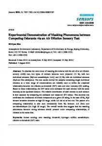
UAVs is increased stealth and fuel economy. In close formations, UAVs are coupled dynamically by the aerodynamic interactions among the vehicles. As such, the entire formation can be considered as a single large system for which a control strategy must be developed. Strategies for formation flight of UAVs are developed in [1, 2, 3, 4]. Unlike formation-flight problems, cooperative path planning and resource allocation problems usually involve UAVs that are physically independent of one another, although they may be coupled dynamically by their cooperative control algorithms. Several important UAV cooperative control problems can be formulated as resource allocation problems. This includes target assignment problems [5, 6], cooperative classification problems [7], and cooperative search problems [8]. The majority of cooperative path planning problems considered in the literature involve timing or sequencing of UAVs for arrival at targets or other specified locations, such as the cooperative intercept problem considered here. A cooperative control strategy for UAV rendezvous was presented in [9]. Cooperative path planning is also employed in cooperative search and cooperative classification problems [10]. Up to the present time, UAV cooperative control research has consisted of simulation studies. This paper presents initial results in cooperative path planning for a team of wheeled robots. These robots are programmed to simulate, in hardware, UAVs in constant-altitude flight. This work presents a decentralized cooperative control strategy and examines its suitability for real-time implementation. The specific problem treated in this paper is similar to that presented in an earlier simulation study [9]. As depicted in Figure 1, three robots must navigate through a field of known threats (depicted by red dots) to arrive at preassigned targets (depicted by stars). The cooperation objective is for

1 American Institute of Aeronautics and Astronautics Copyright © 2002 by the American Institute of Aeronautics and Astronautics, Inc. All rights reserved.

the robots to arrive at their targets simultaneously to maximize the element of surprise. The robots must be able to respond to unknown pop-up threats as well. 5

4.5

4

3.5

X (North, m)

3

To arrive at their targets simultaneously, the robots must have the same time-over-target (TOT). In this problem, TOT is defined as the coordination variable, θ. Notice that for each robot, TOT is a function of the trajectory parameters, i.e., θi = fi (ξi ). The threat exposure of each robot is also a function of the trajectory parameters. In this problem, the threat exposure of each robot is called the agent influence, φ. The influence of the ith agent on the team objective is described by this function: φi = hi (ξi ). For this problem, the team objective can be written as

2.5

minJT =

2

ξi

3 X

φi (ξi ),

i=1

1.5

1

0.5

0

0

0.5

1

1.5

2

2.5 3 Y (East, m)

3.5

4

4.5

5

Figure 1: Cooperative intercept problem.

2

COOPERATIVE CONTROL METHOD

The cooperative control strategy followed in this work is similar to the approach first presented in [9, 11]. For completeness, a brief review of the approach is presented here. The team objective is to minimize the collective threat exposure of the team over the mission. The cooperation objective is simultaneous intercept of the assigned targets. Given the battle scenario depicted in Figure 1, each robot has numerous possible trajectories that it can take to its assigned target. Candidate trajectories for the robots are derived from a search of a Voronoi graph that is constructed from the known threat locations [9]. The ten safest paths for each robot are determined using a k-best paths search [12] of the Voronoi graph. The trajectories for each robot are parameterized by a sequence of waypoints and a constant velocity. These parameters are called agent decision variables. In general, decision variables for the ith agent, ξi , are those variables that can be freely determined by the agent that govern its behavior.

while achieving the cooperation objective (simultaneous intercept): θ1 (ξ1 ) = θ2 (ξ2 ) = θ3 (ξ3 ). This centralized formulation of the cooperation problem is cumbersome and inefficient. It requires the simultaneous determination of all trajectory parameters for all robots. This requires trajectory planning for all robots to be centralized and communication of potentially large amounts of information (robot state, threats, trajectory parameters). A more efficient, decentralized approach is enabled through the definition of a coordination funcˆ For this problem, the coordination function tion, φ. describes the relationship between threat exposure and TOT: φˆi = gi (θi ). For the candidate paths considered, TOT and threat exposure can be readily determined from path length, velocity, and threat location information. From this information, coordination functions for each of the robots can be computed. With coordination functions for each agent defined, the cooperative control problem can be reformulated as θ∗ = arg min

θ∈ΘT

3 X

φˆi (θ)

i=1

where ΘT is the team-feasible range of TOT values. Once the team-optimal TOT has been determined, trajectories for each of the robots can be found by inverting the coordination-variable relationship ξi = f −1 (θ∗ ). This decentralized strategy is depicted graphically in Figure 2.

2 American Institute of Aeronautics and Astronautics

2 Θ1

θ*

Choose θ * to minimize Σ φi(θ) subject to θ * ∈ ∩Θi ^

φ1 ^

agent 3 agent 2 agent 1 1 Determine: • CV relation: θ1 = f1(ξ1) • Feasible range for CV: Θ1 • Agent influence: φ1 = h1(ξ1) ^ • CF: φ1 = g1(θ1) = h1[f1–1(θ1)]

the two segments, then the time-optimal trajectory connecting the segments is indicated by the red line of Figure 3. If the trajectory is constrained to pass through the intermediate waypoint, then the timeoptimal trajectory between the segments is indicated by the blue line.

3 Determine best ξ1 that matches θ *: ξ1 = f1–1(θ *)

waypoint

ξ1

Ri

Figure 2: Cooperative path planning algorithm.

3

TRAJECTORY GENERATION

The output of the cooperative path planner, ξi , is a set of waypoints and the desired velocity for each robot. Given this information, a trajectory generator is needed to generate time-parameterized trajectories that are feasible within the dynamic constraints of the vehicle. In this work, we impose UAV dynamic constraints on the robots. The underlying idea for the trajectory generator is to use a nonlinear filter that has a mathematical structure similar to the kinematics of a UAV to generate trajectories that smooth through the waypoints in real time while the vehicle traverses the trajectory. For a UAV with heading-hold and altitude-hold autopilots, flying at constant altitude and velocity, the governing kinematics are given by

Figure 3: Time-optimal transitions between waypoint path segments. One of the disadvantages of both minimum-time transitions and transitions constrained to go through the waypoint is that the trajectories generated will have different path lengths than the original Voronoi path. Since the Voronoi path is used for determining intercept times, it is desirable that the smoothed trajectory have the same length as the original Voronoi path. waypoint

X˙ id = Vid cos ψid Y˙ id = Vid sin ψid |ψ˙ d | < ψ˙ max

Ri

i

V˙ id = 0 h˙ di = 0. Based on the desired velocity and the heading rate constraint, a minimum turning radius for the vehicle can be determined: Vd Ri = i . ψ˙ max Note that as the desired velocity increases, then the minimum turning radius increases. Conversely, as the heading rate capability of the vehicle increases, the minimum turning radius decreases. Consider the problem of turning from one waypoint path segment onto another in minimum time at constant velocity. If the trajectory is not constrained to pass through the waypoint connecting

Figure 4: Length-matching transitions between waypoint path segments. From Figure 3, it is clear that the path length of the minimum-time trajectory is shorter than the path length of the Voronoi path, while the path length of the constrained trajectory is longer than the Voronoi path. As Figure 4 shows, by positioning the transition circle between the inscribed circle and the circle that intersects the waypoint, a transitioning trajectory can be determined that has the


same length of the original Voronoi path. Details of this trajectory generation strategy and algorithms for implementing it can be found in [5, 13]. The end product of the trajectory generator is a smooth trajectory (Xid , Yid ) for the robots to follow that is calculated in real time as the they move between waypoints.

4

EXPERIMENTAL APPARATUS

Experiments were conducted in the Multi-AGent Intelligent Coordinated Control (MAGICC) Laboratory at Brigham Young University. The lab facility consists of five two-wheeled, mobile robots shown in Figure 5. Each robot is equipped with a Pentium grade PC104 processor and is connected via a wireless LAN to the other robots and host PC computers in the lab. The host and robot computers use the Linux operating system. Given the relatively slow dynamics of the robots, Linux is adequate to provide the soft realtime capabilities needed for controlling the robots. Robot positions are determined using a vision system with an overhead camera. Encoder measurements from the robot drive wheels are also utilized to reduce the effects of noise in the vision data. The robot field is 5 m square.

5

CONTROL IMPLEMENTATION

The cooperative control algorithms described previously and low-level tracking controllers required for simultaneous target intercept were implemented on the MAGICC Lab host and target computers. Each computer runs Matlab/Simulink under the Linux operating system. Each controller utilizes the MAGICC Mobile Robot Toolbox (MMRT) [14] that runs under Simulink. MMRT provides software tools (e.g., device drivers, timing routines, TCP/IP sockets, controller software) for rapid implementation of mobile robot control algorithms. Figure 6 shows how the cooperative control architecture was implemented. Camera Vision target HP desktop Pentium

robot, target, threat positions

Linux

Host HP desktop Pentium Linux Matlab/Simulink MMRT

Point Tracker

Intercept Mgr

CF calc Traj gen

des traj

CF calc Traj gen

CF calc Traj gen

des traj

act traj des traj

act traj act traj

Robot target PC104 Pentium



Linux Matlab/Simulink MMRT



Tracking controller

Tracking controller

Tracking controller

Figure 6: Control architecture implementation.

Figure 5: BYU MAGICC Lab robots.

To emulate UAVs, the robot velocities were constrained to be between 0.0096 and 0.0117 m/sec for the results reported here. These slow velocities maintain the time scaling between the robot workspace and a typical UAV battle area. These robot velocities correspond to a UAV flying between 0.122 and 0.149 km/sec (270 to 330 mph) in a 63 km by 63 km battle area. The heading rate of the robots was limited to be less than 10 deg/sec.

Control computations are distributed among the host and robot computers. Because position information for the robots, targets, and threats comes from a global vision system to the host computer, most of the cooperative control computations are carried out on the host. In future implementations, position information will be passed down to the robots and control computations will be carried out on the robots directly. Currently, trajectory information and coordination functions are computed for each robot independently on the host computer. Coordination function information is utilized to determine the team-optimal trajectory for each robot. Desired trajectory information is passed down to each robot. On each robot, a tracking controller is implemented to follow the desired trajectory. Actual robot state information is passed from the robot up to the host. All control computations on the robots and host are carried out at 10 Hz.


RESULTS AND DISCUSSION

4.5

Three MAGICC robots were programmed to execute the simultaneous intercept task described earlier. Figures 7 through 10 show the trajectories traced out by each robot. The threats to be avoided are indicated by small red dots. Pop-up threats are marked by cyan-colored dots. The targets are marked by stars. The thin lines indicate the desired waypoint paths for each robot, while the actual paths traversed by the robots are marked by bold lines. Figure 7 shows the initial trajectories of the robots proceeding the detection of the first pop-up threat by robot 2. Referring to the desired waypoint paths, it can be seen that robot 1 takes a fairly direct path through the threats to its target. In order to ensure simultaneous TOT, robot 2 takes an indirect route that is safe, but longer in length than other more direct options. The initial jog in the path of robot 3 accomplishes this same objective.

robot 1 robot 2 robot 3

4

3.5

3

X (North, m)

6

2.5

2

1.5

1

0.5

0

0

0.5

1

1.5

2 2.5 Y (East, m)

3

3.5

4

4.5

Figure 8: Robot trajectories – second pop-up.

4.5 robot 1 robot 2 robot 3

4

up threat, detected by robot 3, is also shown in Figure 9. Final paths to each of the targets are shown in Figure 10. In avoiding the third pop-up threat, the path of robot 3 is lengthened significantly. To enable simultaneous TOT, the path of robot 1 is lengthened slightly with the inclusion of an additional waypoint near the target. Figure 10 clearly shows the robots

3.5

X (North, m)

3

2.5

2 4.5

1.5

4

1

3.5

0.5

3 0

0.5

1

1.5

2 2.5 Y (East, m)

3

3.5

4

4.5

Figure 7: Robot trajectories – first pop-up. Upon detecting the pop-up threat, the cooperative path planning algorithm is executed to determine new waypoint paths that avoid both the existing and newly discovered threats. Figure 8 shows the paths planned in response to the first pop-up threat. The paths for robots 1 and 3 are unchanged, while the path for robot 2 avoids the pop-up threat. Figure 8 also shows the detection of a second pop-up threat by robot 1. Waypoint paths avoiding this second pop-up threat are shown in Figure 9. A third pop-

X (North, m)

0

robot 1 robot 2 robot 3

2.5

2

1.5

1

0.5

0

0

0.5

1

1.5

2 2.5 Y (East, m)

3

3.5

4

Figure 9: Robot trajectories – third pop-up.


4.5

intercepting their targets simultaneously. 4.5 robot 1 robot 2 robot 3

4

3.5

X (North, m)

3

2.5

2

1.5

1

0.5

0

0

0.5

1

1.5

2 2.5 Y (East, m)

3

3.5

4

4.5

Figure 10: Robot trajectories – over targets.

3.5 robot 1 robot 2 robot 3 3

range to target (m)

2.5

2

1.5

quired during the path planning phase. The white gaps in the robot trajectories of Figure 10 indicate the motion of the robots during the execution of the cooperative path planning algorithm. The faster the nominal speed of the robots, the greater the degradation of the system performance due to computational latency. Experiments performed at three times the speed of those presented here showed significant degradation that resulted in threats being hit and large differences in TOT. If the spacing of the threats divided by the speed of the robots is comparable to the computational latency, then latency will negatively affect the performance of the system. It is anticipated that this latency could be reduced significantly by more effectively distributing the computation among the robots, improving the coding of the algorithms, and by porting the algorithms to a compiled programming language. Furthermore, effective strategies for mitigating the degrading effects of computational latency can be developed. Figure 11 demonstrates that the robots intercepted their respective targets at the same time. The smooth bumps in the range curve for robot 2 at 110 seconds and robot 3 at 130 seconds and 320 seconds indicate that they move away from their targets momentarily to enable the team cooperation objective: simultaneous intercept. The convergence of the ranges to zero near 390 seconds demonstrates that this objective is achieved. The abrupt drops in range that occur at 145, 211, and 231 seconds indicate the change in range that occurred during the computation of cooperative path planning algorithm. The time variable does not indicate true real time in that the time clock did not advance while the cooperative path planner was executing.

1

0.5

0

0

50

100

150

200 250 time (sec)

300

350

400

7

CONCLUSIONS

Figure 11: Robot range to target. The effects of the computational latency involved in the cooperative path planning can be seen in Figure 10. Upon detection of a pop-up threat, the cooperative path planning algorithm is executed. In its present implementation, the algorithm takes approximately 5 to 10 seconds to run. During the execution of the path planning algorithm, the robots continue to move according to the last motor commands they received. Position information is not ac-

This paper presents results for experiments in multi-robot cooperative interception of preassigned targets. Results indicate that the proposed cooperative path planning strategy is a promising approach for cooperative timing problems requiring implementation in real-time. Results also show that the method can readily accommodate pop-up threats provided that the effects of computational latency are small relative to the specified robot velocities and distances between threats.


ACKNOWLEDGMENTS This work was supported in part by Air Force Office of Scientific Research Grant No. F49620-01-10091.

[10] P. Chandler, M. Pachter, D. Swaroop, J. Fowler, J. Howlett, S. Rasmussen, C. Schumacher, and K. Nygard, “Complexity in UAV cooperative control,” in Proc. of the ACC, June 2002.

REFERENCES

[11] T. McLain, P. Chandler, and M. Pachter, “A decomposition strategy for optimal coordination of unmanned air vehicles,” in Proc. of the ACC, pp. 369–373, June 2000.

[1] F. Giuletti, L. Pollini, and M. Innocenti, “Autonomous formation flight,” IEEE Control Systems Magazine, vol. 20, pp. 45–52, December 2000.

[12] D. Eppstein, “Finding the k shortest paths,” SIAM Journal of Computing, vol. 28, no. 2, pp. 652–673, 1999.

[2] C. Schumacher, “Nonlinear control of multiple UAVs in formation flight,” in Proc. of the AIAA GN&C Conf., August 2000.

[13] E. Anderson and R. Beard, “An algorithmic implementation of constrained extremal control for UAVs,” in Proc. of the AIAA GN&C Conf., August 2002.

[3] S. Singh, M. Pachter, P. Chandler, S. Banda, S. Rasmussen, and C. Schumacher, “Inputoutput invertibility and sliding mode control for close formation flying,” in Proc. of the AIAA GN&C Conf., August 2000.

[14] J. Kelsey, “MAGICC multiple robot toolbox (MMRT): A Simulink-based control and coordination toolbox for multiple robotic agents,” Master’s thesis, Brigham Young University, Provo, Utah, April 2002.

[4] F. Giuletti, L. Pollini, and M. Innocenti, “Formation flight control: A behavioral approach,” in Proc. of the AIAA GN&C Conf., August 2001. [5] R. Beard, T. McLain, M. Goodrich, and E. Anderson, “Coordinated target assignment and intercept for unmanned air vehicles,” IEEE Transactions on Robotics and Automation, 2002. Accepted for publication. [6] K. Nygard, P. Chandler, and M. Pachter, “Dynamic network optimization models for air vehicle resource allocation,” in Proc. of the ACC, pp. 1853–1856, June 2001. [7] P. Chandler, M. Pachter, K. Nygard, and D. Swaroop, Cooperative Control and Optimization, ch. Distributed Cooperation and Control for Autonomous Air Vehicles. Kluwer, 2001. [8] C. Schumacher, P. Chandler, and S. Rasmussen, “Task allocation for wide area search munitions via network flow optimization,” in Proc. of the AIAA GN&C Conf., August 2001. [9] T. McLain, P. Chandler, S. Rasmussen, and M. Pachter, “Cooperative control of UAV rendezvous,” in Proc. of the ACC, pp. 2309–2314, June 2001. 7 American Institute of Aeronautics and Astronautics