This has been documented by Smith [1]. In this paper we explore a ..... Alan Smith of the Centre for Systems Engineering at. University College London for his ...
Experimental Evaluation of the UML Profile for Schedulability, Performance and Time Andrew J. Bennett1 , A. J. Field1 , and C. Murray Woodside2 1
2
Department of Computing, Imperial College London, London SW7 2AZ, United Kingdom Department of Systems and Computer Engineering, Carleton University, Ottawa K1S 5BG, Canada
Abstract. We present a performance engineering methodology based upon the construction and solution of performance models generated mechanically from UML sequence diagrams, annotated using the UML Profile for Schedulability, Performance and Time (SPT). The target platform for the performance analysis is the Labelled Transition System Analyser (LTSA) tool which supports model solution via discrete-event simulation. Simultaneously, LTSA allows functional properties of a system to be explored formally, and we show how this can be used to detect functional anomalies, such as unnecessary sequentialisation and deadlock, prior to analysing the performance aspects of a system. The approach is evaluated with reference to a case study – a simple robot-based manufacturing system. The main objective is to explore the ways in which UML, the SPT profile and the LTSA tool can be used to design systems that satisfy specified behavioural and performance properties, through successive refinement.
1
Introduction
Many modern software systems have performance requirements that must be met in order for them to be commercially viable. Due to the difficulty of building such systems, performance issues such as response times, scalability and resource usage are often largely ignored until a prototype has been built that can be tested under controlled loads. It may be possible to resolve any performance problems found at this stage by making small, targeted code changes. However, some performance characteristics are determined much earlier in the development cycle, and therefore the resolution of performance problems may require major changes to the architecture and design of the system, resulting in project delays and cost overruns. This has been documented by Smith [1]. In this paper we explore a design methodology that involves mechanically building performance models, in the form of stochastic process algebra programs, from UML sequence diagrams annotated using the UML Profile for Schedulability, Performance and Time (the SPT profile). These models can be analysed
using conventional tools in order to establish functional correctness of the design and to verify that the design satisfies stated performance requirements. The process algebra itself does not need to be understood by the user, however; it merely provides the link between the UML and the underlying analysis tool. The analysis tool we use in this paper is the Labelled Transition System Analyser (LTSA) tool [2], which is widely used to support the teaching of concurrency. The underlying process algebra supported by LTSA is FSP (Finite-State Processes) which is described in detail in [2]. This has recently been extended to support probabilistic choice and time delays and the LTSA has been extended to analyse stochastic FSP programs via discrete-event simulation [3]. The main objective of this paper is to explore the methodology and the application of the associated tools in the context of a worked example. We are not so much concerned with the detailed workings of the application, but rather the mechanics of how UML models can be constructed and later refined in the light of functional- and performance-related insights gained from the analysis of behaviour/performance models derived mechanically from the UML with SPT annotations. We found that the analysis is both straightforward and helpful in understanding the design. The idea of building performance models from UML is by no means new. Several approaches have been explored in the literature using customised performance annotations and/or extensions to UML itself. In [4], UML statecharts and collaboration diagrams are used to derive performance models in the language PEPA – a stochastic process algebra. In [5] statecharts are again used, but these are extended with additional nodes representing probabilistic choice and events (actions) are additionally decorated with time delays. The modified statecharts that result essentially define a form of stochastic automaton that can be analysed by discrete-event simulation, or by a Markov analyser in specific cases. Various combinations of UML statecharts, activity diagrams and sequence diagrams have also been extensively studied as the basis of a performance modelling strategy based on stochastic Petri nets, as detailed in [6–8], for example. Statecharts provide a fairly direct route to a performance model by virtue of their close correspondence with labelled transition systems, but they are not typically the formalism of choice for modellers. A more intuitive description of behaviour comes from sequence diagrams which define specific scenarios. Importantly, we are interested in studying systems very early in the development process, where the system is most easily expressed using only scenarios. Sequence diagrams have been explored extensively for describing functional properties of a system, for example [9], and more recently for the extraction of performance models [10] in the form of layered queueing models. The more general issue of how to use the approach to optimise the design of real systems was explored separately in [11]. This represents the first study of a performance engineering methodology based on UML, the SPT profile and an underlying performance model generator and solver. Like [11] we explore the role of sequence diagrams and the SPT profile, but the focus is on the added value of the underlying process algebra formalism and,
specifically, the role of tools such as the LTSA to effect the combined behavioural and performance analyses. We are particularly interested in the mechanics of how a user moves from a UML/SPT specification to a fully working FSP model, how the LTSA tool can be used to do the analysis and how the user can employ feedback from the analysis tools to successively refine the design towards an acceptable solution. Specifically, the contributions of this paper are as follows: – We describe a performance engineering methodology based on the analysis of stochastic process algebra models generated from UML sequence diagrams with standard SPT annotations (Sect. 2). – We show how functional analysis of process algebra models by the LTSA tool can expose erroneous behaviour (e.g. deadlock) and also behavioural features which, although correct, can significantly affect performance (Sect. 3). – We evaluate the approach with respect to a case study – an automated factory with real-time constraints – and show how results from the performance model can be used to successively improve the design (Sect. 3). – We reflect on the use of sequence diagrams for this purpose and identify points in the translation to FSP that require intervention from the user. We also discuss the role of additional UML features that might be beneficial to enhance the methodology (Sect. 4).
2
Performance Modelling with UML and the SPT Profile
The UML diagrams that provide the key information required for performance analysis are those that describe behaviour and resources: – Sequence or activity diagrams can be used to express those scenarios that have performance requirements. – Statechart diagrams describe the behaviour of active objects, and the time required to respond to stimuli. – Deployment diagrams define how active objects are mapped onto processing resources. This work has concentrated on sequence diagrams because we are particularly interested in studying the performance of systems very early in the development process when they are best described by means of scenarios. However, we believe the approach can be applied to any behavioural specification in UML. For simplicity, it has been assumed that each active object (i.e. process or thread) has been assigned to its own processing resource (i.e. processor), obviating the need for deployment diagrams. Statechart diagrams have also not been used – instead we have taken the approach that the system is defined solely by sequence diagrams, and we mechanically generate state machines for each object, expressing them in FSP. Our work could, however, be extended to include statecharts when they become available later in the development process. The decision to use only sequence diagrams has important implications for the designer – specifically they must be acutely aware of the way in which the
processes corresponding to the various UML objects are composed. In the example covered here, the issue is side-stepped to some extent by defining the entire system in each case in a single UML diagram. This enables us to focus on the main issues at hand, but we come back to the general issue of composition in more detail in the discussion in Sect. 4. 2.1
The SPT Profile
The SPT Profile has recently been standardised [12]. It defines annotations that can be added to UML diagrams to show performance-related information such as the demand that an operation places on a processing resource, the load placed on the system by its users, and response time requirements. A simple example is given in Fig. 1; this serves as an illustration of the use of the SPT profile and will be used to explain the principles of the translation to FSP. The stereotype indicates that this diagram is a scenario involving some resources (software objects in this case) driven by a workload. The objects are a server (an active object, indicated by the heavy box), and a lock. The annotation on the lifeline of the user object has a stereotype indicating that it is a workload, i.e. it defines the intensity of the demand made on the system by the users of this scenario; in this case there is an unbounded number of requests, with the interval between requests being exponentially distributed with a mean of 20 ms. A requirement that the mean response time is 70 ms is given, along with a placeholder variable ($Resp) for the predicted value that will be determined by simulation. The server offers a single operation, which requires the lock to be acquired and released – each of these operations takes 10 ms on average. 2.2
Performance Modelling with FSP
Our approach is to translate the set of sequence diagrams representing scenarios into an FSP program, with time delays to reflect the SPT delay annotations and performance measures to compute values (estimates) of the SPT placeholder variables. The translation scheme generates an FSP process for each object specified in the UML diagram. This process is essentially a textual representation of the statechart for that object. We use the order of operations shown on the timeline of each object to determine the events available in each state. For example, the state machine corresponding to the lock shown in Fig. 1 will limit events to the order lock -> unlock -> lock -> unlock, etc. The complete FSP script generated by translation of Fig. 1 is as follows: RequestWorkload = ( enqueue -> next -> RequestWorkload ). Server = ( request -> lock -> lock.response -> unlock -> unlock.response -> response -> Server).
s:Server
l:Lock
:User
request() lock() {PAdemand=(‘assm’, ’dist’,(‘exp’,10),’ms’)}
unlock()
response()
{PAoccurencePattern = (‘unbounded’, ‘exp’, 20, ‘ms’), PArespTime=((‘req’,’mean’,70,’ms’), (‘pred’,’mean’,$Resp))}
Fig. 1. A simple sequence diagram
Queue = Queue[0], Queue[i:0..QMax] = ( when i < QMax enqueue -> Queue[i + 1] | when i > 0 request -> Queue[i - 1]). Lock = ( lock -> lock.response -> unlock -> unlock.response -> Lock ). timer RequestWorkloadResponseTime ||SYSTEM = ( RequestWorkload || Server || Queue || Lock || RequestWorkloadResponseTime ). The sequence of messages specified in the UML for each object are encoded as actions in the FSP, e.g. enqueue, lock and unlock.response. The open arrowhead on the request message in Fig. 1 implies that several users may be requesting the server at the same time and hence that there is an implicit queue
(of undefined capacity) at the server. This is made explicit in the FSP via the auxiliary Queue process. SPT Annotations. The various time delays are specified in the UML diagram using SPT annotations and these are straightforwardly translated into time delays in the corresponding FSP processes. For example, in the FSP shorthand: next, an anonymous clock is set to run down for an exponentially-distributed time delay with mean 20 ms, after which time the action next is offered. FSP supports timers and measures, which are probes that synchronise passively with specified actions in a program and change the internal state of the timer or measure. Timers record the distribution of the time between action occurrences in a given start and stop set. Measures record the distribution of the state of a system measure (queue length, server status, etc.). The PArespTime annotation specifies a performance measure that must be extracted from the FSP model – this generates automatically the timer process shown in the example. Note that the example shown is a complete and fully “executable” FSP script once the queue capacity (QMax – a model parameter) has been specified. Global Behaviour. The sequential constraints implied by the sequence diagram are understood in this work as follows: the diagram describes all global orderings or interleavings of messages and actions that preserve the specified sequential ordering of send and receive events in each individual object. That is, the diagrams specify the only valid behaviours. This is the widest interpretation that is consistent with sequential execution of the processes. If some of these global orderings are to be excluded, this can be specified by additional behaviour diagrams. This interpretation is required in order to model the behaviour by composing FSP processes, as in the example above.
3
Case Study: the Widget Factory
In this section, FSP programs generated from sequence diagrams are used with LTSA to analyse the performance of an example system. The first sequence diagram is created by studying a free-text description of the system – an automated factory with three machines that process components, and a robot that moves components between the machines on demand:3 In an automated widget factory, widgets are assembled from two parts, an A part and a B part. A parts are processed by machine 1 while B parts are processed by machine 2; machine 3 then assembles one A part and one B part to make one widget. A single robot transports parts from a conveyor belt to the appropriate machine; it is also responsible for 3
We use a description provided by Jane Hillston – the original source is unknown.
moving completed A parts from machine 1 to machine 3, and completed B parts from machine 2 to machine 3. There are always A and B parts available from the conveyor belt. If both machine 1 and machine 2 need to use the robot at the same time they are equally likely to acquire it. Loading parts from the conveyor belt, or transferring them to machine 3 takes 10 seconds on average. The mean duration of processing A parts at machine 1 is 125 seconds, while the mean duration of processing B parts at machine 2 is 200 seconds. Assembling a widget from A and B parts takes 100 seconds on average. Unfortunately machine 1 is rather old and temperamental: for approximately 1 part in 20 it jams during processing and needs to be repaired. On average, the repair time is 500 seconds. The processing of that part then continues. The task is to design a system that produces widgets at the fastest rate, i.e. with the smallest mean time between the completion of consecutive widgets. 3.1
Design 1: the Base Design
The sequence diagram that represents the production of one widget is shown in Fig. 2. This was produced by studying the interactions between objects in the system description. There are four active objects: three machines and the robot. There is a closed workload with a zero external delay – this effectively keeps machines 1 and 2 in busy loops, so that after processing a part, each machine takes another raw part from the conveyor. The sequence diagram is mostly self-explanatory. Machine 1 instructs the robot to give it a part from the conveyor belt using the load operation. The machine has a delay with a probability attached to represent the time to fix the machine if it fails, and it has another delay to represent the time to process the part.4 It then requests the robot to transport the part to machine 3. Machine 2 only has a delay to represent processing a B part. The robot offers three different operations: load, moveA, and moveB. It is clear from this diagram that machines 1 and 2 can fetch and process new parts when each has handed a processed part to machine 3, i.e. the system consists of three pipelined processes. It is a relatively straightforward task to translate the UML specification into an FSP program using the scheme outlined in [13]. An FSP process is generated for each class of object found in the sequence diagram and each process has a utilisation measure defined for it. The first task is to ensure that no functional problems exist in the FSP program. The LTSA tool can be used to search for any possible deadlock and progress problems by examining explicitly the state space of the system. In this rendition of the system no such problems exist. Initial simulation experiments indicate that the system nears equilibrium after simulating approximately 200,000 4
We omit details of how probabilities are specified in FSP, suffice it to say that the translation is straightforward.
m1:Machine1
m2:Machine2
r:Robot
m3:Machine3
go() load(A) go() load(B)
moveA() combineA()
moveB() combineB() {PApopulation=1, PAextDelay=0}
{PAdemand=(‘assm’, ’dist’,(‘exp’,125),’s’)}
{PAdemand=(‘assm’, ’dist’,(‘exp’,200),’s’)} {PAdemand=(‘assm’, ’dist’,(‘exp’,500),’s’), PAprob=0.05}
{PAdemand=(‘assm’, ’dist’,(‘exp’,10),’s’)}
{PAdemand=(‘assm’, ’dist’,(‘exp’,100),’s’), PAinterval=(‘pred’,’mean’,$R)}
Fig. 2. Sequence diagram of widget factory design 1
seconds of execution time. Simulation runs of 30 million seconds were made, with performance measures being reset after 200,000 seconds to diminish the effects of the start-up transients. Twenty simulation runs were made, and the average of the results are shown in Table 1. The mean “interval” is the mean time between production of widgets. In all results presented in this paper, the maximum half-width of the 95% confidence interval was 4.3% of the mean. A striking aspect of the performance results is the low utilisation of machine 2 – it is natural to expect its utilisation to approach 100% because its service time is the largest of all of the machines. This suggests a performance “bug” that needs to be fixed.
Table 1. Simulated performance of widget factory design 1
Mean interval Utilisations (seconds) Machine 1 Machine 2 Machine 3 Robot 316
3.2
0.48
0.63
0.32
0.13
Design 2: Reduced Robot Sequentialisation
How can the user exploit the LTSA tool to analyse problems such as the cause of the under-utilisation of machine 2? The proposed answer is to use the LTSA tool to explore the underlying labelled transition system, which is very much like a UML statechart for the composed system. Although the user is not required to specify a state chart at any point, the assumption is that they can interpret the transition system generated automatically from their UML design. By using the animator functionality of the LTSA tool it becomes clear that the system is unnecessarily sequentialised, in particular part A is always moved to machine 3 before part B, regardless of whether an A part is available before B or vice versa. Figure 3 shows the state machine of the robot in the form of an FSP transition system, taken from a screenshot of the LTSA tool. The problem is now clear: the robot has been defined to move part A before part B. The timeline of the robot in Fig. 2 indicates that part A is moved before part B, but presumably the system designer would want the robot operations to take place in any order. We have borrowed the coregion concept from message sequence charts [14] to indicate that the actions can occur in any order in the sequence diagram. The translation scheme for coregions uses FSP’s choice operator ( P | Q | ... | R ) to ensure that the load activities are offered simultaneously when the robot is not in use. Corresponding changes are required to machine 3. An alternative approach would be to define a separate sequence diagram for each possible ordering – the generated FSP would allow any order, but clearly this approach would be cumbersome when many possible orders need to be specified. The translation scheme can be used to generate new versions of the FSP processes that represent the robot and machine 3. The system is now tested for functional errors, revealing a potential deadlock. After producing a B part, machine 2 gives it to the robot to move to machine 3, allowing machine 2 to process another part from the conveyor, which it gives to the robot. Machine 3 is unable to accept the second B part until it has received an A part from machine 1. However, machine 1 is now unable to send an A part to machine 3 because it cannot acquire the robot, i.e. the single shared robot is held by a blocking operation. This is a classic deadlock scenario, but it might easily be missed when making incremental changes to a UML specification. Figure 4 shows a screenshot of the LTSA tool displaying the offending sequence of actions.
Fig. 3. Screenshot of LTSA showing the state machine of the robot
Fig. 4. Screenshot of LTSA diagnosing deadlock
3.3
Design 3: Deadlock Elimination
There are several possible solutions to the deadlock problem – one approach is to arrange for machines 1 and 2 to send messages to machine 3 when they have parts ready to move, leaving machine 3 to issue the move requests to the robot. In this way, move requests will only be made when both the generating and receiving machines are ready, and it is no longer possible for the robot to be held in a blocking operation. The revised sequence diagram is shown in Fig. 5. For clarity, we identify the sets of activations that can execute in any order by enclosing them in boxes. No functional problems are found with this design. Simulations conducted using the same parameters as for design 1 yield the results shown in Table 2. These results show around a 10% improvement in the time between the production of consecutive widgets; the utilisations of all objects is also seen to be higher.
m1:Machine1
m2:Machine2
r:Robot
m3:Machine3
go() load(A) go() load(B)
partAReady() move(A)
partBReady() move(B) {PApopulation=1, PAextDelay=0}
{PAdemand=(‘assm’, ’dist’,(‘exp’,125),’s’)}
{PAdemand=(‘assm’, ’dist’,(‘exp’,200),’s’)} {PAdemand=(‘assm’, ’dist’,(‘exp’,500),’s’), PAprob=0.05}
{PAdemand=(‘assm’, ’dist’,(‘exp’,10),’s’)}
{PAdemand=(‘assm’, ’dist’,(‘exp’,100),’s’), PAinterval=(‘pred’,’mean’,$R)}
Fig. 5. Sequence diagram of widget factory design 3
3.4
Design 4: Buffering at Machine 3
A natural way to improve performance of the system is to add a buffer between machine 1 and machine 3. This would allow variations in the time to process an A part to be smoothed. The sequence diagram is shown in Fig. 6. Note that the buffer is represented explicitly by a passive object, and its capacity (denoted by the PAcapacity annotation) is a variable – this will be a simulation parameter. Again no functional problems are found in this design and the simulation results are shown in Table 3. These show an improvement over design 3, even with a buffer capacity of 1. The performance also improves as the capacity of the buffer is increased but with diminishing returns. Clearly the utilisation of machine 2 is constrained by the processing rate of machine 3 – if it has assembled
Table 2. Simulated performance of widget factory design 3
Mean interval Utilisations (seconds) Machine 1 Machine 2 Machine 3 Robot 285
0.53
0.70
0.36
0.14
Table 3. Simulated performance of widget factory design 4
Buffer Mean interval Utilisations capacity (seconds) Machine 1 Machine 2 Machine 3 Robot Buffer 1 2 3 4 5 6 7 8 9 10
270 263 259 256 255 254 253 252 252 251
0.56 0.57 0.58 0.59 0.59 0.59 0.59 0.60 0.60 0.60
0.74 0.76 0.77 0.78 0.78 0.79 0.79 0.79 0.80 0.80
0.37 0.38 0.39 0.39 0.39 0.39 0.40 0.40 0.40 0.40
0.15 0.15 0.15 0.16 0.16 0.16 0.16 0.16 0.16 0.16
0.62 1.38 2.20 3.06 3.95 4.87 5.80 6.73 7.71 8.68
a B part it must wait for machine 3 to complete its next widget. By the reverse argument machine 3’s utilisation is similarly constrained by machine 2. Machine 1’s utilisation improves slightly as the buffer capacity increases, but the buffer utilisations found suggest that it frequently blocks awaiting spare buffer capacity. One can imagine many ways of modifying the system to improve throughput and/or assembly times, but for the purposes of this paper, we terminate the exercise at this point.
4
Discussion
We have deliberately simplified things to explore how far we can get with sequence diagrams alone. For this case study, where the UML is confined to a single sequence diagram, we have essentially avoided the issue of composition. How much did we have to “tweak” the FSP code generated for each design to build a usable model? The answer is none at all. In this example we are able to capture fully the required behaviour in a single UML diagram; applying the translation mechanically generated completely functioning (and correct) FSP code. All we had to do was specify the model parameters, which in this case comprised just the capacity of the buffer. Compiling and executing the resulting FSP code is straightforward. The LTSA functional analyser is very intuitive, although, as we have already high-
m1:Machine1
m2:Machine2
r:Robot
m3:Machine3
q:Queue {PAcapacity=$N}
go() load(A) go() load(B)
requestInsert()
move(A)
insert() getFirst()
{PApopulation=1, PAextDelay=0}
{PAdemand=(‘assm’, ’dist’,(‘exp’,125),’s’)}
{PAdemand=(‘assm’, ’dist’,(‘exp’,500),’s’), PAprob=0.05}
partBReady() move(B)
{PAdemand=(‘assm’, ’dist’,(‘exp’,200),’s’)} {PAdemand=(‘assm’, ’dist’,(‘exp’,10),’s’)}
{PAdemand=(‘assm’, ’dist’,(‘exp’,100),’s’), PAinterval=(‘pred’,’mean’,$R)}
Fig. 6. Sequence diagram of widget factory design 4
lighted, the user needs to be able to relate the states and transitions in the underlying transition system to the objects and messages in the UML. The naming convention we used to translate UML messages to FSP actions helped enormously in this respect (some action names can be seen in Fig. 4). Executing the code, i.e. invoking the simulation, had to be done explicitly within the LTSA tool as there are currently no tools to link the UML and the simulation directly. In a production environment we would not expect the user to see the FSP code, and we would expect everything to be controlled via the UML interface, including UML/SPT input and the monitoring and analysis of the simulation output. The development of tools to support the methodology is the subject of ongoing work.
As a passing remark, we were surprised by how easy it can be to introduce deadlocks by making changes to the UML. As an example, in moving from design 1 to design 2 we allowed the robot to move A and B parts to machine 3 in either order. Simultaneously, we had to allow machine 3 to receive A and B parts in either order. The system will now deadlock if the robot moves two B parts in succession because machine 3 is still expecting an A part, and the robot is held by machine 2. Undoubtedly, in larger systems such “bugs” may be harder to spot by hand. Automation of the process via the LTSA proved extremely useful and reassuring in this case study and is likely to be more so for larger systems. The process applied above also applies for more than one sequence diagram. Each will translate into its own FSP processes, which will be created with distinct names even when they represent the same process. All these processes will synchronise on messages by name (names must be consistent, if a message in one diagram triggers an action in another diagram). Mutual exclusion must be added for FSP processes that represent the same active object, and this can be imposed by the queue process which activates the active object. The details of this extension are postponed to later work.
5
Summary, Conclusions and Future Work
In this paper we have demonstrated that UML sequence diagrams with annotations taken from the SPT profile can be represented in the stochastic process algebra FSP, and that the performance of the design can be systematically improved using a combination of functional and performance analyses. We have illustrated the ideas with reference to a case study and have shown how the LTSA tool can be used as a unifying framework to support the general methodology. Although the case study system presented here was composed of physical machines, our approach is equally applicable to software systems – we adopted the case study for simplicity of presentation. The case study is actually an example of a network of servers and queues – a common architectural feature of many modern software systems. We have deliberately focused on sequence diagrams because they are widely understood. They are also used early in the development cycle to express requirements, whereas statecharts are used later during design. It would be useful to extend this method to include statecharts in order to have the analysis track the design as it develops. Analysis of systems described by multiple behaviour diagrams of multiple types seems to be practical, and is the subject of our current research.
Acknowledgements We wish to thank Prof. Alan Smith of the Centre for Systems Engineering at University College London for his insightful comments throughout this work. This work was partially funded by the U.K. Engineering and Physical Sciences Research Council through grant GR/R02238/01.
References 1. Smith, C.U.: Performance Engineering of Software Systems. Addison-Wesley, Reading MA (1990) 2. Magee, J., Kramer, J.: Concurrency: State Models and Java Programs. John Wiley and Sons, Chichester, England (1999) 3. Ayles, T., Field, T., Magee, J., Bennett, A.J.: Adding performance evaluation to the LTSA tool. Technical report, Department of Computing, Imperial College London (2003) 4. Canevet, C., Gilmore, S., Hillston, J., Prowse, M., Stevens, P.: Performance modelling with UML and stochastic process algebras. In: 18th UK Performance Engineering Workshop, Glasgow, Scotland. (2002) 5. Jansen, D.N., Hermanns, H., Katoen, J.P.: A QoS-oriented extension of UML statecharts. In: UML 2003: The Unified Modeling Language, Modeling Languages and Applications, Lecture Notes in Computer Science, volume 2863, Springer-Verlag, Berlin (2003) 76–91 6. Merseguer, J., Campos, J., Bernardi, S., Donatelli, S.: A compositional semantics for UML state machines aimed at performance evaluation. In: 6th International Workshop on Discrete Event Systems. (2002) 295–302 7. Bernardi, S., Donatelli, S., Merseguer, J.: From UML sequence diagrams and statecharts to analysable Petri net models. In: WOSP 2002: Third International Workshop on Software and Performance, Rome, Italy. (2002) 8. Tsiolakis, A.: Intergating model information in UML sequence diagrams. Electronic Notes in Theoretical Computer Science 50 (2001) 9. Uchitel, S., Kramer, J., Magee, J.: Detecting implied scenarios in message sequence chart specifications. In: 8th European Software Engineering Conference, Vienna, Austria. (2001) 74–82 10. Petriu, D., Woodside, M.: Software performance models from system scenarios in use case maps. In: Computer Performance Evaluation, Modelling Techniques and Tools: Twelfth International Conference (TOOLS 2002), Lecture Notes in Computer Science, volume 2324, Springer-Verlag, Berlin (2002) 141–158 11. Xu, J., Woodside, M., Petriu, D.: Performance analysis of a software design using the UML profile for schedulability, performance and time. In: Conference on Computer Performance Evaluation, Modelling Techniques and Tools (TOOLS 2003), Lecture Notes in Computer Science, volume 2794, Springer-Verlag, Berlin (2003) 291–310 12. Object Management Group: UML profile for schedulability, performance and time specification (2002) 13. Bennett, A.J.: Software performance engineering with the UML profile for schedulability, performance and time. MSc dissertation, Centre for Systems Engineering, University College London (2004) 14. ITU Telecommunication Standardisation Sector: ITU-T Recommendation Z.120 Message Sequence Charts (1996)