that simulates an adiabatic quantum optimization algorithm. Adiabatic quantum ..... We wish to thank A. Childs, A. Landahl, and E. Farhi for useful discussions.
Experimental implementation of an adiabatic quantum optimization algorithm Matthias Steffen,1, 2, ∗ Wim van Dam,3, 4 Tad Hogg,3 Greg Breyta,5 and Isaac Chuang1
arXiv:quant-ph/0302057v2 14 Feb 2003
2
1 Center for Bits and Atoms - MIT, Cambridge, Massachusetts 02139 Solid State and Photonics Laboratory, Stanford University, Stanford, California 94305-4075 3 HP Labs, Palo Alto, California 94304-1126 4 MSRI, Berkeley, California 94720-5070 5 IBM Almaden Research Center, San Jose, California 95120
We report the realization of a nuclear magnetic resonance computer with three quantum bits that simulates an adiabatic quantum optimization algorithm. Adiabatic quantum algorithms offer new insight into how quantum resources can be used to solve hard problems. This experiment uses a particularly well suited three quantum bit molecule and was made possible by introducing a technique that encodes general instances of the given optimization problem into an easily applicable Hamiltonian. Our results indicate an optimal run time of the adiabatic algorithm that agrees well with the prediction of a simple decoherence model.
Since the discovery of Shor’s[1] and Grover’s [2] algorithms, the quest of finding new quantum algorithms proved a formidable challenge. Recently however, a novel algorithm was proposed, using adiabatic evolution [3, 4]. Despite the uncertainty in its scaling behavior, this algorithm remains a remarkable discovery because it offers new insights into the potential usefulness of quantum resources for computational tasks. Experimental realizations of quantum algorithms in the past demonstrated Grover’s search algorithm [5, 6], the Deutsch-Jozsa algorithm [7, 8, 9], order-finding [10], and Shor’s algorithm [11]. Recently, Hogg’s algorithm was implemented using only one computational step [12], however a demonstration of an adiabatic quantum algorithm thus far has remained beyond reach. Here, we provide the first experimental implementation of an adiabatic quantum optimization algorithm using three qubits and nuclear magnetic resonance (NMR) techniques [13, 14]. NMR techniques are especially attractive because several tens of qubits may be accessible, which is precisely the range that could be crucial in determining the scaling behavior of adiabatic quantum algorithms [15]. Compared to earlier implementations of search problems [5, 6], this experiment is a full implementation of a true optimization problem, which does not require a black box function or ancilla bits. This experiment was made possible by overcoming two experimental challenges. First, an adiabatic evolution requires a smoothly varying Hamiltonian over time, but the terms of the available Hamiltonian in our system cannot be smoothly varied and may even have fixed values. We developed a method to approximately smoothly vary a Hamiltonian despite the given restrictions by extending NMR average Hamiltonian techniques [16]. Second, general instances of the optimization algorithm may require the application of Hamiltonians that are not easily accessible. We developed methods to implement general instances of a well known classical NP-complete optimization problem given a fixed natural system Hamiltonian. We provide a concrete procedure detailing these meth-
ods. We then apply the results to our optimization problem which is known as Maximum Cut or maxcut [17]. Our experimental results indicate there exists an optimal total running time which can be predicted using a decoherence model that is based on independent stochastic relaxation of the spins. The evolution of a quantum state during an adiabatic quantum algorithm is determined by a slowly varying, time-dependent Hamiltonian. Suppose we are given some time-dependent Hamiltonian H(t) where 0 ≤ t ≤ T , and at t = 0 we start in the ground state of H(0). By varying H(t) slowly, the quantum system remains in the ground state of H(t) for all 0 ≤ t ≤ T provided the lowest two energy eigenvalues of H(t) are never degenerate [18]. Now suppose we can encode an optimization problem into H(T ). Then the state of the quantum system at time t = T represents the solution to the optimization problem [3]. The total run-time T of the adiabatic algo−2 rithm scales as gmin where gmin is the minimum separation between the lowest two energy eigenvalues of H(t) [3, 19]. It is the scaling behavior of gmin that will ultimately determine the success of adiabatic quantum algorithms. Classical simulations of this scaling behavior are hard due to the exponentially growing size of Hilbert space. In contrast, sufficiently large quantum computers could simulate this behavior efficiently. Smoothly varying some time-dependent Hamiltonian appears straightforward but it contrasts with the traditional picture of discrete unitary operations including fault tolerant quantum circuit constructions [20]. Fortunately, we can approximate a smoothly varying Hamiltonian using methods of quantum simulations [21] and recast adiabatic evolution in terms of unitary operations. Discretizing a continuous Hamiltonian is a straightforward process and changes the run time T of the adiabatic algorithm only polynomially [19]. For simplicity, let the discrete time Hamiltonian H[m] be a linear interpolation from some beginning Hamiltonian H[0] = Hb to some final problem Hamiltonian H[M ] = Hp such that H[m] = (m/M )Hp + (1 − m/M )Hb . The unitary evolu-
2
m
m
where ∆t = T /(M + 1), and M + 1 is the total number of discretization steps. The adiabatic limit is achieved when both T, M → ∞ and ∆t → 0. Full control over the strength of Hb and Hp is needed to implement Eq.(1). However, this may not necessarily be a realistic experimental assumption. We will next show how the discrete time adiabatic algorithm can still be implemented when Hb and Hp cannot both be applied simultaneously and when they are both fixed in strength. When both Hb and Hp are fixed, we can approximate Um to second order by using the Trotter formula exp((A + B)∆t) = exp(A∆t/2)exp(B∆t)exp(A∆t/2) + O(∆t2 ) [21]. Higher order approximations can be constructed if more accuracy is required. Now suppose Hb and Hp are both constant. Since any unitary matrix is generated by an action −ıH∆t, we can increase the effect of a constant Hamiltonian H by lengthening the time ∆t. Thus, we can implicitly increase the strength of Hb and Hp even when they are constant by simply increasing the time during which they are applied. This technique also allows cases when the accessible Hamiltonians are not of the required strength, for example when we are given Hb′ = gHb and Hp′ = hHp but still wish to implement Hb and Hp . Using all of the described techniques, we can now write Um as: ′
′
Um ≈ e−ıHb [(1−m/M)∆t/2g] ◦ e−ıHp [(m/M)∆t/h]
b
a
(1)
(2)
where A◦B = ABA. Each discretization step is of length (1 − m/M )∆t/g + (m/M )∆t/h, which is not constant when g 6= h. As an illustration consider Fig. 1a. In this experiment we choose ∆t = T /(M + 1) to be constant as we vary the number of discretization steps M + 1. This way, the total run time T increases with M + 1, allowing us to test the behavior of the algorithm when approaching one of the conditions for the adiabatic limit. Even when the discrete approximation is not close to the adiabatic limit, the implemented algorithm can often find solutions using relatively few steps but lacks the guaranteed performance of the adiabatic theorem [22]. Adiabatic evolution has been proposed to solve general optimization problems, including NP-complete ones. In this general setting, the algorithm can depend on the existence of a black box function or the usage of large amounts of workspace. Our goal here is to optimize a hard natural problem in a way that avoids these difficulties. We will first describe which problem we chose and later on explain why it does not require ancilla qubits. We found the maxcut problem to be a well-suited problem to demonstrate an adiabatic quantum algorithm because it allows a variety of interesting test cases. It also has applications in the study of spin glasses [23] and
strength
tion of the discrete algorithm can be written as: Y Y U= Um = e−ı((1−m/M)Hb +(m/M)Hp )∆t
m=0 m=1 m=2
g∆ t
w2
m=M
2
0
h∆ t
1
time
3
w 12 1
w23 w3
w 13
w1
FIG. 1: (a) Illustration of Eq.(2). The shaded and clear boxes denote the strength and duration of the Hamiltonians Hb and Hp respectively. (b) Illustration of a graph consisting of 3 nodes and 3 edges. The edges carry weights w12 , w13 , and w23 . When min(wij ) = w23 as indicated by the length of the edges, the maxcut corresponds to the drawn cut. The solution is therefore s = 100 and also s = 011 due to symmetry. This symmetry can be broken by assigning the weights w1 , w2 , and w3 to the nodes.
VLSI design [24], among others. The decision variant of the maxcut problem is part of the core NP-complete problems [17], and even the approximation within a factor of 1.0624 of the perfect solution is NP-complete [25]. The maxcut problem can be understood as follows. A cut is defined as the partitioning of an undirected nnode graph with edge weights into two sets. We define the payoff as the sum of weights of edges crossing the cut. The maximum cut is a cut that maximizes this payoff. By assigning either si = 0 or si = 1 to each node i, depending on its location with respect to the cut, the maxcut problem can be restated as finding the n bit number s that maximizes the payoff. An extension of the maxcut problem is to let the nodes themselves carry weights, which can be regarded as the nodes having a preference on their location. As an illustration consider a graph with three nodes as drawn in Fig. 1b. The payoff as a function of the cut defined by s is given by X X si (1 − sj )wij (3) wi si + P (s) = i
i,j
where wij are the edge weights, wi denotes the preference of the nodes to be on the 1 side of the cut, and si is the value of the i-th bit of s, for 0 ≤ s ≤ 2n − 1. The smallest meaningful test case of the maxcut problem requires 3 nodes and admits a variety of interesting cases by varying wi and wij . We aimed at two goals when choosing a representative set of weights. First, we wanted the minimum energy gap gmin to be smaller than the one for a 3-qubit adiabatic Grover search. Second, we wanted a resulting energy landscape with both a global and local maximum such that a greedy classical search would incorrectly find the local maximum half the time [26]. These goals are met by the choice w1 = w2 = w3 = 2, w12 = 2, w13 = 1, w23 = 3. The payoff function for
3 this set of weights is P (s) = [0 6 7 7 5 9 8 6] where s = [000 001 010 011 100 101 110 111]. The global maximum lies at s = 101 so the answer on the quantum computer following measurement should be |101i, and not at the local maximum s = 110. In the quantum setting, this payoff function P (s) can be encoded into the Hamiltonian Hp by rewriting Eq.(3) using Pauli matrices: X X wij (I − σzi σzj )/2 (4) wi (I − σzi )/2 + Hp = i