Algorithmic approach to adiabatic quantum optimization

Algorithmic approach to adiabatic quantum optimization Neil G. Dickson and Mohammad H. Amin

arXiv:1108.3303v1 [quant-ph] 16 Aug 2011

D-Wave Systems Inc., 100-4401 Still Creek Drive, Burnaby, B.C., V5C 6G9, Canada (Dated: August 17, 2011) It is believed that the presence of anticrossings with exponentially small gaps between the lowest two energy levels of the system Hamiltonian, can render adiabatic quantum optimization inefficient. Here, we present a simple adiabatic quantum algorithm designed to eliminate exponentially small gaps caused by anticrossings between eigenstates that correspond with the local and global minima of the problem Hamiltonian. In each iteration of the algorithm, information is gathered about the local minima that are reached after passing the anticrossing non-adiabatically. This information is then used to penalize pathways to the corresponding local minima, by adjusting the initial Hamiltonian. This is repeated for multiple clusters of local minima as needed. We generate 64-qubit random instances of the maximum independent set problem, skewed to be extremely hard, with between 105 and 106 highly-degenerate local minima. Using quantum Monte Carlo simulations, it is found that the algorithm can trivially solve all the instances in ∼ 10 iterations.

I.

INTRODUCTION

Adiabatic quantum computation (AQC) [1] is an important paradigm for universal quantum computation [2, 3]. In a simple quantum adiabatic algorithm, the Hamiltonian of the system is written as H = A(s)HB + B(s)HP ,

0 ≤ s ≤ 1,

(1)

with A(0)  B(0) and A(1)  B(1). Here, s = t/tf is the dimensionless time with tf being the total evolution time. The system starts from a known ground state of HB at t = 0 and ideally ends in the ground state of HP at t = tf , which is the solution to a problem. To ensure that the system ends up in the final ground state with high fidelity, the evolution should be very slow (adiabatic). In a closed system, the total computation time is related to the minimum energy gap gm between the ground state and first excited state of the Hamiltonian. For problems with very small gap at s = s∗ , a two-state approximation near the anticrossing yields the success probability Pf = 1 − e−tf /ta , with the adiabatic time scale [4] 4¯ h h0|dH/ds|1i (2) ta = ∗ 2 π gm s=s where, |0i and |1i denote the ground and first excited states. To determine the computational complexity of AQC, therefore, one needs to know how gm scales with the problem size. This is indeed not an easy task, although analytic calculations have been possible for a few special examples [2, 5–7]. An important subset of quantum adiabatic algorithms is adiabatic quantum optimization (AQO), for which the final Hamiltonian HP is diagonal in the computation basis. The desired final ground state of the system is therefore the classical global minimum of HP . In this paper, we restrict ourselves to HP and HB of the form X X X HP = hi σiz + Jij σiz σjz , HB = − ∆i σix , (3) i

i,j

i

where σix and σiz are Pauli matrices, and hi , Jij , and ∆i are real-valued parameters. One of the mechanisms that can result in a very small gm in AQO is when an eigenstate corresponding to some local minima of HP (anti-) crosses that of the global minimum near the end of the evolution [8]. In this case, gm decreases exponentially with the Hamming distance between the two minima. Perturbation expansion is proven to be a useful tool to examine these problems [8–11], as these anticrossings typically happen when λ = A(s)/B(s)  1. To low orders of perturbation in λ, the perturbed energy levels cross close to the point where an anticrossing exits in the exact spectrum of the system. For this reason, we call this type of anticrossings, perturbative crossings. They are also known as first order quantum phase transition points because of the nonanalyticity of the ground state at these points in the thermodynamic limit. The position of the antisrossings can be approximately predicted using low order perturbation expansion, while estimating gm requires higher orders [8]. Considering random exact cover instances, it was shown [9] that the probability of having such perturbative crossings increases with problem size, which was later numerically confirmed [12]. Others also found evidence of first order quantum phase transitions, even where the perturbation expansion is expected to break down [13–15]. These findings implied that NP-complete problems may not be solved efficiently using AQO. In most investigations on the scaling of AQO, however, at least some of the following assumptions are quite commonly made: 1. 2. 3. 4. 5. 6.

HP has no free input parameters. ∆i is uniform among all qubits. All minima are non-degenerate states. Any suboptimal solution is an undesirable output. The computation is run exactly once. The system is completely isolated.

Assumption 1 is not always the case, as several different HP can represent the same problem. For HP repre-

2 senting the Maximum Independent Set (MIS) problem, it was shown that a significant increase in gap size can be obtained by changing free parameters [11, 16]. Assumption 2 was examined in Ref. 10 and it was found that choosing ∆i values randomly can have a non-zero probability of eliminating the anticrossing between global and local minima. Assumption 3 was questioned by Ref. 17, who also criticized Ref. 9 based on neglecting the correlations between the local minima. Assumption 4 is not valid, since it is known that some optimization problems are NP-hard to solve approximately [18]. It is also commonly assumed that, at least for a closed system, there is no benefit of running the algorithm multiple times. For the case of open quantum systems, it has been suggested that running the evolution faster but multiple times may lead to much higher probability of success than running the evolution once but very slowly [4, 19]. In a recent publication [11], we examined the first 5 assumptions for solving MIS problems via AQO. We showed that by changing the free parameters of the Hamiltonian, there always exists an adiabatic path along which no perturbative crossings would occur. However, no constructive way to find one of those paths was suggested. In this paper, we design a heuristic algorithm to determine such a path for a general problem. The objective is not to create a flawless algorithm, but to demonstrate that a very simple heuristic algorithm, similar to adaptive simulated annealing [20], can successfully eliminate severe anticrossings in hard instances. II.

MAXIMUM INDEPENDENT SET PROBLEM

Consider a general graph G = (V, E), with a set of nodes (vertices) V and a set of edges E. An independent set in G is a set M ⊆ V such that no two of the nodes in M are adjacent. Every subset of an independent set is also an independent set. Naturally, there are independent sets that are not subsets of a larger independent set. We call them maximal independent sets. Thus, an independent set is maximal if all nodes outside the set are adjacent to at least one member of the set. The largest possible maximal independent set, which is also the largest possible independent set, is a maximum independent set. The problem of finding an MIS in a general graph is called the maximum independent set problem, and it is known to be NP-hard [21]. Suppose we associate a variable xi ∈ {0, 1} to each node. For a state x = [x1 , x2 , ..., xn ], we define a cost function: X X E(x) = − xi + c xi xj . (4) i∈V

i,j∈E

with c > 1. Consider an independent set M of size m. Define a state x such that xi = 1 if i ∈ M , and xi = 0 otherwise. Since the nodes with xi = 1 are not adjacent to each other, they don’t contribute to the coupling cterm. In other words, since for every adjacent pair of

nodes, at least one of the two has xi = 0, the contribution of the coupling term to the cost function is 0. Therefore, the cost function will be E(x) ≡ EM = −m. If M is a maximal independent set, it is easy to see that EM is a local minimum of E(x). This is because, by removing a node from M , we will decrease m and therefore increase E(x), and by adding another node to it, we will increase E(x) by at least c − 1 > 0. The latter is because the added node will be adjacent to at least one of the nodes inside M , due to the definition of maximal independent set. Therefore, maximal independent sets are the local minima of E(x) and maximum independent sets are the global minima of E(x). One can represent E(x) in terms of an n-qubit Hamiltonian by substituting xi → (1 + σiz )/2. Ignoring a constant energy shift, we get HP as in (3) with:  ni c + 2 c/4 if i, j ∈ E hi = − , Jij = (5) 0 otherwise 4 where ni is the number of edges connected to (or degree of) the node i. III.

PERTURBATIVE CROSSINGS

For perturbation expansion, it is easier to work with e = H/B(s) = HP + λHB , so the re-scaled Hamiltonian H that λ = ∞ for s = 0 and λ = 0 for s = 1. The eigene and H are the same, but their eigenvalues functions of H differ by a factor of B(s). At the end of the evolution e are the same as those of (λ = 0), the eigenstates of H HP . The ground state is therefore the global minimum of HP and the low lying excited states are either local minima of HP or states in the neighborhood of global or local minima. At small λ, one can use perturbation expansion to calculate the eigenvalues and eigenstates of e Perturbation expansion is valid as long as λ < λc , H. where λc is the convergence radius of the expansion. Suppose there are K maximal (or maximum) independent sets Mk of size m, with k = 1, ..., K. States |Mk i and also every superposition of them are therefore degen(0) erate eigenstates of HP , with energy EMP. Perturbation in λ removes this degeneracy. Let |M i= k Ck |Mk i represent the lowest energy superposition immediately after the degeneracy is lifted. With the positive sign of ∆i , all CP k will be positive real numbers with the con2 straint: k Ck = 1. Coefficients Ck can be obtained by e in the subspace of the local partial diagonalization of H minima. The perturbed eigenvalue of this state can be (0) (1) (2) written as: EM (λ) = EM + λEM + λ2 EM + ..., where (1) EM = hM |HB |M i, and (2)

EM =

X hM |HB |lihl|HB |M i (0)

l∈{M / k}

(0)

EM − El

.

(6)

The perturbation Hamiltonian HB causes single qubit (1) flips. The first order correction EM = 0, because all

3 Mk are the same size (m), hence one cannot get from one minimum to another by a single bit flip (adding or removing a single node). The second order correction is 0 X

(2)

EM = −

(k,k0 ),(i,j)

∆i ∆j Ck Ck0 , Bk,i

(7)

where Bk,i is the cost of flipping qubit i from state |Mk i, and the prime sign on the sum means that the sum is over all paths from |Mk i to |Mk0 i with two bit flips by first flipping qubit i and then qubit j. This also includes k = k 0 , which means flipping qubit i two times. Notice (2) that for positive, real Ck and Ck0 , EM is always negative for minima. Therefore, the second order perturbation correction always reduces the energy of eigenstates representing minima. Now suppose that M is the unique MIS of graph G and |M i represents the corresponding ground state of HP (0) with eigenvalue EM . Also suppose there exist K maximal independent sets Mk0 , k = 1, ..., K, with the same size m0 , producing degenerate local minima |Mk0 i of HP (0) with eigenvalue EM 0 . Equation (7), therefore, gives the perturbed energy of the above states (M → M 0 for the local minima). The two states cross at λ = λ∗ , where the perturbed energies are equal: EM (λ) = EM 0 (λ). Up to (0) (2) the second order perturbation, we have EM + λ∗2 EM = (0) (2) EM 0 + λ∗2 EM 0 , which leads to

IV.

AN ITERATIVE QUANTUM ALGORITHM

Although it is difficult to determine nontrivial properties of the global minimum, it is easy to gather information about the local minima. When there is a perturbative crossing, if the quantum computation is run quickly (non-adiabatically), with tf P  ta , the system will go to the excited state (|M 0 i= k Ck |Mk0 i), after the anticrossing, instead of the the ground state (|M i). Repeating this process would sample the local minima |Mk0 i with probability Ck2 . We would like to use the above information to penalize the path to the corresponding local minima using Eq. (7). More specifically, we would like to reduce the (2) curvature |EM 0 | of state |M 0 i, as much as possible, by changing ∆i , without significantly reducing that for the (2) global minimum (|EM |). We cannot reduce all ∆i together, because it would simply reduce both. The bit flip energy costs Bk,i can be easily calculated once the local minima |Mk0 0 i are known via the above sampling procedure. Determining all Ck , however, would require sampling all local minima, of which there could be exponentially many. Instead, we replace Ck0 with Ck in (7), with minimal impact on the sum on average. We obtain 0 X

X Ck2 ∆j = − ∆i µi , Bk,i i i (k,k0 ),j   0 X X −1 ∆j  . µi = Ck2 Bk,i

(2)

EM 0 ≈ −

X

∆i

k0 ,j

k

q

λ =

(0) −(EM 0

(0)

(0)

∗

−

(0) (2) EM )/(EM 0

−

(2) EM ).

(8)

Since EM 0 > EM , in order for λ∗ to have a real value (2) (2) (2) (2) we need EM 0 < EM (or |EM 0 | > |EM | since both curvatures are negative). This means that the local minima should have more negative curvature than the global minimum. The magnitude of the curvature in (7) becomes large if the energy cost Bk,i of bit flips from the local minima |Mk i is small. Moreover, if there are many degenerate local minima with two bit flip Hamming distance from each other, each pair of those adds 4 terms to (7). This means that if there is a large number of local minima connected to each other by 2-bit-flip paths, they may cause a large negative curvature creating an anticrossing with the global minimum state. We call such set of nearby (in Hamming distance) local minima, a cluster. In practice, there could be many clusters of local minima and therefore there could be many anticrossings in the adiabatic path. Since the curvatures depend on ∆i according to (7), it could be possible to choose ∆i in such a way that the (0) (0) inequality EM 0 > EM would not be satisfied. Thus, the two states would not cross, at least up to second order perturbation. Our goal here is to construct a simple iterative algorithm that finds such ∆i values heuristically.

(9)

Because Ck2 is the probability of obtaining state |Mk0 i, we can compute µi by sampling results from running quickly: + * 0 X −1 ∆j . (10) µi = Bk,i k0 ,j

sampled k

From (9), it is evident that ∆i with larger µi contribute more to the sum, and therefore should be reduced the most. What makes µi large is whether many of the degenerate local minima can be connected by first flipping qubit i and then any other qubit j. When µi is small, ∆i could be increased without significantly adding to the curvature, unless its effect on other µj sums in (10) is large. P For a given set of µi , minimizing i ∆i µi , while keepQ ing the geometric average ( i ∆i )1/N constant, yields 0 ∆i ∝ µ−1 i . When there is only one eigenstate |M i crossing the global minimum |M i, this choice of ∆i might remove the anticrossing even after the first iteration. However, if there exists another state |M 00 i, comprising another cluster of local minima |Mk00 i, the above procedure may increase the curvature of EM 00 , creating a new anticrossing. This will take the system to a new set of local minima (|Mk00 i) instead of the global minimum. The second iteration will penalize the path to |M 00 i, without

4 TABLE I: The algorithm Initialize ∆i = 1 ∀ i. Anneal r times, saving each result. If a sufficient result has been returned, finish. Compute µi using (10). −β Set ∆i,new = ∆1−β i,old µi , where β = 1/(κ + 1) and κ is the interation number. 6. Rescale all ∆i ’s to be within the feasible range. 7. Go back to 2. 1. 2. 3. 4. 5.

(2)

considering |M 0 i. This may now increase EM 0 , which was reduced in the first iteration, and hence we will be back to the original set of local minima. Iterating such a process will only switch between those two clusters of local minima. In practice, there could be more than two clusters of local minima, so any successful algorithm must maintain a memory of the states reached in the previous iterations. This can be achieved by implicitly remembering pre−β vious ∆i values, in choosing ∆i,new ∝ ∆1−β i,old µi , i.e. a weighted geometric average with the previous value of ∆i . A smaller value of β will adjust less and remember more, so it may take more iterations to escape a particular cluster of local minima. A large value of β, on the other hand, makes the system prone to getting stuck in back-and-forth cycles between clusters of local minima. We found that β = 1/(κ+1), where κ is the current iteration number, will converge with high likelihood. Such a β corresponds with performing a geometric average over all previous values of ∆i . Note that precise approximation of µi is not necessary to penalize the path to a cluster of minima, so a moderate number of samples are likely to be sufficient, and if not, the next iteration will build on this sample. The main algorithm is summarized in Table I. In step 5 of the algorithm, if some of ∆i ’s are too small or too large, one can rescale them and limit ∆i ’s that are still out of range to the acceptable minimum or maximum values. Note that step 4 can be completed in O(rn2 ) time on a single classical processor, or Θ(log(rn)) time with O(rn2 ) classical processors, where r is the number of samples.

V.

TEST PROBLEM INSTANCES

In order to adequately test this algorithm in simulation, we first required reasonably sized test problem instances with extremely small gm . Here, we focus on graphs with unique MIS (non-degenerate final ground state), as they represent harder instances than those with multiple MISs. Instances with a unique MIS are fairly uncommon in uniform random graphs. In testing 80 graphs with 128 nodes and 1,572 uniform randomly placed edges, only 7 had a unique MIS, none of which

had even remotely small minimum gaps, so generating uniform random graphs and hoping for instances with extremely small gaps would not have sufficed for generating test instances. Generating random graphs from a distribution heavily skewed to have consistently small gm required a targeted approach. A key observation is that given a maximal independent set, randomly adding an edge between two of the nodes in the set makes the set dependent, and creates a degenerate pair of maximal independent sets of 1 fewer node, separated by exactly 2 bit-flips. Doing this several times can produce many such pairs, which, as described in [11], results in local minima eigenstates with large curvature as desired. Thus, the algorithm used for generating random graphs with extremely small gap anticrossings is: 1. Create a graph with 64 nodes and 220 uniform randomly selected edges. 2. Find, by a depth-first search through the space of independent sets, an independent set of size 20 to become the MIS, M . (The expected number of independent sets of size 20 is approximately 5.7 million, so it is extremely likely that there is at least one.) 3. For each node, i ∈ / M that is not adjacent to a node in M , uniform randomly select a node j ∈ M , and add an edge between i and j. This guarantees that M is a maximal independent set (not MIS yet). 4. Continue the depth-first search until another independent set of size 20 is found. Remove one of the nodes and call this set M 0 . 5. For each node i ∈ / M 0 that is not adjacent to a node 0 in M , if i ∈ / M , uniform randomly select a node j ∈ M 0 , and add an edge between i and j; ifTi ∈ M , instead uniform randomly select j ∈ M 0 M to ensure that M remains an independent set. 6. Repeat 4 and 5 until no more independent sets of size 20 are found. The last step assures that M is an MIS. Caution should be used when applying this algorithm to much larger graphs, since although it can be executed in less than a second for 64 nodes, it does require time exponential in the number of nodes, assuming that the desired MIS size increases linearly with the number of nodes. All graphs generated with the above method are guaranteed to have a unique MIS of size 20 (unless no independent set of size 20 was found in step 2). Of 51 graphs generated with this method, only 1 did not have an anticrossing with gm small enough for the test scenario below (though it was still significantly smaller than that of all 80 of the 128-node uniform random graphs examined). It was excluded from the test problem set, since it would be solved immediately.

5

Iteration 0

4.0

A(s)

3.0

B(s)

2.5 2.0 1.5 1.0 0.5 0.0 0.0

0.1

0.2

0.3

0.4

0.5

0.6

0.7

0.8

0.9

1.0

Iteration 1

Energy/h [GHz]

3.5

+1

VI.

SIMULATIONS

We would like to simulate this algorithm for the generated problem instances. However, because for fixed-sized systems, “elimination” of a small gap anticrossing is not well-defined, in order to have a reasonable and objective criterion for success, we must define time and energy scales. We choose as our A(s) and B(s), energy scales extracted from superconducting flux qubits similar in design to those examined in [22, 23], which are plotted in Fig. 1. We choose r, the number of times the quantum computation is performed per iteration, to be 500, and the annealing time for each such computation to be tf = 0.08 µs. Thus, if ta < 16 µs, there is a high probability (> 92%) that at least one of the 500 results from an iteration will be the global minimum. Also, for any result obtained that is not a minimum, one can easily perform gradient descent to reach a minimum, possibly the global minimum. Thus, if in an eigenstate crossing the ground state, the total probability of states that descend to the global minimum is > 0.005, there is a high probability (> 92%) that the global minimum can be obtained in this manner. Either case is considered to be successful. As described earlier, if the minimum gap is very small, such that tf  ta , the system will occupy the excited state |M 0 i after the anticrossing and one of the local minima will be reached, and the algorithm uses a sampling of these minima to calculate µi using (10). Here, however, we use Quantum Monte Carlo (QMC) simulations [12] to provide the sampling needed. QMC provides samples of computation basis states in the proportions that

Iteration 3

All of these generated 64-node graphs have 100,000’s of maximal independent sets (local minima), 1,000’s of size 19 and 10,000’s of size 18. Moreover, these tend to cluster into large groups of 1,000’s of maximal independent sets connected by 2 bit-flip paths. Therefore, they are significantly harder than typical 64 qubit problems for AQO.

0

‒1

Iteration 4

FIG. 1: (Color online) A(s), the energy scale of HB , and B(s), the energy scale of HP .

Iteration 2

s

0

s

1

FIG. 2: (Color online) Visualization of perturbative crossings eliminated in 4 iterations. Each horizontal strip plots the (i) ground state expectation hσz i, for the ith qubit, as a function of s. There are 64 strips in each plot corresponding to the 64 qubits. All qubits begin in a uniform superposition, so (i) hσz i = 0 (green) at s = 0 on the left. The final ground state represents the MIS, with +1 (red) for nodes in the set, and −1 (blue) for nodes not in the set. As s increases from 0 to 1, the system localizes into low-energy minima (green moving toward red or blue). If it localizes into the global minimum, like the smooth transition in iteration 4, there is no perturbative crossing. However, if it localizes into local minima, there is at least one crossing, which will be visible as a sudden change in many qubits, as seen in iterations 0-3. Each iteration penalizes the path to the local minima into which the ground state localized, until no crossings remain. The penalization is strong enough that different local minima are found on each iteration.

they appear in the ground state of the system. Before a small gap anticrossing, the ground Pstate is approximately the superposition state |M 0 i = k Ck |Mk0 i. Therefore, using QMC to sample just before the anticrossing gives samples approximately as they would come from evolving the system. We use this fact to calculate µi in (10). By incorporating gradient descent into the sampling, we can also determine the occupation of states in the well of the

6 50

# of Instances Remaining

45 40 35 30 25 20 15 10 5 0 0

1

2

3

4

5

6

7

8

9

10

11

12

13

Iteration Number

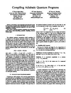
FIG. 3: (Color online) Number of “unsolved” problem instances as a function of the number of iterations. All instances were solved within 13 iterations.

global minimum, in addition to correcting for some of the single bit flip deviation from |M 0 i. The adiabatic time (2) can be computed using QMC in the same manner as described in [24]. If on an iteration, the adiabatic time is small enough to be computed accurately and is found to be < 16 µs, or the probability of states in the well of the global minimum just before a perturbative crossing is > 0.005, the instance is considered solved on that iteration. This is because the probability of finding the global minimum at least once in the 500 computations of the iteration is then > 92%. The “feasible range” of ∆i values, as mentioned in the algorithm description, was chosen to be between 1/4 and 8. More specifically, on each iteration, the ∆i values would always be scaled such that the smallest was 1/4, and the other ∆i values rarely approached 8, especially after several iterations, where most ∆i values were < 4. Beyond just testing whether the algorithm presented here is successful or not, it is critical to gain insight into how the changes in ∆i values affect the evolution of the ground state. Although a 264 -dimensional system cannot feasibly be examined in detail, much can be seen by examining the ground state expectation values (i) (i) hσz i ≡ h0|σz |0i of the 64 operators, i.e., the average magnetization of each qubit in the instantaneous ground state. Figure 2 illustrates these expectation values as a function of s for 4 iterations of the algorithm with an example instance. In each of the 4 plots, 64 horizontal (i) strips color-code the value of hσz i for all 64 qubits, during the evolution, calculated using QMC sampling. At s = 0, the ground state is a uniform superposition of all (i) computation states, so hσz i = 0 (green), and at s = 1, the ground state is the global minimum of HP , there(i) fore hσz i = ±1 (red/blue) depending on the state of the qubit. Moving away from s = 0, the expectations grad-

[1] E. Farhi, J. Goldstone, S. Gutmann, J. Lapan, A. Lundgren, and D. Preda., Science, 292, 472 (2001).

ually tend toward −1 or +1 as the ground state settles into global or local minima. If the system directly settles into the global minimum (as in iteration 4), then there (i) will be a continuous change of hσz i from 0 to their ultimate values with no sharp transition. If, on the other hand, the system initially settles into some cluster of local minima, then a sudden change is expected at the anticrossing between the eigenstates corresponding to the local and global minima (|M 0 i and |M i). Iterations 0-3 clearly show such sudden transitions. After each iteration, the anticrossing moves to an earlier time, though this was not general among all the instances examined. In the last iteration, the anticrossing is completely removed and the transition from the beginning to the end state is smooth. All 50 of the extremely difficult 64-node random instances were solved within 13 iterations of the algorithm. The number of unsolved instances after each iteration is plotted in Fig. 3. Among the instances, 30 of them were solved in 2 iterations, and all but 1 were solved in 10 iterations, with an overall average of 3.0 iterations required. These data suggest that the selection of β to ensure equal application of penalties is quite robust at remembering previous penalties while still applying new penalties.

VII.

CONCLUSIONS

We have demonstrated that a simple adiabatic quantum algorithm, based on penalization of paths to clusters of local minima by tuning single-qubit tunnelling energies, is effective at eliminating extremely small gaps caused by perturbative crossings. We presented a method for generating 64-qubit random instances of maximum independent set with 105 to 106 highly degenerate local minima and a unique global minimum, causing perturbative crossings between the two. It is found that even for these instances, the algorithm can eliminate the perturbative crossings in a small number of iterations.

Acknowledgements

The authors are grateful to B. Altshuler, P. Bunyk, E. Chapple, P. Chavez, E. Farhi, S. Gildert, F. Hamze, R. Harris, M. Johnson, T. Lanting, K. Karimi, H. Katzgraber, T. Mahon, T. Neuhaus, R. Raussendorf, C. Rich, G. Rose, M. Thom, E. Tolkacheva, B. Wilson, and A.P. Young for useful discussions. The authors also thank the volunteers of the AQUA@home project, who donated their computing resources to run the QMC simulations for this work.

[2] D. Aharonov, W. van Dam, J. Kempe, Z. Landau, S. Lloyd, and O. Regev, Proceedings of the 45th FOCS, p.

7 42 (2004). [3] Ari Mizel, D.A. Lidar, and M. Mitchell Phys. Rev. Lett. 99, 070502 (2007). [4] M.H.S. Amin, P.J. Love, and C.J.S. Truncik, Phys. Rev. Lett. 100, 060503, (2008); M.H.S. Amin, C.J.S. Truncik, and D.V. Averin, Phys. Rev. A 80, 022303 (2009). [5] W. van Dam, M. Mosca, and U. Vazirani, Proc. 42nd FOCS, 279 (2001). [6] M. Znidaric and M. Horvat, Phys. Rev. A 73, 022329 (2006). [7] J. Roland and N.J. Cerf, Phys. Rev. A 65, 042308 (2002). [8] M.H.S. Amin, V. Choi, Phys. Rev. A 80, 062326 (2009). [9] B. Altshuler, H. Krovi and J. Roland, Proceedings of the National Academy of Sciences of the USA, 107, 12446 (2010); eprint arXiv:0908.2782 . [10] E. Farhi, J. Goldstone, D. Gosset, S. Gutmann, H.B. Meyer, P. Shor, [11] Neil Dickson, M.H.S. Amin, Phys. Rev. Lett. 106, 050502 (2011). [12] A.P. Young, S. Knysh, V.N. Smelyanskiy, Phys. Rev. Lett. 104, 020502 (2010). [13] T. J¨ org F. Krzakala, G. Semerjian, and F. Zamponi, Phys. Rev. Lett. 104, 207206 (2010). [14] L. Foini, G. Semerjian, and F. Zamponi, Phys. Rev. Lett. 105 167204 (2010). [15] T. Neuhaus, M. Peschina, K. Michielsen, and H. De Raedt, Phys. Rev. A 83, 012309 (2011). [16] V.Choi, Quant. Inf. Comput. 11, 0638 (2011); eprint arXiv:1010.1220.

[17] S. Knysh, V. Smelyanskiy, eprint arXiv:1005.3011. [18] P. Crescenzi and A. Panconesi, Lecture Notes in Computer Science 380, (1989) [19] M.S. Sarandy and D.A. Lidar, Phys. Rev. A 71, 012331 (2005); Phys. Rev. Lett. 95, 250503 (2005). [20] L. Ingber, Mathematical and Computer Modelling 18, 11 (1993). [21] T. Cormen, C. Leisersen, R. Rivest, C. Stein, Introduction to Algorithms (2nd ed.), MIT Press and McGrawHill, (2001). [22] R. Harris, M.W. Johnson, T. Lanting, A.J. Berkley, J. Johansson, P. Bunyk, E. Tolkacheva, E. Ladizinsky, N. Ladizinsky, T. Oh, I. Perminov, C. Enderud, C. Rich, S. Uchaikin, M.C. Thom, E.M. Chapple, J. Wang, B. Wilson, M.H.S. Amin, N. Dickson, K. Karimi, B. Macready, C.J.S. Truncik, and G. Rose, Phys. Rev. B 82, 024511 (2010). [23] M.W. Johnson, M.H.S. Amin, S. Gildert, T. Lanting, F. Hamze, N. Dickson, R. Harris, A.J. Berkley, J. Johansson, P. Bunyk, E.M. Chapple, C. Enderud, J.P. Hilton, K. Karimi, E. Ladizinsky, N. Ladizinsky, T. Oh, I. Perminov, C. Rich, M.C. Thom, E. Tolkacheva, C.J.S. Truncik, S. Uchaikin, J. Wang, B. Wilson, and G. Rose, Nature 473, 194 (2011). [24] K. Karimi, N. G. Dickson, F. Hamze, M.H.S. Amin, M. Drew-Brook, F.A. Chudak, P.I. Bunyk, W.G. Macready, and G. Rose, arXiv:1006.4147v4.