Experimental Investigation of Flow Field Around An ...

AIAA 2017-3501 AIAA AVIATION Forum 5-9 June 2017, Denver, Colorado 23rd AIAA/CEAS Aeroacoustics Conference

On The Flow Field and Aerodynamic Sound Emission Around An Asymmetric Beveled Trailing Edge Yaoyi Guan∗ University of Notre Dame, Notre Dame, IN, 46556, United States

Scott C. Morris†

Downloaded by Yaoyi Guan on June 26, 2017 | http://arc.aiaa.org | DOI: 10.2514/6.2017-3501

University of Notre Dame, Notre Dame, IN, 46556, United States The velocity field and unsteady surface pressure field around the trailing edge section of an airfoil was studied experimentally. The aerodynamic sound generated by the trailingedge flow was determined experimentally by beamforming technique. The airfoil geometry considered was a flat strut upstream of the trailing edge section providing canonical, zeropressure-gradient, turbulent boundary layers. The geometry of the beveled trailing edge section was defined by the ratio of curvature to airfoil thickness, 𝑅/𝑇 , and the trailing edge angle 𝜃. The Reynolds number based on the chord was 2.1 × 106 . The velocity field in the near wake was measured by Particle Image Velocimetry (PIV) to provide insight into the characteristics of unsteady surface pressure field around the trailing edge. Characteristic statistics of the unsteady surface pressure field were obtained by arrays of Remote Microphone Probes (RMP) for understanding of the physical process of sound scattering. The spanwise correlation length of the unsteady surface pressure under separated shear layer was estimated from experimental data. The spanwise cross-correlation of the upperand lower-surface pressure fluctuations was modeled. The simplified half-plane theory for sound prediction was modified to incorporate the contribution from the coupling of the upper- and lower-surface pressure fluctuations. The prediction showed good agreement to experimental data.

Nomenclature 𝑐 airfoil model chord 𝑓 frequency 𝐿3 model span 𝑀∞ free stream Mach number 𝑀𝑐 convection velocity Mach number 𝑞∞ dynamic pressure 𝑅 radius of curvature 𝑅𝑒 Reynolds number 𝑇 airfoil thickness 𝑢𝑐 convection velocity 𝑢∞ free stream velocity Δ𝑧 spanwise spatial separation 𝛿 boundary layer thickness 𝛿∗ boundary layer displacement thickness 𝛾3 spanwise coherence ∫∞ Λ3 spanwise integral length scale, Λ3 (𝑓 ) = 0 𝛾3 (𝑓, Δ𝑧) dz Φ𝑝𝑝 autospectral density of the unsteady surface pressure Φ𝑃𝑟𝑎𝑑 autospectral density of the radiated sound ∗ Postdoc

Research Associate, Department of Aerospace and Mechanical Engineering, [email protected]. Department of Aerospace and Mechanical Engineering, AIAA member.

† Professor,

1 of 15 American Institute of Aeronautics and Astronautics Copyright © 2017 by the American Institute of Aeronautics and Astronautics, Inc. All rights reserved.

𝜙 𝜑 𝜔

azimuthal angle of coordinate system zenith angle of coordinate system angular frequency


I.

Introduction

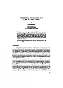
The characteristics of the velocity and unsteady surface pressure (USP) field around the trailing edge section of an airfoil together with the aerodynamic sound generated by the trailing-edge flow are presented in this paper. The experiments for present study employed Particle Image Velocimetry (PIV) to obtain twocomponent velocity statistics of the flow field, arrays of remote microphone probes (RMP) to measure the unsteady surface pressure and phased array of microphones to determine the far-field aerodynamic sound. The experimental data were utilized to provide insight into the aerodynamic sound emission induced by trailing-edge flows. The applicability of half-plane theory, which is utilized to predict flow-induced trailingedge noise based on statistics of the flow field, was tested under complex flow conditions and validated against experimental data. The cross-correlation of the upper- and lower-surface pressure fluctuations was studied and incorporated into the prediction of trailing-edge noise. These results are of great interest for the understanding and estimation of aerodynamics sound generated by turbulent flow over non-compact lifting surface.1, 2 For example, cooling fans, wind turbine blade and propellers can generate considerable aerodynamic noise.3 In these applications, the trailing-edge noise dominates all other structural-acoustic sources.4 As a result, understanding of the mechanism of trailing-edge noise emission and estimation of the sound pressure level are of paramount importance for the design of quiet lifting surfaces. The original theory for aerodynamic sound generated as a byproduct of an fluid flow, which is distinct from sound produced by the vibration of solids, was proposed by Lighthill.1, 2 This theory is based on the analogy between nonlinear flow theory and linear acoustic theory. Curle5 assumed spherical propagation and applied free space Green’s function in the presence of an arbitrary body, which is acoustically compact, to yield an expression of the free-field sound by solving Lighthill’s equation. Ffowcs Williams and Hawkings6 derived a general formula from Lighthill’s analogy for the far-field sound pressure produced by the flow over an arbitrary surface. Powell7 derived a formulation of the acoustic pressure generated by a turbulent flow based on the vorticity-velocity interactions. Howe8 presented an alternative form of this formula by linearizing the equation. A more fascinating aspect of aerodynamic noise is the sound scattered by the trailing edge of the body immersed in flow. This occurs when the chord is comparable with or exceeds the acoustic wavelength and is the source of intense broadband noise. The trailing-edge noise, which is often the dominant source of aerodynamic sound generated by lifting surface with large chord, was studied intensively by both experiments and theories.3, 9–14 In these studies, the flows around the trailing edge section of a lifting surface was regarded as the sound source. Therefore, the characteristics of the trailing-edge flow are of great interest for understanding of the trailing-edge noise generation. Early work on the trailing-edge flows has been reported by Blake. Blake and co-workers15–17 introduced a class of asymmetrical beveled trailing edges with uniform flat lower surfaces in order to systematically study trailing edge flows. The members of this class can be characterized by the trailing edge angle, 𝜃, and the ratio of radius of curvature of the rounded part 𝑅 to the plate thickness 𝑇 as shown in Fig. 1. The velocity fields and unsteady surface pressure fields around three trailing edge geometries were measured experimentally.15, 16 The change in trailing edge angle (𝜃) resulted in large difference in flow fields. The geometry with larger trailing edge angle (𝜃 = 45∘ ) produced strong vortex shedding with constant shedding frequency. Later, flow fields around Blake’s trailing edges were studied both experimentally18–20 and numerically.21, 22 More recently, the flow fields around a family of asymmetrically beveled trailing edges with 25∘ trailing edge angle and various 𝑅/𝑇 values were studied.23–26 These studies showed that the characteristics of the flow fields were highly dependent on the geometric parameter (𝑅/𝑇 ). Small variation in 𝑅/𝑇 could induce large change in flow features. Pröbsting et al.20 studied the characteristics of the trailing-edge flow around a 45∘ trailing edge and the radiated far-field sound. The discrepancy between prediction and experimental data of far-field sound showed that the simplified wake model and diffraction theory was not generally applicable. On the other hand, the prediction of sound based on the unsteady surface pressure near the trailing edge, which was evaluated from the velocity field measured by tomographic PIV, compared favorably with the reference measurements.27 This results kept consistent with previous theoretical work4, 10, 28 which argued that the pressure fluctuations

2 of 15 American Institute of Aeronautics and Astronautics

−5

−4

−3

−2

−1

0

1

p−p∞ 2 1/2ρU∞

0 −0.2 −0.4 −0.6 FPG

APG

Reverse flow

−0.8 1.5


y/T

1 0.5

T

R yf

0 −0.5

−5

−4

−3

−2

−1

0

1

x/T

Figure 1. Parametric representation of the beveled trailing edge geometry, static pressure distribution; ∘; streamwise mean velocity profiles, ; contour of strreamwise root-mean-square velocity.

were scattered at the discontinuity posed by the trailing edge, which could be the dominating noise sources at low Mach numbers, and the radiated sound could be estimated based on the statistics of the unsteady surface pressure near the trailing edge. As a result, the characteristics of unsteady surface pressure under complex flows are of scientific interest in order to estimate the trailing-edge noise as the trailing-edge flows are often under strong non-equilibrium conditions, including favorable/adverse pressure gradients, separation and recirculation (as shown in Fig. 1). The characteristics of the USP under turbulent boundary layer with zero pressure gradient (ZPG) have been studied analytically, experimentally and numerically for over 60 years.29–33 Goody34 extensively reviewed previously published experimental data over large range of Reynolds numbers and proposed an empirical model for the unsteady surface pressure spectrum under turbulent boundary layer with ZPG incorporating the Reynolds number effect. Observing that low- and high-frequency fluctuations show a better scaling behavior with the outer and inner scales of the boundary layer, respectively, Goody introduced a Reynolds number dependence through a parameter Re𝑇 , the ratio of the outer and inner time scales in the boundary layer. The model is given by the following expression, with 𝑢𝑒 the local edge velocity and 𝜏𝑤 the wall shear stress: 3.0(𝜔𝛿/𝑢𝑒 )2 Φ𝐺𝑜𝑜𝑑𝑦 (𝜔)𝑢𝑒 = . (1) 2 −0.57) 7 𝜏𝑤 𝛿 [(𝜔𝛿/𝑢𝑒 )0.75 + 0.5]3.7 + [(1.1𝑅 ] (𝜔𝛿/𝑢𝑒 ) 𝑇

Studies were performed on the USP under turbulent boundary layer with pressure gradients.35–38 Simpson et. al. studied the characteristics of the surface pressure fluctuation in a separating turbulent boundary layer39 experimentally. The unsteady surface pressure on steps immersed in turbulent boundary layers were studied numerically40 and experimentally,41 respectively. The characteristics of the unsteady surface pressure over asymmetrically beveled trailing edges were studied experimentally.4, 42 Despite the extensive studies on the characteristics of the unsteady surface pressure under various complex flow conditions, the prediction of trailing-edge noise based on the statistics of unsteady surface pressure is still questionable because of the limitation on the assumptions and interpretations of the theories.4, 13, 28 Amiet43 determined the far-field radiated sound scattered by an airfoil when an incident vortical velocity



field impinges on the leading edge of an airfoil. A theoretical expression for the far-field sound spectra was given in terms of auto-spectral density and spanwise correlation length of the upwash velocity. Later, Amiet28 extended his theory to apply to the case of noise produced by turbulent flow past the trailing edge of an airfoil. The far-field sound was expressed as a function of the hydrodynamic wall pressure convected past the trailing edge and the spanwise correlation length of the unsteady surface pressure. Howe10 expressed the aerodynamics sound generated by the interaction of low Mach number turbulent flow with the edge of a semi-infinite rigid plate analytically as a function of the unsteady surface pressure near the trailing edge. Blake4 utilized Howe’s theory incorporated with a half-plane Green’s function to predict the sound generated by a sharp trailing edge based on the statistics of the USP near the trailing edge. The inputs for Blake’s formulation include the frequency-dependent spanwise correlation length Λ3 and the auto-spectral density of the USP, Φ𝑝𝑝 . Blake’s formulation was utilized to predict the broadband noise generated by turbulent boundary layer convecting over the flat lower surface of an asymmetrically beveled trailing edge and showed good agreement to experimental results.44 Note that all the aforementioned theories were derived based on the statistics of attached turbulent flow convecting over one single side of a rigid surface. Moreover, the convecting turbulence over the surface was assumed to be statistically stationary along streamwise direction. However, most of the trailing-edge flows were non-equilibrium in engineering applications and flow separation may occur near the trailing edge. The convecting turbulence on either side of the trailing edge contribute to the far-field aerodynamic sound. In present study, the applicability of the half-plane theory for predicting the trailing-edge noise based on the statistics of the unsteady surface pressure is considered using detailed measurements of both the USP under inhomogeneous, separated flow and radiated sound scattered by an asymmetrically beveled trailing edge. The velocity fields around the trailing edge were also measured for understanding the underlying physics of sound emission.

II.

Experimental Method

The airfoil model in present study was constructed as a flat strut with a uniform cross section across the span. The cross section of the leading edge component of the airfoil model was a semi-ellipse with five-to-one aspect ratio. The mid section of the airfoil model was a flat plate with uniform thickness of 𝑇 = 5.08𝑚𝑚. The lower surface of the trailing edge section was flat. The tip angle of the trailing edge was 25∘ . The horizontal and slanted flat part of the upper surface was connected tangentially by a circular arc with radius 𝑅. The value of the geometric parameter 𝑅/𝑇 was 4. The cross-section of the trailing edge part of the airfoil model was shown in Fig. 1. Both the upper- and lower-surface flow were tripped at the location quarter chord downstream of the leading edge. The boundary layer thickness (based on 99% of the free-stream velocity) and the displacement thickness at 𝑥/𝑇 = −5.5 were found to be 𝛿 = 8.6mm and 𝛿 ∗ = 1.2mm, respectively, as measured by a single-sensor hot-wire anemometer. The velocity fields around the trailing edge section of the airfoil model was measured by both conventional, planner PIV and high-speed, time-resolved PIV. The reader is referred to Guan et al.24 for a detailed description of the experimental setup. The measurement of the unsteady surface pressure and far-field sound presented in this study were conducted in Anechoic Wind Tunnel (AWT) facility at the University of Notre Dame. The AWT consists of an open-jet test section surrounded by a large anechoic chamber, whose walls are covered with glass fiber wedges rated with an absorption coefficient of 99% for 𝑓 > 100Hz. Air is drawn in through a set of turbulence screens, a 8:1 contraction, and a straight section to the nozzle exit with cross section 0.61m × 0.61m. The flow in the test section was constrained on the upper and lower sides by end plates to eliminate finite span effects and to ensured a 2D mean flow. Two shear layers were formed by the flow exiting the inlet on the unconstrained sides of the test section, which created a two-sided open jet allowing for the propagation of the trailing edge sound to the surrounding anechoic room. The airfoil model was mounted vertically at zero incidence in the test section such that the upstream part of the model, up to the quarter-chord point, was placed inside the straight section in order to avoid influence of the growing free-shear layers on the flow near the trailing edge. At the opposite side of the chamber, the flow was guided through an acoustically treated diffuser section to the primary fan.45, 46 Figure 2 shows a schematic of the AWT. Measurements of the USP were acquired by arrays of remote microphone probes (RMP), which were flush mounted on the surface of the airfoil model. The structure of the RMP and the method of calibration were described in detail by Guan et al.47 Identical technique was employed to measure the surface pressure


Screen and honey comb Acoustic baffle

Microphone array

Model Inlet

Outlet

End plate

Microphone array Acoustic wedges

Fan room


Figure 2. Schematic of the Anechoic Wind Tunnel facility with installation of the airfoil model and phased microphone arrays.

Figure 3. Illustration of RMP array over the upper surface of the airfoil trailing edge (not on scale).

fluctuations in trailing-edge flows and flow over backward-facing step.23, 41 The unsteady surface pressure around the trailing edge section of the airfoil was measured by a streamwise array of 8 RMP on the lower surface and a T-shaped array of 14 RMP on the upper surface of the trailing edge. The distribution of the RMP array over the upper surface of the airfoil model is shown in Fig. 3. The dark gray surface is the cross-section of the two-dimensional airfoil. The RMP array locates in the middle span of the airfoil. Two large aperture phased arrays were utilized to measure the sound generated by the trailing edge. On each phased array, 40 condenser microphones were arranged in a logarithmic spiral configuration.48 The two phased microphone arrays were placed parallel to the centerline of the wind tunnel at a distance of 2.38m and had its center aligned with the trailing edge of the airfoil model as shown in Fig. 2. Data was acquired at a frequency of 40kHz with 64 ensembles in total. Each ensemble contained 32,768 samples. More details of the characteristics of the phased arrays utilized in present study were described and discussed by Shannon and Morris.44 Three beamforming methods were utilized in present study to process the experimental data of sound measurement including the delay-sum,49 the weighted Cross Spectral Matrix (CSM)50 and the Deconvolution Approach for the Mapping of Acoustic Sources (DAMAS).51


III.


A.

Results and Discussion

Characteristics of flow field

As outlined in the introduction, the statistical characteristics of the turbulent flow features are closely linked to the unsteady surface pressure and aerodynamic sound generation. Therefore, the velocity field was obtained by PIV measurement to provide detailed information regarding the statistical properties of the flow features and the length scales as well as quantitative visualization of the flow structure to supports the interpretation of the unsteady surface pressure and acoustics measurements. The static pressure distribution over the upper surface of the trailing edge and the contour of the normalized streamwise room-mean-square √ ′2 velocity, 𝑢 /𝑢∞ , around the trailing edge are shown in Fig. 1. The contour of the instantaneous spanwise vorticity components 𝜔𝑧 = (∂𝑣/∂𝑥 − ∂𝑢/∂𝑦)𝑇 /2𝑢∞ are shown in Fig. 4. The turbulent boundary layer on the lower flat surface remained almost streamwise invariant up to the trailing edge. The lower-surface flow separated at the tip of the trailing edge. A thin free shear layer developed from the separation point at the edge. The upper-surface flow experienced complex flow conditions. The upper-surface flow accelerated in the favorable pressure gradient region up to 𝑥/𝑇 = −2.75. Downstream of FPG region, the thickness of the turbulent boundary layer was observed to increase dramatically on the upper surface as a result of the severe adverse pressure gradient as shown in Fig. 1. Unsteady separation occurred around 𝑥/𝑇 = −1.1 and 𝑦/𝑇 = 0.5. As already pointed out by Simpson et al.,39 this separation point was not stationary, but shifted upstream and downstream over time. A free shear layer developed from the upper-surface separation point. A recirculation region was bounded by the rigid surface of the airfoil and the upper-surface free shear layer. Downstream of the trailing edge, the two free shear layers developed without interaction up to 𝑥/𝑇 = 2 as shown in Fig. 4. Only further downstream, at 𝑥/𝑇 > 2, large-scale coherent structures were observed in the vorticity field. Guan et al.24 showed that the scale of the coherent structures in the far wake was proportional to the wake thickness, 𝑦𝑓 , which is defined as the minimum vertical distance between the two local maxima of the streamwise root-mean-square velocity in the lower and upper shear layers in the wake as shown in Fig. 1.4 The interpretation of 𝑦𝑓 was discussed by Pröbsting et al.20 More detailed, quantitative description of the flow field was provided by Guan et al.24 It should be noted that the upper-surface shear layer was observed to be correlated to the turbulent wake while the lower-surface boundary layer was not correlated to the wake.24 B.

Characteristics of USP field

The unsteady surface pressure was measured using arrays of RMP on both sides of the trailing edge section. The auto-spectral densities of the USP are presented in this section. The spectral density was estimated using the average modified periodogram method of Welch.52 Time series segments with a length of 4, 096 samples and a Hamming windowing function was applied and the average was computed with an overlap of 50% over a total number of 1, 023 windows, resulting in a frequency resolution of Δ𝑓 = 9.8Hz. Fig. 4 shows the autospectral density of the unsteady surface pressure on the upper and lower surface in the left and right subfigures, respectively. The USP autospectral density was normalized by freestream velocity 𝑢∞ , airfoil thickness 𝑇 and dynamic pressure 𝑞∞ . As the flow progressed downstream over the curved upper surface, the spectral magnitude of the USP increased about 15dB at 𝑓 𝑇 /𝑢∞ = 0.3 as shown in Fig. 4 (a). This is because the most downstream measurement point located under the separated shear layer, where large-scale turbulent motions associated with low-frequency oscillations occurred. In contrast, the spectral magnitude of the USP at 𝑓 𝑇 /𝑢∞ = 6 was observed to drop over 20dB within the same spatial domain as flow moving downstream. The decrease is attributed to the rapid drop of the wall shear and the increasing distance between the wall and the fluctuation-producing structures in the free shear layer. Guan and Morris42 presented detailed information about the scaling of the upper-surface pressure fluctuations under separated shear layer. The characteristics of the upper-surface pressure fluctuations under separated flow showed great variety and were dominated by various flow regimes in different frequency ranges. The low-frequency spectral magnitude of the USP under separated flow were dominated by the turbulent motions in the local shear layer. However, the frequency of the large-scale oscillations was governed by the turbulent wake. The middle-frequency range of the USP was dominated by the characteristics of the local shear layer. The high-frequency components of the USP spectral density was mainly influenced by the upstream-convecting turbulence created by reverse flow.


y/T

2

2

1

1

0

0

−1

ωz T u∞

−2

−2

−10

0

10 −1

0 2

−2

4

−2

0

x/T Boundary layer induced pressure

−4

Φpp (f)u∞ 2 T q∞

10


2

4

x/T Boundary layer induced pressure

−6

10

Pressure fluctuations modulated by the wake

a)

−8

10

Wake induced pressure

−1

10

b) 0

10 fT /u∞

1

10

−1

10

0

10 fT /u∞

1

10

Figure 4. The autospectral density of unsteady surface pressure on the a) upper and b)lower surface of the trailing edge

The streamwise evolution of the USP on lower surface is shown in Fig. 4 (b). The spectral magnitude of the USP in the frequency domain 𝑓 𝑇 /𝑢∞ > 2 at different streamwise locations showed very limited variation. This is because the high-frequency pressure fluctuations were dominated by the attached turbulent boundary layer, which remained almost invariant along the streamwise direction as shown by the PIV measurements. Note that the spectral magnitude at the location closest to the trailing edge in high frequency range decreased about 1dB compared with that measured at the most upstream location. This was caused by the decrease in the wall shear as well as the slight increase in the boundary layer thickness along the downstream direction, which resulted from a slight adverse pressure gradient created by the small high-pressure region close to the trailing edge. In contrast, the energy content of the low-frequency components (𝑓 𝑇 /𝑢∞ ≤ 2) showed a large increase closer to the trailing edge. This indicates that the low-frequency oscillation of the surface pressure was dominated by the contribution from the large-scale turbulent motions in the wake.21 Since the turbulent wake and the lower-surface boundary layer were uncorrelated as shown by the PIV measurement,24 the auto-spectral density of the lower-surface USP, Φ𝑝𝑝 −𝑙𝑜𝑤𝑒𝑟 , can be written as Φ𝑝𝑝 −𝑙𝑜𝑤𝑒𝑟 = Φ𝑍𝑃 𝐺 + Φ𝑤𝑎𝑘𝑒 .

(2)

where Φ𝑍𝑃 𝐺 represents the USP spectral density that would exist in a canonical turbulent boundary layer with zero pressure gradient and Φ𝑤𝑎𝑘𝑒 represents the contribution of the wake. In present study, an empirical model for predicting the wake-induced wall pressure fluctuations was proposed based on scaling of the experimental data as Φ𝑤𝑎𝑘𝑒 𝑢∞ 𝑟2 𝐶1 (𝑓 𝑦𝑓 /𝑢∞ )𝐴1 = . 𝑞∞ 2 𝑦𝑓 𝑦𝑓 2 [(𝑓 𝑦𝑓 /𝑢∞ )𝐴2 + 𝐶2 ]𝐴3

(3)

where 𝑢∞ is the free-stream velocity, 𝑞∞ is the dynamic pressure, 𝑦𝑓 is the wake thickness and 𝑟 is the distance between the observation point and center of the distributed fluctuation-producing sources. A least-square approximation to all of the data resulted in the constants 𝐴1 = 0.38, 𝐴2 = 1.74, 𝐴3 = 2.77, 𝐶1 = 8.18×10−7 , and 𝐶2 = 0.0857. Values obtained from this representation, in combination with Goody’s34 7 of 15 American Institute of Aeronautics and Astronautics

−4

10

−5

Φpp (f)u∞ 2 T q∞

10

−6

10

−7

10

−8

10

−1

10

0

10 f T/u∞

10

1


Figure 5. Comparison of the predicted lower-surface USP auto-spectral density and experimental data, ∘, Φ𝑝𝑝 −𝑙𝑜𝑤𝑒𝑟 experimental data; , Φ𝑍𝑃 𝐺 predicted by Goody’s34 model; , Φ𝑤𝑎𝑘𝑒 predicted by wake model; , Φ𝑝𝑝 −𝑙𝑜𝑤𝑒𝑟 , predicted by Equation 2.

model and equation 2, allow for an accurate representation of the lower-surface pressure spectral magnitude at specified streamwise locations. As a demonstration of this, Figure 5 shows a detailed comparison of the predicted pressure fluctuations with the USP measured at the location closest to the trailing edge on the lower surface. The prediction showed agreement with the experimental data. The discrepancy in low frequency range between the prediction and experimental data was within the uncertainty range of ±3dB. The high-frequency spectral magnitude was overestimated. This is because Goody’s model was applied to the cases without pressure gradient while a slight adverse pressure gradient existed on the lower surface near the trailing edge in present study as discussed. In addition to the overall spectral magnitude of the USP, the estimation of far-field sound requires the ∫ ∞ specification of the spanwise correlation length scale of the USP, which can be computed as Λ3 (𝑓 ) = 𝛾3 (𝑓, Δ𝑧)𝑑𝑧. The spanwise coherence was obtained from the USP data collected by the spanwise array on 0 the upper surface of the trailing edge and is shown in Fig. 6. The frequency is normalized by spanwise spatial separation Δ𝑧 and convection velocity 𝑢𝑐 with the assumption of 𝑢𝑐 = 0.6𝑢∞ . The open symbol represents the experimental data. The red dashed line represents the prediction of the spanwise coherence of USP 𝜔Δ𝑧 under turbulent boundary layer without pressure gradient by the Corcos’ model30 (𝛾𝑧 = 𝑒−𝛼∣ 𝑢𝑐 ∣ , 𝛼 = 0.7). The black dashed line represents the prediction by the Corcos’ model with 𝛼 = 0.4. Note that the value of spanwise coherence of USP under separated shear layer was larger than that for the USP under turbulent boundary layer without pressure gradients. This is because the spanwise scale of the turbulent structures in the free shear layer is larger than that in the attached turbulent boundary layer and the resulting spanwise correlation length is larger. Fig. 7 shows the spanwise coherence of the upper- and lower-surface pressure fluctuations (𝛾𝑢𝑙 ), which is represented by the red curve. The frequency is normalized by spanwise spatial separation Δ𝑧 and convection velocity 𝑢𝑐 . The value of Δ𝑧 is larger than 2𝑐𝑚 in present study. Better spatial resolution can not be achieved because of the limited spacing for RMP array. The spanwise coherence of the upper-surface USP (𝛾𝑢 ) is represented by the black curve for comparison. The non-zero coherence between the upper- and lower-surface USP indicates that they are correlated. The value of 𝛾𝑢𝑙 decreases with increasing 𝑓 Δ𝑧/𝑢𝑐 as expected. The decay rate of (𝛾𝑢𝑙 ) with respect to (𝑓 Δ𝑧/𝑢𝑐 ) is almost identical to that of (𝛾𝑢 ) in the domain 𝑓 Δ𝑧/𝑢𝑐 < 0.75. As 𝑓 Δ𝑧/𝑢𝑐 > 0.75, the value of 𝛾𝑢𝑙 decreases sharply. This is because the low-frequency oscillations of the lower-surface USP are dominated by the turbulent wake. The low-frequency oscillation of the upper-surface pressure fluctuations are influenced by the shear layer and modulated by the wake. As a result, the upper- and lower-surface pressure fluctuations are correlated in low frequency range. On the other hand, the high-frequency components of the upper-surface pressure fluctuations are dominated by the reverse flow. Therefore, the high-frequency USP on the lower surface, which is dominated by the lower-surface attached turbulent boundary layer, is not correlated to the high-frequency upper-surface USP. For modeling the spanwise coherence of the upper- and lower-surface USP, the pressure fluctuations on the lower surface are assumed to be composed by two parts as shown in Fig. 5. The turbulent boundary 8 of 15 American Institute of Aeronautics and Astronautics

1 0.8

γ

0.6 0.4 0.2


0 0

0.5

1

1.5

f ∆z/uc Figure 6. Spanwise coherence of USP under separated shear layer on the upper surface of the trailing edge, ∘, experimental data; , predicted coherence of USP from Corcos’ model with 𝛼 = 0.4; , Corcos’ model for coherence of USP under turbulent boundary layer without pressure gradients.

layer-induced USP on the lower surface is not correlated to the upper-surface pressure fluctuations since the lower-surface flow is not correlated to the wake or the upper-surface shear layer. The coherence between the wake-induced lower-surface pressure fluctuations and the USP on the upper surface is assumed to be expressed in Corcos’ model as 𝜔Δ𝑧 𝛾𝑝𝑤𝑎𝑘𝑒 𝑝𝑢 = 𝑒−𝛼∣ 𝑢𝑐 ∣ . (4) As a result, lower-surface USP is only partially correlated to the upper-surface USP. Consider the crossspectral density of the upper- to lower-surface pressure fluctuations, which can be written as Φ𝑝𝑙 𝑝𝑢 = 𝑝ˆ𝑙 𝑝ˆ 𝑢

∗

(5)

whereˆrepresents Fourier Transform, ∗ represents complex conjugate and the overline represents ensemble average, 𝑝𝑢 and 𝑝𝑙 represent the upper- and lower-surface pressure fluctuations, respectively. According to Equation 2 and zero correlation between turbulent boundary layer-induce pressure fluctuations on lower surface and upper-surface USP, Φ𝑝𝑙 𝑝𝑢 can be expressed as Φ𝑝𝑙 𝑝𝑢 = 𝑝ˆ𝑙 𝑝ˆ 𝑢

∗

= (𝑝ˆ 𝑝𝑢 𝑤𝑎𝑘𝑒 + 𝑝ˆ 𝑍𝑃 𝐺 )ˆ ∗

∗

= 𝑝ˆ ˆ ˆ 𝑤𝑎𝑘𝑒 𝑝 𝑢 + 𝑝ˆ 𝑍𝑃 𝐺 𝑝 𝑢 ˆ = 𝑝ˆ 𝑤𝑎𝑘𝑒 𝑝 𝑢

∗

(6)

∗

= Φ𝑝𝑤𝑎𝑘𝑒 𝑝𝑢 . Equation 6 indicates that the cross-spectral density of upper- to lower-surface USP is equal to the crossspectral density of wake-induced pressure fluctuations to upper-surface USP. If the ratio of spectral magnitude of Φ𝑍𝑃 𝐺 to that of Φ𝑤𝑎𝑘𝑒 is expressed as a frequency-dependent factor 𝜆(𝑓 ) = Φ𝑍𝑃 𝐺 (𝑓 )/Φ𝑤𝑎𝑘𝑒 (𝑓 ),

(7)

the auto-spectral density of lower-surface USP can be written as Φ𝑝𝑙 = Φ𝑤𝑎𝑘𝑒 + Φ𝑍𝑃 𝐺 = (1 + 𝜆)Φ𝑤𝑎𝑘𝑒 .


(8)

0.4 γ3, upper− to lower−surface USP γ , upper−surface USP 3

γ3

0.3

0.2

0.1


0 0.2

0.4

0.6

0.8 1 f ∆z/uc

1.2

1.4

Figure 7. The spanwise coherence of pressure fluctuations with constant spatial separation Δ𝑧, of upper- and lower-surface USP; , coherence of upper-surface USP.

, coherence

The auto-spectral density of the upper-surface pressure fluctuations is ∗

Φ𝑝𝑢 = 𝑝ˆ ˆ 𝑢𝑝 𝑢 .

(9)

According to the definition of coherence, which is normalized cross-spectral density,53 the coherence of the upper- to lower-surface pressure fluctuations can be written as ∣Φ𝑝 𝑝 ∣ 𝛾𝑢𝑙 = √ 𝑢 𝑙 Φ𝑝𝑢 Φ𝑝𝑙

(10)

Substitute Equation 4 to 9 into Equation 10, 𝛾𝑝𝑙 𝑝𝑢 can be rewritten as ∣Φ𝑝 𝑝 ∣ 𝛾𝑢𝑙 = √ 𝑢 𝑙 Φ𝑝𝑢 Φ𝑝𝑙 ∣Φ𝑝𝑤𝑎𝑘𝑒 𝑝𝑢 ∣ (1 + 𝜆)Φ𝑤𝑎𝑘𝑒 Φ𝑝𝑢 1 =√ 𝛾𝑝𝑤𝑎𝑘𝑒 𝑝𝑢 1+𝜆 𝜔Δ𝑧 1 =√ 𝑒−𝛼∣ 𝑢𝑐 ∣ 1+𝜆 =√

(11)

The coherence of the upper- and lower-surface pressure fluctuations are computed as Equation 11 and shown in Fig. 8. Note that decay rate of the coherence between the upper-surface USP and the wake-induced USP on the lower side is assumed to be identical to the coherence decay rate for USP under upper-surface shear layer (𝛼 = 0.4). The predicted spanwise coherence of the upper-surface to lower-surface USP shows agreement to the experimental data. This non-zero cross-correlation of the upper- to lower-surface USP will be utilized to improve the prediction of trailing edge noise by Blake’s formulation.4 C.

Far-field sound

Prediction of aerodynamic sound requires detailed spatial-temporal information of the flow field around the solid body immersed in the fluid flow. Experimental methods are not able to provide adequate information for the prediction. Numerical simulation can be very expensive and time consuming. For simplifying the procedure of trailing-edge noise prediction, Blake4 derived a formulation predicting the far-field aerodynamic sound based on Howe’s theory10 and the half-plane Green’s function as Φ𝑃𝑟𝑎𝑑 (𝑢∞ /𝛿 ∗ ) 2 𝑞∞ 𝑀∞ (𝐿3 𝛿 ∗ /𝑟2 )𝑠𝑖𝑛2 (𝜑/2)∣𝑠𝑖𝑛(𝜙)∣

=

𝜔Λ3 𝑢𝑐 2 Φ𝑝𝑝 (𝑢∞ /𝛿 ∗ ) ( ) . 2 2 4𝛼𝜋 𝑢𝑐 𝑢∞ (𝜔𝛿 ∗ /𝑢∞ )𝑞∞


(12)

1

γpu pl

0.8 0.6 0.4 0.2 0

0

0.5

1

1.5


f∆z/uc Figure 8. Comparison of the predicted spanwise coherence of the upper- to lower-surface pressure fluctuations and the experimental data, , predicted 𝛾𝑢𝑙 ; ∘, experimental data.

Here a spherical coordinate system was employed to define the observer location, where 𝑟, 𝜑 and 𝜙 are the radial distance, azimuthal and zenith angle from the source to the far-field location, respectively. The dynamic pressure 𝑞∞ and freestream Mach number 𝑀∞ are determined by the free stream velocity 𝑢∞ . The convection velocity can be approximated as a constant fraction of freestream velocity (𝑢𝑐 = 0.6𝑢∞ ). The input for Blake’s formulation are the frequency-dependent spanwise correlation length Λ3 and the auto-spectral density of the unsteady surface pressure fluctuations Φ𝑝𝑝 . The value of 𝛼 is determined by the distance between the trailing edge and the location of USP measurement, 𝛼 = 1 as 𝜔Δ𝑥1 /𝑢𝑐 ≫ 1 while 𝛼 = 1/4 as 𝜔Δ𝑥1 /𝑢𝑐 ≪ 1. Note that Blake’s formulation predicts the sound generated by singlesided turbulence. Roger and Moreau13 suggested that the far-field sound spectra generated by two-sided turbulence over an airfoil should be expressed as the summation of the far-field sound spectra induced by the upper- and lower-surface pressure fluctuations, respectively, with the assumption that the the upperand lower-surface USP are not correlated. As a result, Equation 12 was utilized to compute the trailing-edge noise generated by the turbulence on either side of the airfoil. The summation of the noise from the upperand lower-surface source was regarded as the total noise propagated to the far-field. The prediction of farfield sound based on Blake’s formulation and Roger and Moreau’s assumption is represented by the red solid curve in Fig. 9, which is the summation of the sound generated by the lower- and upper-surface USP. The open circles represent the far-field sound measured experimentally by the phased microphone arrays. The data shown in Fig. 9 indicated that the far-field sound were dominated by the upper-surface USP in low frequency range and the high-frequency contribution were mainly from the scattering of the lower-surface USP. The prediction agrees the experimental data well as 𝑓 𝛿 ∗ /𝑢∞ > 0.015. The slight overestimation at high frequency range (𝑓 𝛿 ∗ /𝑢∞ > 0.2) is attributed to the small adverse pressure gradient near the trailing edge, which slightly thickens the turbulent boundary layer and results in overestimation of the USP spectral magnitude. The other reason is the non-zero radius of curvature at the edge54 because of the limitation of manufacture. Note that the assumption of non-correlated upper- to lower-surface pressure fluctuation was applied as suggested by Roger and Moreau.13 However, experimental data showed that the cross-correlation of the lower- and upper-surface pressure fluctuations at the trailing edge was considerable. The far-field sound is underestimated in the range 𝑓 𝛿 ∗ /𝑢∞ ≤ 0.015. This may be because the contribution from the cross-correlation of the upper- to lower-surface USP is neglected in the prediction. Besides the coherence, the relative phase of the coupling between upper- and lower-surface pressure fluctuations is important to sound generation. The phase shift between the lower- and upper-surface pressure fluctuations was set as −𝜋 by imposing the Kutta condition. This keeps consistent with Roger et al.55 The opposite phase between the upper- and lower-surface pressure fluctuations, together with the opposite direction of the wall-normal vector of the upper and lower surface, indicates that the cross-correlation between the upper- and lower-surface pressure fluctuations enhance the sound generation. Considering the double-sided turbulence and the contribution from the cross-correlation of the upper- to


−2

ΦP r ad(u∞ /δ ∗ ) 2 (L δ ∗ /r 2 )M q∞ 3 ∞

10

−4

10

−6

10

−8

10

−2

10

−1

fδ /u∞

10

Figure 9. Comparison of experimentally measured far-field sound and prediction by Blake’s formulation, ∘, experimental data; , predicted sound induced by upper-surface USP; , predicted sound induced by lower-surface USP; , summation of the sound induced by USP on both sides of the trailing edge.

lower-surface pressure fluctuations, Blake’s formulation was modified as Φ𝑃𝑟𝑎𝑑 =

( ) 𝑀𝑐 𝐿3 𝑠𝑖𝑛2 (𝜑/2)∣𝑠𝑖𝑛(𝜙)∣ Φ𝑝𝑢 Λ3𝑢 + Φ𝑝𝑙 Λ3𝑙 + 2Φ𝑝𝑢 𝑝𝑙 Λ3𝑢𝑙 , 2 2 4𝛼𝜋 𝑟

(13)

where Φ𝑝𝑢 and Λ3𝑢 are the auto-spectral density and spanwise integral length scale of the pressure fluctuations on the upper surface of the airfoil; Φ𝑝𝑙 and Λ3𝑙 are the auto-spectral density and spanwise integral length scale of the pressure fluctuations on the lower surface; Φ𝑝𝑢 𝑝𝑙 is the cross-spectral density of the upper and lower surface pressure fluctuations; Λ3𝑢𝑙 is the spanwise correlation length of upper- to lower-surface USP. The three terms in the parentheses represented the contribution to the far-field sound from the upper-surface pressure fluctuations, lower-surface pressure fluctuations and the coupling of the upper- to lower-surface pressure fluctuations, respectively. The predictions from the original (Equation 12) and the modified (Equation 13) Blake’s formulations are compared against the experimental data as shown in Fig. 10. The prediction from the modified Blake’s formulation shows better agreement to the experimental results. The underestimation of the far-field sound by original Blakes’ formulation was corrected by incorporating the contribution from the cross-correlation of the upper- to lower- surface pressure fluctuations.

−2

10 ΦP r ad(u∞ /δ ∗ ) 2 (L δ ∗ /r 2 )M q∞ 3 ∞


∗

−4

10

−6

10

−8

10

−2

−1

10

10 fδ /u∞ ∗

Figure 10. Comparison of experimentally measured far-field sound, prediction from original Blake’s formulation and prediction from modified Blake’s formulation, ∘, experimental data; , predicted sound using original , predicted sound using modified Blake’s formulation. Blake’s formulation;


The half-plane theory was confirmed to be applicable to the prediction of sound generated by turbulent flow over asymmetrically round-beveled trailing edge under low Mach number with appropriate characteristic statistics of the unsteady surface pressure near the trailing edge, namely the auto-spectral density of the unsteady surface pressure and the spanwise correlation length, in spite of the inhomogeneity of the trailingedge flow along the streamwise direction. This may be because the sound scattering is dominated by the pressure fluctuations in the region extremely close to the trailing edge and the variation in the unsteady surface pressure statistics along streamwise direction is very small in this domain.


IV.

Conclusion and Future Work

The characteristics of the flow fields and unsteady surface pressure fields around an asymmetric beveled trailing edge characterized by 𝜃 = 25∘ and 𝑅/𝑇 = 4 were studied by conducting experimental measurement using PIV and arrays of RMP. The trailing-edge noise was measured experimentally. The flow feature and general characteristics were found to be consistent with previous research.15, 16, 21 Large-scale coherent structures were observed in the far wake. The upper-surface free shear layer was correlated to the turbulent wake. The high-frequency components of the lower-surface pressure fluctuations were dominated by the attached turbulent boundary layer. The low-frequency oscillations of the lower-surface pressure were dominated by the turbulent wake. The upper-surface pressure fluctuations under separated shear layer showed larger spanwise correlation length than those under turbulent boundary layer without pressure gradients. The upper- and lower-surface pressure fluctuations were correlated in low frequency range. The coupling between the lower- and upper-surface pressure fluctuations enhance the sound radiation. Blake’s formulation4 was modified to predict the far-field sound based on the characteristic statistics of the unsteady surface pressure near the trailing edge and showed good agreement with the experimental data. The applicability of half-plane theory for prediction of aerodynamic sound produced by streamwise inhomogeneous trailing-edge flow was validated. The next stage of research will extended the half-plane theory for sound prediction from one-sided turbulence to two-sided turbulence. Formulation for simplified prediction will be derived from the extended half-plane theory.

V.

Acknowledgments

This research was supported by the U.S. Office of Naval Research (ONR), under grant numbers N0001409-1-0050. The authors also thank Dr. Stefan Pröbsting, Dr. Michael Bilka, Dr. Daniele Ragni and Dr. Francesco Avallone for helpful discussions.

References 1 Lighthill, M. J., “On Sound Generated Aerodynamically: I. General Theory,” Proceedings of the Royal Society of London, Series A: Mathematical and Physical Sciences, Vol. 211, No. 1107, 1952, pp. 564–587. 2 Lighthill, M. J., “On Sound Generated Aerodynamically: II. Turbulence as a Source of Sound,” Proceedings of the Royal Society of London, Series A: Mathematical and Physical Sciences, Vol. 222, No. 1148, 1954, pp. 1–32. 3 Roger, M. and Moreau, S., “Trailing Edge Noise Measurements and Prediction for Subsonic Loaded Fan Blades,” Proceedings of the 8th AIAA/CEAS Aeroacoustics Conference and Exhibit, AIAA, Breckenridge, USA, 2002, pp. 2002–2460. 4 Blake, W. K., editor, Mechanics of Flow Induced Sound and Vibration, Academic Press, 1986. 5 Curle, N., “The Influence of Solid Boundaries Upon Aerodynamic Sound,” Proceedings of the Royal Society of London, Series A: Mathematical and Physical Sciences, Vol. 231, No. 1187, 1955, pp. 505–514. 6 Williams, J. E. F. and Hawkings, D. L., “Sound Generation by Turbulence and Surfaces in Arbitrary Motion,” Philosophical Transactions of the Royal Society, Vol. A264, No. 1151, 1969, pp. 321–342. 7 Powell, A., “Theory of Vortex Sound,” The Journal of the Acoustical Society of America, Vol. 36, No. 1, 1964, pp. 177– 195. 8 Howe, M. S., “Contributions to the theory of aerodynamic sound, with application to excess jet noise and the theory of the flute,” Journal of Fluid Mechanics, Vol. 71, No. 4, 1975, pp. 625–673. 9 Brooks, T. F., Pope, D., and Marcolini, M., “Airfoil Self-noise and Prediction,” Technical report, nasa reference publication 1218, NASA, 1989. 10 Howe, M. S., “A Review of the Theory of Trailing Edge Noise,” Journal of Sound and Vibration, Vol. 61, No. 3, 1978, pp. 437–465.



11 Howe, M. S., “The influence of surface rounding on trailing edge noise,” Journal of Sound and Vibration, Vol. 126, No. 3, 1988, pp. 503–523. 12 Howe, M. S., “Trailing edge noise at low Mach numbers,” Journal of Sound and Vibration, Vol. 225, No. 2, 1999, pp. 211–238. 13 Roger, M. and Moreau, S., “Back-scattering correction and further extensions of Amiet’s trailing-edge noise model. Part I: Theory,” Journal of Sound and Vibration, Vol. 286, No. 3, 2005, pp. 477–506. 14 Moreau, S. and Roger, M., “Back-scattering correction and further extensions of Amiet’s trailing-edge noise model. Part II: Application,” Journal of Sound and Vibration, Vol. 323, No. 1-2, 2009, pp. 397–425. 15 Blake, W. K., “A Statistical Description of Pressure and Velocity Fields at the Trailing Edges of a Flat Strut,” Technical report TR-4241, David W. Taylor Naval Ship Research and Development Center, 1975. 16 Blake, W. K., “Trailing Edge Flow and Aerodynamic Sound, Part1. Tonal Pressure and Velocity Fluctuations, Part 2. Random Pressure and Velocity Fluctuations,” Technical report DTNSRDC-83/113, David W. Taylor Naval Ship Research and Development Center, 1984. 17 Gershfeld, J., Blake, W. K., and Knisely, C. W., “Trailing edge flows and aerodynamic sound,” Proceedings of the 1st National Fluid Dynamics Conference, AIAA, Cincinnati, USA, 1988, pp. 2133–2140. 18 Shannon, D. W. and Morris, S. C., “Experimental Investigation of a Blunt Trailing Edge Flow Field with Application to Sound Generation,” Experiments in Fluids, Vol. 41, No. 5, 2006, pp. 777–788. 19 Bilka, M. J., Morris, S. C., Berntsen, C., Silver, J. C., and Shannon, D. W., “Flowfield and Sound from a Blunt Trailing Edge with Varied Thickness,” AIAA Journal, Vol. 52, No. 1, 2014, pp. 52–61. 20 Pr¨ obsting, S., Zamponi, M., Ronconi, S., Guan, Y., Morris, S. C., and Scarano, F., “Vortex shedding noise from a beveled trailing edge,” International Journal of Aeroacoustics, Vol. 15, No. 8, 2016, pp. 712–733. 21 Wang, M. and Moin, P., “Computation of Trailing-Edge Flow and Noise Using Large-Eddy Simulation,” AIAA Journal, Vol. 38, No. 12, 2000, pp. 2201–2209. 22 Wang, M., “Computation of trailing-edge aeroacoustics with vortex shedding,” Annual research briefs, Center for Turbulence Research, Stanford University, 2005. 23 Pr¨ obsting, S., Gupta, A., Scarano, F., Guan, Y., and Morris, S. C., “Tomographic PIV for Beveled Trailing Edge Aeroacoustics,” Proceedings of the 20th AIAA/CEAS Aeroacoustics Conference, AIAA, Atlanta, USA, 2014, pp. 2014–3301. 24 Guan, Y., Pr¨ obsting, S., Stephens, D., Gupta, A., and Morris, S. C., “On the Wake Flow of Asymmetrically Beveled Trailing Edges,” Experiments in Fluids, Vol. 57, No. 78, 2016. 25 van der Velden, W., Pr¨ obsting, S., de Jong, A., van Zuijlen, A., Guan, Y., and Morris, S., “Numerical and experimental investigation of a beveled trailing edge flow and noise field,” Proceedings of the 21st AIAA/CEAS Aeroacoustics Conference, AIAA, Dallas, TX, USA, 2015, pp. 2015–2366. 26 van der Velden, W., Pr¨ obsting, S., van Zuijlen, A., de Jong, A., Guan, Y., and Morris, S., “Numerical and experimental investigation of a beveled trailing-edge flow field and noise emission,” Journal of Sound and Vibration, Vol. 384, 2016, pp. 113– 129. 27 Pr¨ obsting, S., Tuinstra, M., and Scarano, F., “Trailing edge noise estimation by tomographic Particle Image Velocimetry,” Journal of Sound and Vibration, Vol. 346, 2015, pp. 117–138. 28 Amiet, R. K., “Noise due to turbulent flow past a trailing edge,” Journal of Sound and Vibration, Vol. 47, No. 3, 1976, pp. 387–393. 29 Kraichnan, R. H., “Pressure Fluctuations in Turbulent Flow over a Flat Plate,” The Journal of the Acoustical Society of America, Vol. 28, 1956, pp. 378–390. 30 Corcos, G. M., “Resolution of Pressure in Turbulence,” The Journal of the Acoustical Society of America, Vol. 35, No. 2, 1963, pp. 192–199. 31 Corcos, G. M., “Structure of Turbulent Pressure Field in Boundary-layer Flows,” Journal of Fluid Mechanics, Vol. 18, No. 3, 1964, pp. 358–378. 32 Willmarth, W. W. and Wooldridge, C. E., “Measurements of fluctuating pressure at wall beneath thick turbulent boundary layer,” Journal of Fluid Mechanics, Vol. 14, No. 2, 1962, pp. 187–210. 33 Chase, D. M., “Modeling the Wavevector-Frequency Spectrum of Turbulent Boundary Layer Wall Pressure,” Journal of Sound and Vibration, Vol. 70, No. 1, 1980, pp. 29–67. 34 Goody, M., “Empirical Spectral Model of Surface Pressure Fluctuations,” AIAA Journal, Vol. 42, No. 9, 2004, pp. 1788– 1794. 35 Schloemer, H., “Effects of Pressure Gradients on Turbulent-boundary-layer Wall-pressure Fluctuations,” The Journal of the Acoustical Society of America, Vol. 42, No. 1, 1967, pp. 93–113. 36 Rozenberg, Y. and Robert, G., “Wall-Pressure Spectral Model Including the Adverse Pressure Gradient Effects,” AIAA Journal, Vol. 50, No. 12, 2012, pp. 2168–2179. 37 Catlett, M. R., Anderson, J. M., Forest, J. B., and Stewart, D. O., “Empirical Modeling of Pressure Spectra in Adverse Pressure Gradient Turbulent Boundary Layers,” AIAA Journal, Vol. 54, No. 2, 2016, pp. 569–587. 38 Hu, N. and Herr, M., “Characteristics of wall pressure fluctuations for a flat plate turbulent boundary layer with pressure gradients,” 22nd AIAA/CEAS Aeroacoustics Conference, AIAA, Lyon, France, 2016, pp. 2016–2749. 39 Simpson, R. L., Ghodbane, M., and McGrath, B. E., “Surface Pressure fluctuations in a Separating Turbulent Boundary Layer,” Journal of Fluid Mechanics, Vol. 177, 1987, pp. 167–186. 40 Ji, M. and Wang, M., “Surface pressure fluctuations on steps immersed in turbulent boundary layers,” Journal of Fluid Mechanics, Vol. 712, 2012, pp. 471–504. 41 Bilka, M. J., Paluta, M. R., Silver, J. C., and Morris, S. C., “Spatial correlation of measured unsteady surface pressure behind a backward-facing step,” Expeirments in Fluids, Vol. 56, No. 37, 2015. 42 Guan, Y. and Morris, S. C., “Unsteady surface pressure induced by turbulence over asymmetrically beveled trailing edge,” 10th International Symposium on Turbulence and Shear Flow Phenomena, Chicago, United States, 2017.



43 Amiet, R. K., “Acoustic radiation from an airfoil in a turbulent stream,” Journal of Sound and Vibration, Vol. 41, No. 4, 1975, pp. 407–420. 44 Shannon, D. W. and Morris, S. C., “Trailing Edge Noise Measurements using a Large Aperture Phased Array,” International Journal of Aeroacoustics, Vol. 7, No. 2, 2008, pp. 147–176. 45 Mueller, T. J., Scharpf, D., Batill, S., Strebinger, R., Sullivan, C., and Subramanian, S., “The Design of a Low-Noise, Low-Turbulence Wind Tunnel for Acoustic Measurements,” Proceedings of the 28th Joint Propulsion Conference and Exhibit, AIAA, Nashville, USA, 1992, pp. 1992–3883. 46 Scharpf, D. F., An Experimental Investigation of Propeller Noise Due to Turbulence Ingestion, Phd thesis, University of Notre Dame, 1993. 47 Guan, Y., Berntsen, C. R., Bilka, M. J., and Morris, S. C., “The Measurement of Unsteady Surface Pressure using Remote Microphone Probe,” Journal of Visualized Experiments, 2016. 48 Underbrink, J. R., Practical Considerations in Focused Array Design for Passive Broad-Band Source Mapping Applications, Master dissertation, Pennsylvania State University, 1995. 49 Dougherty, R. P., “Advanced Time-domain Beamforming Techniques,” 10 th AIAA/CAES Aeroacoustics Conference, AIAA, Manchester, UK, 2004. 50 Dougherty, R. P., Beamforming in Acoustic Testing, Springer-Verlag: Berlin, 2002. 51 Brooks, T. F. and Humphreys, W. M., “A Deconvolution Approach for the Mapping of Acoustic Sources (DAMAS) Determined from Phased Microphone Arrays,” 10 th AIAA/CAES Aeroacoustics Conference, AIAA, 2004, pp. 2004–2954. 52 Welch, P. D., “The Use of Fast Fourier Transform for the Estimation of Power Spectra: A Method Based on Time Averaging over Short, Modified Periodograms,” IEEE Transactions on Audio and Electroacoustics, Vol. 15, 1967, pp. 70–73. 53 Bendat, J. S. and Piersol, A. G., editors, Random Data Analysis and Measurement Procedures, Wiley-Interscience, 1986. 54 Howe, M. S., “Noise generated by a coanda wall jet circulation control device,” Journal of Sound and Vibration, Vol. 249, No. 4, 2002, pp. 679–700. 55 Roger, M., Moreau, S., and Guedel, A., “Vortex-shedding noise and potential-interaction noise modeling by a reversed Sear’s problem,” Proceedings of the 12th AIAA/CEAS Aeroacoustics Conference, AIAA, 2006.


Experimental Investigation of Flow Field Around An ...

Experimental Investigation of Flow Field Around An ...

Suggest Documents

Experimental and Numerical Investigation of Flow Structures around ...

experimental investigation of a flow around a sphere - doiSerbia

Experimental Investigation of the Flow Around a Generic SUV

Experimental Investigation of the Flow Structure around a Sphere and

An Experimental Investigation of Polymer Flow ...

AN EXPERIMENTAL INVESTIGATION OF INTERMITTENT FLOW AND ...

An Experimental Investigation of Flow Boiling ... - CiteSeerX

Investigation of Flow Field Around the Pointed Cowl ...

experimental investigation of unsteady flow field within a two stage ...

Experimental and numerical investigation of flow field in a static ...

Experimental and numerical investigation of flow field and heat

Flow field design and experimental investigation of electrochemical

An investigation of magnetic field distortions in accretion discs around ...

An investigation of magnetic field distortions in accretion discs around

An investigation of magnetic field distortions in accretion discs around

An experimental and numerical investigation of a viscoelastic flow ...

An Experimental Investigation of Flow Boiling ... - Semantic Scholar

an experimental investigation of stratified two-phase flow in horizontal ...

an experimental investigation of the flow-induced noise generated by ...

An experimental and theoretical investigation of flow in a gross ...

An experimental investigation of air flow patterns in saturated soils ...

Experimental Investigation of an Index-Mismatched Multiphase Flow ...

An Experimental Investigation of Two-Phase Flow ... - Semantic Scholar

Experimental investigation on the characteristics of main flow in an