The results of an experimental investigation of the flow in the near wake of a generic Sport Utility Vehicle (SUV) model are presented. The main goals of the ...
2004-01-0228
Experimental Investigation of the Flow Around a Generic SUV Abdullah M. Al-Garni and Luis P. Bernal Aerospace Engineering Department University of Michigan
Bahram Khalighi General Motors Corporation Copyright © 2004 SAE International
ABSTRACT The results of an experimental investigation of the flow in the near wake of a generic Sport Utility Vehicle (SUV) model are presented. The main goals of the study are to gain a better understanding of the external aerodynamics of SUVs, and to obtain a comprehensive experimental database that can be used as a benchmark to validate math-based CFD simulations for external aerodynamics. Data obtained in this study include the instantaneous and mean pressures, as well as mean velocities and turbulent quantities at various locations in the near wake. Mean pressure coefficients on the base of the SUV model vary from -0.23 to -0.1. The spectrum of the pressure coefficient fluctuation at the base of the model has a weak peak at a Strouhal number of 0.07. PIV measurements show a complex three-dimensional recirculation region behind the model of length approximately 1.2 times the width of the model. Turbulence properties are also reported, and the largescale turbulent structure in the near wake is investigated using Proper Orthogonal Decomposition (POD) methods. The results suggest that the more energetic modes in the symmetry plane correspond to a vortex shedding process, and the more energetic modes in the center horizontal plane are a lateral flapping motion of the wake and a breathing mode of the mean recirculation region.
INTRODUCTION In a recent investigation the flow in the near wake of a generic pickup truck model was investigated experimentally.1,2 Mean and unsteady surface pressure, and PIV velocity data were obtained documenting the complexity of the flow in the near wake. Unsteady surface pressure measurements in the bed and tailgate showed a spectral peak at a non-dimensional frequency based on model width and free stream velocity of 0.07, and large fluctuation energy at low frequency. The former is due to the turbulent flow in the near wake, while the latter was attributed to the amplification of very small disturbances in the free stream. In that work, the development of the shear layers in the near wake was
determined using PIV. The shear layers at the bottom and side edges of the tailgate are stronger than the cab shear layers. For the particular geometry tested, the cab shear layer does not reattach on the bed or the tailgate and extends to approximately the same downstream location as the tailgate shear layers. An interesting feature of the flow is the strong downwash in the symmetry plane of the model, which inhibits the formation of a mean recirculating region behind the tailgate. PIV measurements on planes normal to the free stream direction showed that the downwash is associated with compact streamwise vortices. However, the mean flow results show a counter rotating vortex pattern of size comparable to the width of the model. Similar flow structure in the wake of a pickup truck was reported by Leitz et al3. Bearman4 reports PIV measurements of the streamwise vortices in the near wake of a car model showing similar features as found in the pickup truck flow. In this paper we consider the flow around a generic SUV model. The front and underbody geometry of the SUV are the same as the pickup truck geometry investigated earlier.1,2 The bed is covered to form a constant area section of the same cross section shape as the cab of the pickup truck, which is terminated in a blunt base. The model length is the same as the pickup truck length. The main objectives of the research are: 1) to gain a better understanding of the aerodynamics of SUVs including the flow structure in the near wake of the model, and 2) to obtain an extensive experimental data base for validation of computational models of these flows. Particularly relevant to the present work are the investigations by Balkanyi et al5,6,7 on the effects of drag reducing devices on the near wake of a bluff body with a blunt base. They used a model with a smooth nose designed to avoid boundary separation, a constant area section of rectangular cross section, and a blunt base where the drag reducing devices were attached. PIV measurements and unsteady surface pressure measurements showed that the drag reducing devices reduce turbulence intensity in the wake, while the shape
and length of the recirculation region is not affected. In several configurations, a peak in the pressure fluctuation power spectra is found at Strouhal number 0.1 (based on model width). The spectral peak is not observed in cases with large drag reduction. The present SUV geometry has a blunt base similar to the model investigated by Balkanyi et al. However, a more realistic SUV front geometry is used to determine its effects on the near wake flow. A common feature of the flow in the near wake of road vehicles is the unsteadiness of the turbulent flow. Duell and George8 report unsteady flow effects in the near wake of a three-dimensional bluff body with a blunt base similar to the one used by Balkanyi et al. They differentiate between unsteady effects in the separated shear layer at the edge of the body and the closed recirculating flow region. The initial development of the separated shear layer is dominated by vortex roll-up and merging processes with a characteristic Strouhal number ~1. In contrast the wake pumping associated with unsteadiness of the recirculating flow region has a characteristic Strouhal number ~0.07. In the present research we investigate the unsteady structure of the flow in the near wake by Proper Orthogonal Decomposition (POD) analysis of the PIV data. The POD methodology provides detailed information on the turbulent structure of the flow. Using this technique the modes containing more fluctuation energy are identified and the associated flow structures are determined. The technique has been used to investigate the turbulent flow structure in simple flows such as the wake of a circular cylinder,9 a jet in counterflow10 and the vortex wake of a delta wing.11
access. The test section cross-section area is approximately 0.60 x 0.60 m2. The test section has 0.14 m fillets at the bottom corners to suppress corner flows. For the present tests a 2-m long ground board mounted 0.1 m below the top wall was used to simulate ground effects on the SUV flow. The ground board spans the tunnel test section and has an elliptical leading edge with 4:1 aspect ratio. Figure 1 shows a schematic diagram of the wind tunnel test section with the SUV model installed. The front bumper is located approximately 0.4 m from the leading edge of the ground board. SUV MODEL Figure 2 shows the SUV model geometry including relevant dimensions. The length of the model is 0.432m, the width is 0.152 m, and the height is 0.148 m. The latter measured from the base of the wheels. The maximum cross section area is approximately 0.019 m2, which gives a blockage area ratio of 5.2%. Although the blockage is small, it has a significant effect on the flow causing reduced static pressure at the bottom of the test section. To account for the blockage effects, the static pressure on the fillets was measured and used to calculate the pressure coefficients as discussed below. Also shown in Figure 2 is the origin of the coordinate system used. The x-axis is in the flow direction with its origin at the front bumper. The y-axis is in the horizontal direction across the flow with its origin at the symmetry plane of the model. The z-axis is in the vertical direction with its origin at the bottom of the model (see Figure 2).
13
Z
9
X
(a)
B16 Figure 1. Side view of wind tunnel test section showing the location of the SUV model and relevant dimensions. The dimensions are in inches with values in mm shown in brackets.
FLOW FACILILITY, INSTRUMENTATION AND DATA ANALYSIS WIND TUNNEL The experiments were conducted in the 2’x2’ Wind Tunnel at the Aerospace Engineering Department of the University of Michigan. It is an open-return suction wind tunnel equipped with glass test section walls for optical
Z Y
(b) Figure 2. Drawing of the SUV model: (a) side view; (b) rear view of the model base. The location of pressure tap B16 used in the unsteady pressure measurements is indicated in (b). Dimensions are in mm.
The model is instrumented with more than 70 pressure taps. Figure 2(a) shows the location of pressure taps on the symmetry plane of the model. Figure 2(b) shows the location of pressure taps on the base of the model. Note the locations of pressure taps marked 9 and 13 in Figure 2(a) at the bottom and top of the windshield, respectively, which will be used as reference points in the discussion of the mean pressure measurements. Unsteady pressure measurements were conducted at the central point of the base corresponding to pressure tap B16 in Figure 2(b). SURFACE PRESSURE INSTRUMENTATION Mean pressure was measured at all the locations shown in Figure 2. In addition the total pressure and the static pressure along the length of the test section at the center of the fillets were measured. A 45-manometer rake was used for the mean pressure measurements. The pressure lines, 1-mm Teflon tubing, were installed inside the model and through access holes in the wheels and wind tunnel wall to minimize flow disturbances. The length of the pressure lines was approximately 1.2 m. The data were recorded by photographing the manometer rake with a digital camera after the flow had reach steady state. A total of 10 pictures acquired over a time period longer than 10 minutes were recorded for each flow condition and stored in a computer. The manometer rake pictures were then processed using commercial image processing software to determine the mean pressure at each pressure port. The measured mean pressures were used to determine the pressure coefficient defined as, CP =
p − pref ................................................................. (1) q
where pref is the reference pressure, and q is the dynamic pressure. For the present measurements the reference pressure is the static pressure measured at the pressure port on the bottom fillet located approximately at the same downstream location as the base of the model. The uncertainty of the mean pressure coefficient data was evaluated for each measurement and found to be less than 0.4%. Unsteady pressure measurements were conducted at the center of the base (port B16) and used to determine the spectrum of the pressure fluctuations, which in nondimensional form is defined as, U Φ * = Φ pp 2 , ............................................................ (2) q D with
∫ ( τ) = ∫
∞
Φ pp (f ) =
−∞
Rpp
−∞
∞
Rpp ( τ) exp( − i 2 π f τ) dτ Φ pp (f ) exp(i 2 π f τ) df
where Φpp is the pressure fluctuation spectrum, f is the frequency in Hz, Rpp is the pressure fluctuation autocorrelation, τ is the autocorrelation time delay in seconds, U is the free stream speed and D is the width
of the model. The frequency is normalized with the free stream speed, U, and the width of the model, D, which gives the Strouhal number, f* = f D/U. The instrumentation, data acquisition and spectrum analysis methodology used in these measurements are described in detail in Reference 2. PARTICLE IMAGE VELOCIMETRY Particle image Velocimetry (PIV) was used to measure velocity fields in the near wake of the SUV. Data were obtained in two planes, namely the center horizontal and the center vertical (symmetry) planes. Details of the PIV system used in this study are given in Reference 2. The field of view of the PIV images was approximately 320 × 256 mm and the resolution 4 pixels/mm. The particle displacements in these measurements are approximately 2 pixels. PIV images were acquired at 1 Hz limited by the transfer time of the digital images to the data acquisition computer. The interrogation window used was 64 x 64 pixels and the grid spacing was 16 pixels, which correspond to a spatial resolution in the flow of 16x16 mm and 4 mm grid spacing. The PIV data were processed to obtain mean and turbulence properties in the wake of the SUV. Grids used were 72 × 42 points in the symmetry plane and 70 × 54 points in the center horizontal plane. In the analysis of turbulent data, each PIV velocity field is treated as an independent realization of the flow since the elapsed time between realizations is long compared to the turbulence’s time scales. Ensemble averages of 300 instantaneous fields are reported. The uncertainty of the mean velocities is estimated to be less than 2.5% of the free stream velocity. POD ANALYSIS OF PIV DATA The POD method is used to study the turbulent flow structure in the near wake of the SUV.12 The POD methodology is particularly useful to analyze PIV data. As noted earlier each PIV image is a statistically independent realization of the flow, which we express as G a linear superposition of uncorrelated POD modes, φk , M G G G Vi = V + ∑ aik φk ; i = 1,",M ......................................(3) k =1
G where Vi is the PIV-measured ith-realization of the G velocity field, and V is the mean velocity field. An
important feature of the POD analysis is that the modes are not predefined; rather they are uniquely determined from the PIV data by requiring that they are uncorrelated, i.e. G G
G
λk if j = k
∫ φ ( r ) • φ ( r ) dr = 0 j
G
k
G
if j ≠ k
......................................(4)
where • indicates scalar product, λk is proportional to the kinetic energy of mode k, and the integral is over the entire PIV image. The POD modes were determined
using Sirovich snapshot method.13 See Reference 2 for a detailed description of the POD method used in this investigation. In this investigation the turbulent structure associated with a few POD modes is determined. The velocity field associated with one or two modes is obtained by reconstructing the flow using equation (3) with only the relevant values of the index k. For example in order to determine the flow structure associated with mode L, a sample of M velocity fields is constructed as G G G Vi = V + aiL φL ; i = 1,",M ......................................... (5)
cab, the flow speed decreases and the pressure coefficient increases to -0.1. The pressure coefficient remains almost constant over the rear section of the cab top. The pressure distribution under the SUV is marked “Bottom” in Figure 3. The pressure coefficient varies slightly with local minima (CP ~ -0.2) at x ~ 100 mm and x ~ 350 mm, which correspond to the locations of the front and rear wheels, respectively. The local decrease of the pressure on the bottom surface at the location of the wheels is attributed to local acceleration of the underbody flow due to the reduced flow cross section area at the wheels. 120
This sample is analyzed to determine the fluid motion associated with the mode.
100 Re = 288,000
-1.2
80
13
-1.0 -0.8
Cab
-0.6
60 z (mm)
-0.4
40
-0.2
C p 0.0
20
Bottom
0.2 0.4 0.6
0
9
0
Re = 288,000
0.8 1.0 1.2
0
50
100
150
200 250 x (mm)
300
350
400
450
Figure 3. Mean pressure coefficient distribution measured along the symmetry plane on the SUV. Note that the vertical axis is inverted with negative values of the pressure coefficient (higher velocities) shown in the top part of the axis.
RESULTS
CP
-0.15
-0.2
-0.25
-0.25 -0.20 -0.15 CP -0.10
Figure 3 shows the mean pressure coefficient on the symmetry plane of the model. Note that in this figure the vertical axis is inverted. The mean pressure distribution on the engine hood and passenger cabin is marked as “Cab.” At the front bumper there is a stagnation point, CP = 1. The flow accelerates to a local maximum velocity around the front of the engine compartment where the local pressure coefficient is ~-0.5. On the hood the flow speed decreases and the pressure increases to a local maximum of the pressure coefficient, CP = 0.5, at the bottom of the windshield (point 9 in Figure 2). On the windshield the flow speed increases and the pressure coefficient decrease to a minimum value of -0.9 at the top of the windshield (point 13 in Figure 2). On top of the
-0.1
Figure 4. Pressure distribution measured on the symmetry plane of the SUV base.
z = 46.748 mm
MEAN SURFACE PRESSURE MEASUREMENTS Mean pressure measurements were conducted on the symmetry plane in the top and bottom surfaces of the model. In addition, the mean pressure was measured on the base of the model at several lateral locations. All the measurements were conducted at a free stream speed of 30 m/s which corresponds to a Reynolds number of 8×10⁵ (based on the length of the model).
-0.05
z = 69.182 mm Re = 288, 000
-0.05
z = 91.616 mm 0.00 -80
-60
-40
-20
0 y
20
40
60
80
Figure 5. Lateral pressure coefficient distribution measured on the base of the SUV. See Figure 3(b) for the location of the pressure taps.
The mean pressure coefficients measured on the symmetry plane of the SUV base are shown in Figure 4. The pressure coefficient has a minimum value (CP~ -0.23) at the lower half of the base (z ~ 30 mm). The pressure coefficient increases towards the upper edge of the base (CP~ -0.1) and the bottom of the model. This trend of the pressure coefficient can be attributed to higher acceleration of the underbody flow compared to the flow above the model. Figure 5 shows the lateral distribution of the mean pressure coefficient at the base of the SUV. The results show the expected lateral symmetry about the
geometrical symmetry plane. As in Figure 4 the pressure on the bottom section of the base (z ~ 46.7 mm) is lower than on the upper section of the base (z ~ 91.6 mm). The lateral variation of the pressure coefficient at z ~ 46.7 mm is very small and the pressure coefficient decreases towards the sides of the SUV at the other two z-locations. UNSTEADY SURFACE PRESSURE MEASUREMENTS The unsteady pressure fluctuation was measured at pressure port B16 (see Figure 2) in the base of the model. The measurements were conducted at the same speed, namely 30 m/s. Port B16 is located at the center of the SUV base, which is at the intersection of the symmetry and the center horizontal planes used in the PIV measurements. Table 1 lists the measured mean and rms value of the pressure coefficient fluctuation, the spectral density at zero frequency, the integral time, Tp, and the non-dimensional integral time scale, Tp U D . The mean pressure coefficient is in good agreement with the result of the manometer measurements.
the Strouhal number. The figure shows a weak Strouhal peak around f* = 0.07 and a large energy density at low frequencies possibly due to unsteadiness of the recirculating flow in the wind tunnel lab. It should be noted that the spectral density at the low frequency part of the spectrum is several orders of magnitude larger than the spectral density of the total pressure fluctuations.1,2 Clearly the SUV flow amplifies very small amplitude pressure fluctuations in the free stream. The sensitivity of the SUV flow to small free stream disturbances could result in higher aerodynamic drag and directly impact driving stability and comfort when the SUV encounters flow disturbances on the road. PIV RESULTS PIV measurements of the flow in the near wake of the SUV were obtained on two planes: the symmetry plane at y = 0 and the center horizontal plane at z = 69.2 mm. The tests were conducted at same free stream speed, namely 30 m/s which corresponds to a Reynolds number of 8×10⁵ based on model length. Symmetry plane
U (m/s) Re cp
30 288,000
c p '2
0.0172
k (0) Φ pp
4.5×10⁻⁴
Tp (s) Tp U D
0.012
-0.1781
2.3
Table 1. Mean, rms, spectral density at zero frequency, nondimensional integral time and integral time in seconds of the pressure coefficient fluctuation for the pressure port B16 in the base of the SUV.
10
A typical instantaneous flow field measured in the symmetry plane of the SUV wake is shown in Figure 7. The figure shows a superposition of the velocity vector field and normal vorticity contours. The main features of the flow are the shear layers originating at the upper and lower edges of the model. The spatial resolution of these measurements is not sufficient to resolve the structure of the vorticity field close to the separation point. However, vortical structures spaced approximately 50 mm are observed in both shear layers farther downstream. A reversed flow region develops behind the model which is bounded by the two shear layers. Other features of the flow are the rapid upward deflection of the underbody flow, and the upsweep flow inside the reversed flow region.
-2
Re = 288,000
k Φ pp 10
150 -3
10
10
z (mm)
100
-4
50
0
-5
-50 10
450
-6
10
-3
10
-2
10
-1
f*
10
0
Figure 6. Spectra of the pressure coefficient fluctuation measured at the base of the SUV, pressure port B16.
The pressure coefficient spectrum at the base of the SUV model is shown in Figure 6. In this plot the nondimensional power spectrum is plotted as a function of
500
550
600 x (mm)
650
700
Figure 7. Instantaneous velocity and vorticity fields in the symmetry plane of the wake of the SUV.
A vector plot of the mean velocity and contour line plot of the mean vorticity field in the symmetry plane are shown in Figure 8. Regions of high positive and negative vorticity in this figure are the locations of the top and the
underbody shear layers, respectively. The top shear layer is longer than the underbody shear layer. A shorter length implies a shear layer curving more rapidly towards the wake centerline; the increased curvature of the streamlines results in a larger pressure drop across the shear layer. The figure also shows a strong reversed flow region behind the model. The maximum upstream velocity is approximately 35% of the free stream velocity. Note also the strong upsweep flow in the reversed flow region.
strong upsweep between the two circulatory flow regions. Some streamlines originating at the underbody shear layer do not remain within the bottom circulatory flow region. Rather they cross over to the top shear layer and the top circulatory flow region. Moreover, the streamline plot shows a rapid upward acceleration of the underbody flow. The asymmetry of the recirculation region of the SUV is markedly different than the more symmetric recirculating flow patterns found by Balkanyi et al 5-7 for smooth nose geometry. This different flow structure is attributed to three-dimensional effects introduced by the more realistic SUV front body geometry. x = 450 mm
150
50 z (mm)
z (mm)
100
0
-50 450
500
550
600 x (mm)
650
700
Figure 8. Mean velocity and vorticity fields in the symmetry plane of the wake of the SUV.
500 mm
160
550 mm
160
600 mm
160
160
160
140
140
140
140
140
120
120
120
120
120
100
100
100
100
100
80
80
80
80
80
60
60
60
60
60
40
40
40
40
40
20
20
20
20
20
0
0
0
0
0
700 mm
-20 -20 -20 -20 -20 -0.5 0 0.5 1 -0.5 0 0.5 1 -0.5 0 0.5 1 -0.5 0 0.5 1 -0.5 0 0.5 1
u/U
u/U
u/U
u/U
u/U
(a) x = 450 mm
150
z (mm)
z (mm)
100
50
0
-50 450
500
550
600 x (mm)
650
700
Figure 9. Streamlines of the mean velocity field in the symmetry plane of the wake of the SUV.
Figure 9 shows the mean flow streamlines at the symmetry plane. There is a circulatory flow pattern that develops near the bottom edge of the model. The center of this region is at 25 mm above the bottom of the model, which corresponds to the location of the minimum base pressure. The center of the recirculation pattern is 40 mm behind the model. The length of this recirculation region is approximately 175 mm, or about 1.2 times the width of the model. There is also a smaller circulatory flow region at the top shear layer. The center of this recirculation region is approximately 115 mm behind the model. A prominent feature of the flow is a
500 mm
140
140
140
140
140
120
120
120
120
120
100
100
100
100
100
80
80
80
80
80
60
60
60
60
60
40
40
40
40
40
20
20
20
20
20
0
0
0
0
0
0
w/U
-20 0.2 -0.2
0
w/U
-20 0.2 -0.2
0
w/U
160
600 mm
160
-20 -0.2
160
550 mm
160
-20 0.2 -0.2
0
w/U
160
700 mm
-20 0.2 -0.2
0
0.2
w/U
(b) Figure 10. Mean velocity profiles of the flow in the symmetry plane of the wake of the SUV. (a) Downstream velocity component; (b) Vertical velocity component.
Figure 10 shows the mean velocity profiles in the symmetry plane of the near wake of the SUV. Note that the model base is located at x = 432 mm. Figure 10(a) shows the streamwise velocity profiles at several downstream locations. There is a reversed flow region between x ~ 450 mm and 600 mm. The maximum reversed velocity in the recirculation region is approximately 0.35 times the free stream speed which is slightly higher than values reported for the square back
model with smooth nose.5-7 The maximum velocity of the underbody flow decreases as the flow evolves downstream reaching u/U = 0.40 at x = 730 mm (not x = 450 mm
500 mm
550 mm
160
600 mm
160
160
160
140
140
140
140
140
120
120
120
120
120
100
100
100
100
100
80
80
80
80
80
60
60
60
60
60
40
40
40
40
40
20
20
20
20
20
0
0
0
0
0
700 mm
160
shown in the figure). Figure 10(b) shows profiles of the mean vertical velocity component at the symmetry plane. The plot shows a positive vertical velocity in the near wake of the SUV quantifying the upsweep flow discussed earlier. The maximum upsweep velocity is 0.23 times the free stream speed.
50
-20
-20 0.05 0
0 2
u ′ /U
2
-20 0.05 0 2
u ′ /U
2
0.05 2
u ′ /U
-20
2
u ′ /U
2
0.05 2
u ′ /U
2
(a)
z (mm)
x = 450 mm
500 mm
550 mm
160
140
140
140
140
140
120
120
120
120
120
100
100
100
100
100
80
80
80
80
80
60
60
60
60
60
40
40
40
40
40
20
20
20
20
20
0
0
0
0
0
-20
0
-20 0.02 0.04 0 2
w ′ /U
2
160
600 mm
160
-20 0.02 0.04 0 2
w ′ /U
2
160
-20 0.02 0.04 0 2
w ′ /U
2
700 mm
160
2
2
z (mm)
500 mm
550 mm
600 mm
650
700
the streamwise direction, u'2 U2 shown in Figure 11(a), are almost three times higher in the top shear layer than in the underbody shear layer. The maximum normal
0.02 0.04 2
w ′ /U
2
700 mm
correlation in the streamwise direction, u'2 U2 , in the top shear layer is approximately 0.05 at x ~ 600 mm and decreases downstream. The normal correlation in the vertical direction, w '2 U2 , shown in Figure 11(b), shows a similar trend. The maximum correlation in the vertical direction, w '2 U2 , is about 0.04, slightly smaller than the
140
140
140
140
140
corresponding value of u'2 U2 . Similarly the distribution
120
120
120
120
120
100
100
100
100
100
of the shear correlation u' w ' U2 , in Figure 11(c), follows closely the evolution of the streamwise normal
80
80
80
80
80
correlation u'2 U2 . The location of the maximum shear
60
60
60
60
60
correlation ( u' w ' U2 = 0.0323) is x ~ 600 mm in the top
40
40
40
40
40
20
20
20
20
20
0
0
0
0
0
-20
-20
-20
-20
-20
2
-0.02 0 0.02
u ′ w ′ /U
2
-0.02 0 0.02
u ′ w ′ /U
2
160
550 600 x (mm)
160
u ′ w ′ /U
160
500
160
-0.02 0 0.02
160
450
Figure 11 shows profiles of the second order turbulent velocity correlations in the symmetry plane of the wake behind the SUV. Values of the normal correlations in
(b) x = 450 mm
-100
Figure 12. Instantaneous velocity and vorticity fields in the center horizontal plane (z = 69.2 mm) of the wake of the SUV.
-20 0.02 0.04 0
w ′ /U
0
-50
-20 0.05 0
0
2
y (mm)
z (mm)
100
-0.02 0 0.02
u ′ w ′ /U
2
shear layer. It is apparent that the shear correlation in the underbody shear layer is very small compared to the top shear layer. Horizontal Plane -0.02 0 0.02
u ′ w ′ /U
2
(c) Figure 11. Profiles of turbulence properties in the symmetry plane of the wake of the SUV. (a) Streamwise normal correlation; (b) vertical normal correlation; (c) Shear correlation.
Figure 12 shows typical instantaneous velocity and vorticity fields in the center horizontal plane at z = 69.2 mm. The main features of the flow in this plane are the two shear layers originating from the sides of the SUV, and the reversed flow region behind the base. The side walls shear layers show vortical structures with wavelength approximately 50 mm similar to what was found in the symmetry plane. The figure also shows a
few relatively small vortex structures at the center of the near wake behind the model.
x = 450 mm
500 mm
100
550 mm
100
600 mm
100
100
100
80
80
80
80
80
60
60
60
60
60
40
40
40
40
40
20
20
20
20
20
0
0
0
0
0
-20
-20
-20
-20
-20
-40
-40
-40
-40
-40
-60
-60
-60
-60
-60
-80
-80
-80
-80
-80
700 mm
y (mm)
100
y (mm)
50
0
-50
-100 -100 -100 -100 -100 -0.5 0 0.5 1 -0.5 0 0.5 1 -0.5 0 0.5 1 -0.5 0 0.5 1 -0.5 0 0.5 1
u/U
-100 450
500
550 600 x (mm)
650
x = 450 mm
y (mm)
Figure 13. Mean velocity and vorticity fields in the center horizontal plane (z=69.2 mm) of the wake of the SUV.
u/U
500 mm
100
550 mm
100
600 mm
100
80
80
80
80
80
60
60
60
60
60
40
40
40
40
40
20
20
20
20
20
100
0
0
0
0
0
-20
-20
-20
-20
-20
-40
-40
-40
-40
-40
-60
-60
-60
-60
-60
-80
-80
-80
-80
-80
0
v/U
-100 0.2 -0.2
0
v/U
-100 0.2 -0.2
0
v/U
-100 0.2 -0.2
0
v/U
700 mm
-100 0.2 -0.2
0
0.2
v/U
(b) Figure 15. Mean velocity profiles of the flow in the center horizontal plane (z = 69.2 mm) of the wake of the SUV. (a) Downstream velocity component; (b) Lateral velocity component.
80 60 40 y (mm)
u/U
100
-100 -0.2 100
u/U
(a)
700
Figure 13 shows the mean velocity and vorticity fields in the center horizontal plane of the SUV. Regions of high vorticity define the side walls shear layers. The mean flow is symmetric with respect to the geometrical symmetry plane and the two shear layers extend approximately to the same streamwise location (x ~ 650 mm) which is approximately the same location found for the underbody shear layer in the symmetry plane.
u/U
20 0 -20 -40 -60 -80 -100 450
500
550 600 x (mm)
650
700
Figure 14. Streamlines of the mean velocity in the center horizontal plane (z = 69.2 mm) of the wake of the SUV.
Figure 14 shows streamlines of the mean velocity in the center horizontal plane. The figure shows a symmetric recirculation region approximately 175 mm long or 1.2 times the width of the model. This result is in good agreement with the streamwise length of the circulatory flow regions in the symmetry plane (Figure 9), and the length of the recirculation region measured by Balkanyi and co-workers.5-7 The centers of the recirculation regions are at y = ± 50 mm.
Figure 15 shows the mean velocity profiles in the center horizontal plane of the wake. The streamwise velocity profiles are shown in Figure 15(a). The mean flow structure of the shear layers at the sides of the model is similar to that of the shear layer at the top of the model discussed above. The reversed flow region is located between x ~ 450 mm and 600 mm, similar to the symmetry plane data. The maximum upstream velocity in the wake is approximately 0.35 times the free stream speed which is in excellent agreement with the result in the symmetry plane. Figure 15(b) shows the mean velocity profiles in the lateral direction. The magnitude increases with the downstream distance reaching a maximum value at x ~ 600 mm approximately ±0.17 times the free stream speed.
y (mm)
x = 450 mm
500 mm
550 mm
100
80
80
80
80
80
60
60
60
60
60
40
40
40
40
40
20
20
20
20
20
0
0
0
0
0
-20
-20
-20
-20
-20
-40
-40
-40
-40
-40
-60
-60
-60
-60
-60
-80
-80
-80
-80
-80
-100
-100 0.05 0
0 2
u ′ /U
100
600 mm
100
-100 0.05 0
2
2
u ′ /U
100
-100 0.05 0
2
2
u ′ /U
700 mm
100
direction, u'2 U2 are shown in Figure 16(a). There are two maxima at lateral locations corresponding to the edge shear layers. The magnitude at the maxima increases with downstream distance up to x ~ 600 mm. The results of the normal velocity correlation in the lateral direction, v '2 U2 shown in Figure 16(b) show a similar behavior as the u'2 U2 velocity correlation. The
-100 0.05 0
2
2
u ′ /U
0.05
2
2
u ′ /U
2
(a)
y (mm)
x = 450 mm
500 mm
100
80
80
80
80
80
60
60
60
60
60
40
40
40
40
40
20
20
20
20
20
0
0
0
0
0
-20
-20
-20
-20
-20
-40
-40
-40
-40
-40
-60
-60
-60
-60
-60
-80
-80
-80
-80
-80
0 0.010.02 2
v ′ /U
-100
0 0.010.02
2
2
v ′ /U
-100
0 0.010.02
2
2
v ′ /U
100
600 mm
100
-100
100
550 mm
-100
0 0.010.02
2
2
v ′ /U
100
-100
700 mm
0 0.010.02 2
v ′ /U
2
(b)
y (mm)
x = 450 mm
500 mm
80
80
80
80
60
60
60
60
60
40
40
40
40
40
20
20
20
20
20
0
0
0
0
0
-20
-20
-20
-20
-20
-40
-40
-40
-40
-40
-60
-60
-60
-60
-60
-80
-80
-80
-80
-80
0
u ′ v ′ /U
-100 0.02 -0.02 2
0
u ′ v ′ /U
-100 0.02 -0.02 2
0
u ′ v ′ /U
100
600 mm
80
-100 -0.02
100
550 mm
100
-100 0.02-0.02 2
0
u ′ v ′ /U
100
700 mm
-100 0.02 -0.02 2
maximum correlation in the lateral direction, v '2 U2 , is about 0.028 at y = ± 60 mm corresponding to the locations of the edge shear layers. Profiles of the shear correlation, u' v ' U2 , are shown in Figure 16(c). The maximum shear correlation is found in the edge shear layers and is about 0.019. This value is significantly lower than the maximum value in the top shear layer of the symmetry plane. The streamwise location at which the shear correlation reaches the maximum is x ~ 600 mm. POD ANALYSIS
2
100
somewhat lower than in the symmetry plane. The results for the normal velocity correlation in the streamwise
0
u ′ v ′ /U
0.02 2
(c)
Figure 16. Profiles of turbulence properties in the center horizontal plane (z = 69.182 mm) of the wake of the SUV. (a) Streamwise normal correlation; (b) Lateral normal correlation; (c) Shear correlation.
Figure 16 shows profiles of the second order turbulent velocity correlations in the center horizontal plane (z = 69.2 mm) of the near wake of the SUV. The magnitudes of the velocity correlations in this plane are
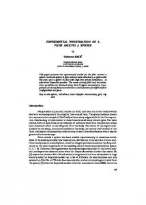
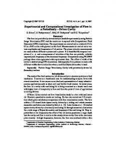
Figure 17 shows the two POD modes with the higher energy content in the symmetry plane of the SUV model. These two modes account for 31% of the total fluctuation energy. The first mode contains 17% and the second mode contains 14% of the total energy. The fluctuation energy of these modes is located primarily in the top shear layer. The main flow features of mode one are shown in Figure 17(a). There are two counter rotating vortices located at 525 mm and 600 mm respectively. Similarly, Figure 17(b) shows the spatial structure of mode 2. The main feature is a vortex located at 650 mm. These features suggest that the unsteady flow structure captured by these modes is a vortex shedding process of alternating sign vorticity similar to the vortex shedding process in the wake of a circular cylinder. The streamwise spacing of the vortices is approximately 75 mm or half the height of the SUV model. The two most energetic POD modes in the center horizontal plane of the wake are shown in Figure 18. The first and second mode energies are 12% and 8% of the total fluctuation energy, respectively. The spatial structure of the first mode is shown in Figure 18(a). This mode is antisymmetric relative to the plane of symmetry of the model, and features a strong lateral motion at approximately 650 mm. This is slightly downstream of the mean-flow recirculation region shown in Figure 14. Reconstruction of the velocity field associated with this mode suggests a lateral oscillation (flapping) of the entire wake. The spatial structure of the second mode is shown in Figure 18(b). This is a symmetric mode relative to the symmetry plane of the model. Reconstruction of the flow field associated with this mode shows a breathing oscillation of the recirculating flow region in the near wake.
(a)
(a)
(b) Figure 17. POD modes in the symmetry plane of the SUV model. (a) First mode; (b) Second mode.
(b) Figure 18. POD modes in the center horizontal plane of the SUV model wake. (a) First mode; (b) Second mode.
CONCLUSION
narrowing flow path, thus reducing pressure at both wheels.
This paper presents the results of an experimental investigation of the flow in the near wake of an SUV model. Results include the mean pressure distribution along the centerline and on the base of the model, the unsteady base pressure, PIV measurements of the flow in the near wake and POD analysis of the large scale turbulent flow structure in the near wake. The following conclusions can be derived from these results:
• The mean pressure coefficients measured on the base of the SUV shows lower values close to the bottom of the base and higher near the top of the base. The minimum value of the pressure coefficient is -0.23 at z ~ 25 mm which correspond to the location of the circulatory flow region in the near wake flow. The pressure coefficient at the upper edge of the base is approximately CP~ -0.1.
• The mean pressure distribution on the cabin of the SUV shows a stagnation region at the front grill and at the lower corner of the windshield, high speed and low pressure of the flow around the corners in front of the engine compartment and at the top of the windshield. The low pressure at the corners is followed by some pressure recovery on top of the engine hood and passenger compartment.
• The rms value of the pressure coefficient fluctuations measured at port B16 in the base of the SUV is about 1.72% of the dynamic pressure. The non-dimensional integral time is approximately 2.3 and the integral time scale is less than 15 ms.
• The underbody surface pressure distribution shows also the expected behavior. The local pressure is approximately the ambient static pressure except at the wheels where the flow accelerates due to the
• The spectrum of the pressure coefficient fluctuations in the base of the SUV shows a weak Strouhal peak approximately f* = 0.07 and large energy density at low frequencies possibly due to unsteadiness of the recirculating flow in the wind tunnel lab. This behavior indicates an unexpected sensitivity of the SUV flow field to very small amplitude fluctuations in the free
stream. The nature of this phenomenon is not well understood, although it can have significant practical consequences. • Mean velocity field measurements in the symmetry plane show a circulatory flow pattern near the bottom edge of the model. The length of this region is approximately 175 mm which is almost 1.2 times the width of the model. Also, another smaller circulatory flow pattern is found near the top shear layer. The underbody flow accelerates upward very rapidly towards the free stream flow in the near wake. The maximum reversed velocity in the recirculation region is approximately 0.35 times the free stream speed. These features of the flow are attributed to three dimensional effects introduced by the front body geometry. • In the symmetry plane there are two shear layers, one originating from top of the model and another one originating from the underbody flow. The rms value of the turbulence intensity is 23% of the free stream velocity in the top shear layer, and 12% of the free stream velocity in the underbody shear layer. The maximum shear correlation in the top shear layer is 0.0323 and is much smaller in the underbody shear layer (~0.01). • The main feature of the flow in the horizontal center plane is a relatively large symmetric recirculation region. The downstream extent of this region is about 175 mm which is almost 1.2 times the width of the model in good agreement with results in other flow geometries with blunt based models. The maximum upstream velocity in the wake is approximately 0.35 times the free stream speed which is in excellent agreement with the results in the symmetry plane. • The turbulence intensity in the side wall shear layers are somewhat lower than in the top shear layer (19%). The maximum shear correlation in the edge shear layers is significantly less than that in the top shear layer of the symmetry plane (0.02). • POD analysis of the PIV data show that the first two POD modes account for 31% and 20% of the fluctuation energy in the symmetry plane and the center horizontal plane, respectively. • These results suggest that the dominant unsteady structure in the symmetry plane is a vortex shedding process similar to the vortex shedding in the wake of a circular cylinder. • There are two dominant unsteady turbulent structures in the center horizontal plane: a lateral oscillation of the entire wake (flapping mode), and a breathing mode of the mean recirculation region.
ACKNOWLEDGMENTS This research was conducted at the Aerospace Engineering Department, University of Michigan, sponsored by General Motors Corporation. The work of A.M. Al-Garni was also supported by King Fahd
University of Petroleum and Minerals (KFUPM), Saudi Arabia.
REFERENCES 1
Al-Garni, A. M., Bernal, L. P., Khalighi, B., (2003) Experimental investigation of the near wake of a pickup truck, SAE Paper 2003-01-0651. 2 Al-Garni, A.M. Fundamental investigation of road vehicle aerodynamics, (2003) Ph.D. Thesis, Department of Aerospace Engineering, University of Michigan. 3 Lietz, R., Pien, W., Hands, D., and McGrew, J., (1999) Light truck aerodynamic simulations using a lattice gas based simulation technique, SAE Paper 1999-013756. 4 Bearman, P. W., Near wake flows behind twodimensional and three-dimensional bluff bodies, (1997) J. of Wind Eng. Ind. Aerodyn. 69-71, 33-54. 5 Balkanyi, S. R., Bernal, L. P., Khalighi, B., and Sumantran, V., (200) Dynamics of manipulated bluff body wakes, AIAA Paper 2000-2556, 2000. 6 Khalighi, B. Zang, S., Koromilas, C., Balkanyi, S., Bernal, L.P., Iaccarino, G. and Moin, P., (2001) Experimental and computational study of unsteady wake flow behind a body with a drag reduction device, SAE Paper 2001-01-1042. 7 Balkanyi, S., Bernal, L.P. and Khalighi, B., (2002) Analysis of the near wake of bluff bodies in ground proximity, ASME Paper 2002-32347. 8 Duell, E.G. and George, A.R., (1999) Experimental study of a ground vehicle body unsteady near wake, SAE Paper 1999-01-0812. 9 Deane, A. E., Kevrekidis, I.G., Karniadakis, G. E. and Orszag, S. A. (1991) Low-Dimensional Models for Complex Geometry Flows: Application to Grooved Channels and Circular Cylinders. Phys. Fluid, A 3 (10), 2337-2354. 10 Bernero, S. and Fiedler, H.E. (2000) Application of particle image velocimetry and proper orthogonal decomposition to the study of a jet in counterflow, Experiments in Fluids [Supl], S274-281. 11 Cipolla, K. M., Liakopoulos, A. and Rockwell, D. O. (1998) Quantitative Imaging in Proper Orthogonal Decomposition of Flow Past a Delta Wing. AIAA Journal, 36, No. 7, 1247-1255. 12 Lumely, J. L. (1967 )The Structure of Inhomogeneous turbulent flows. Atmospheric Turbulence and Radio Wave Propagation. Moscow, 167-178. 13 Sirovich, L. (1987) Turbulence and the Dynamics of Coherent Structures, Q. Appl. Math. 45, 561-590.