for the facts and the accuracy of the data presented herein. ... The goal was to limit the use of the service brakes on heavy duty vehicles by implementing a .... vehicle's cruise speed which is necessary for estimation of wheel slip. ...... generated versus engine RPM and curve fit the graph to garner a numerical model that.
CALIFORNIA PATH PROGRAM INSTITUTE OF TRANSPORTATION STUDIES UNIVERSITY OF CALIFORNIA, BERKELEY
Experimental Verification of Discretely Variable Compression Braking Control for Heavy Duty Vehicles Ardalan Vahidi, Anna G. Stefanopoulou, Phil Farias, Tsu Chin Tsao California PATH Research Report
UCB-ITS-PRR-2003-12
This work was performed as part of the California PATH Program of the University of California, in cooperation with the State of California Business, Transportation, and Housing Agency, Department of Transportation; and the United States Department of Transportation, Federal Highway Administration. The contents of this report reflect the views of the authors who are responsible for the facts and the accuracy of the data presented herein. The contents do not necessarily reflect the official views or policies of the State of California. This report does not constitute a standard, specification, or regulation. Report for Task Order 4234
March 2003 ISSN 1055-1425
CALIFORNIA PARTNERS FOR ADVANCED TRANSIT AND HIGHWAYS
Experimental Verification of Discretely Variable Compression Braking Control for Heavy Duty Vehicles Ardalan Vahidi
Phil Farias
Anna G. Stefanopoulou
Tsu Chin Tsao
University of Michigan
University of California, Los Angeles
TO 4234
Acknowledgments This work is supported in part by the California Partners for Advanced Transit and Highways (PATH) under TO 4234.
Experimental Verification of Discretely Variable Compression Braking Control for Heavy Duty Vehicles
Ardalan Vahidi Anna G. Stefanopoulou
Phil Farias Tsu Chin Tsao
Abstract In this report a recursive least square scheme with multiple forgetting factors is proposed for on-line estimation of road grade and vehicle mass. The estimated mass and grade can be used to robustify many automatic controllers in conventional or automated heavy-duty vehicles. We demonstrate with measured test data from the July 26-27, 2002 test dates in San Diego, CA, that the proposed scheme estimates mass within 5% of its actual value and tracks grade with good accuracy. The experimental setup, signals, their source and their accuracy are discussed. Issues like lack of persistent excitations in certain parts of the run or difficulties of parameter tracking during gear shift are explained and suggestions to bypass these problems are made. Finally, the steps taken for developing the compression brake map, transmission map and tuning a controller for coordinated use of service and compression brake are explained. Using the data from the July 26-27, 2002 test dates in San Diego, CA, we show in simulation that the inclusion of the splitting torques scheme resulted in a service brake use decrease of 90 percent.
Keywords Advanced Vehicle Control Systems Parameter Estimation
Speed Control System Identification
Executive Summary This report describes vehicle parameter estimation, system identification and tuning of a controller for coordination of compression and service brakes based on the data acquired during open-loop road tests. In the first part of the report, development and verification of a parameter estimation scheme for online estimation of vehicle’s mass and road grade are described. First a survey on related literature and patents is provided. We then propose a recursive least square scheme with forgetting for estimation of mass and time-varying grade. We demonstrate, both with simulated and test data, that the proposed scheme estimates mass and grade with good accuracy provided persistent excitations. The experimental setups, signals, their source and their accuracy are discussed. The real life issues like lack of persistent excitations in certain parts of the run or difficulties of parameter tracking during gear shift are explained and suggestions to bypass these problems are made. In the second part of the report, the steps taken for developing the compression brake map, transmission map and tuning a controller for coordinated use of service and compression brake are explained. The goal was to limit the use of the service brakes on heavy duty vehicles by implementing a splitting torque scheme that uses the compression brake in conjunction with the service brake to maintain a desired speed. With data acquired from the July 26-27, 2002 test dates in San Diego, CA we were able to develop a mathematical model the compression brake that gave the negative braking torque available as a function of the current engine speed. We constructed a transmission map of the vehicle that we used to approximate its shifting schedule and both were added to the vehicle dynamics model that was identified in part one. We then tuned a fixed gain PI controller for velocity tracking and came up with a braking algorithm that decided when and how to use the compression brake. These were cascaded with the vehicle model to give our closed loop system for the vehicle that tracked a reference velocity as it went through the available road profile. In this simulation, the inclusion of the splitting torques scheme resulted in a service brake use decrease of 90 percent.
Contents 1 Parameter Estimation 1.1 Introduction . . . . . . . . . . . . . . . . . . . . . . . . . . . . . . . . . . . . . . . . 1.2 Mass and Grade Estimation: State of the Art . . . . . . . . . . . . . . . . . . . . . 1.3 Formulation of the Estimation Problem . . . . . . . . . . . . . . . . . . . . . . . . 1.3.1 Longitudinal Dynamics Equation . . . . . . . . . . . . . . . . . . . . . . . . 1.3.2 Recursive Least Square Estimation . . . . . . . . . . . . . . . . . . . . . . . 1.3.3 Recursive Least Square Estimation with Forgetting . . . . . . . . . . . . . . 1.3.4 A Recursive Least Square Scheme with Multiple Forgetting . . . . . . . . . 1.4 Simulation Analysis of Single and Multiple Forgetting Methods . . . . . . . . . . . 1.4.1 Numerical Problems in Presence of Signal Noise . . . . . . . . . . . . . . . 1.5 Experimental Setups: Open-Loop Experiments . . . . . . . . . . . . . . . . . . . . 1.6 Experimental System Identification . . . . . . . . . . . . . . . . . . . . . . . . . . . 1.6.1 Measured Signals . . . . . . . . . . . . . . . . . . . . . . . . . . . . . . . . . 1.6.2 Determining Unknown Parameters . . . . . . . . . . . . . . . . . . . . . . . 1.7 Performance of the Estimator with Experimental Data . . . . . . . . . . . . . . . . 1.7.1 Estimation in Normal Cruise: No Gearshift . . . . . . . . . . . . . . . . . . 1.7.2 Estimation Results During Gearshift: Problem and Recommended Solution 1.7.3 Sensitivity Analysis . . . . . . . . . . . . . . . . . . . . . . . . . . . . . . . 1.8 Conclusions and Discussions . . . . . . . . . . . . . . . . . . . . . . . . . . . . . . .
. . . . . . . . . . . . . . . . . .
. . . . . . . . . . . . . . . . . .
. . . . . . . . . . . . . . . . . .
. . . . . . . . . . . . . . . . . .
4 4 5 5 5 6 7 9 11 16 16 17 17 18 19 20 21 23 23
2 Compression Brake Characterization 2.1 Introduction . . . . . . . . . . . . . . . . . . . . . . . . . . . 2.2 Compression Brake Model . . . . . . . . . . . . . . . . . . . 2.2.1 Model Validation Test . . . . . . . . . . . . . . . . . 2.3 Transmission Model and Map . . . . . . . . . . . . . . . . . 2.4 Integrated Friction and Compression Brake Control Scheme 2.4.1 Brake Control Algorithm . . . . . . . . . . . . . . . 2.4.2 PI Control Tuning . . . . . . . . . . . . . . . . . . . 2.4.3 Vehicle Dynamics Model . . . . . . . . . . . . . . . . 2.5 Conclusions . . . . . . . . . . . . . . . . . . . . . . . . . . . 2.5.1 Future Work . . . . . . . . . . . . . . . . . . . . . .
. . . . . . . . . .
. . . . . . . . . .
. . . . . . . . . .
. . . . . . . . . .
26 26 26 27 28 30 31 32 33 36 39
3 Appendix
. . . . . . . . . .
. . . . . . . . . .
. . . . . . . . . .
. . . . . . . . . .
. . . . . . . . . .
. . . . . . . . . .
. . . . . . . . . .
. . . . . . . . . .
. . . . . . . . . .
. . . . . . . . . .
. . . . . . . . . .
. . . . . . . . . .
. . . . . . . . . .
40
1
List of Figures 1.1 1.2 1.3 1.4 1.5 1.6 1.7 1.8 1.9
1.10 1.11
1.12
1.13 2.1 2.2 2.3 2.4 2.5 2.6 2.7
Estimation of mass and grade using RLS with a single forgetting factor of 0.8 when grade is piecewise constant. . . . . . . . . . . . . . . . . . . . . . . . . . . . . . . . . . . . . . . . Estimation of mass and grade using RLS with a single forgetting factor of 0.9 when grade variations are sinusoidal. . . . . . . . . . . . . . . . . . . . . . . . . . . . . . . . . . . . . . Estimation of mass and grade using RLS with multiple forgetting factors of 0.8 and 1 respectively for grade and mass. . . . . . . . . . . . . . . . . . . . . . . . . . . . . . . . . . Estimation of mass and grade using RLS with multiple forgetting factors of 0.5 and 1 respectively for grade and mass. . . . . . . . . . . . . . . . . . . . . . . . . . . . . . . . . . Estimation of mass and grade using RLS with vector-type forgetting. Forgetting factor of 0.98 was used for both mass and grade. . . . . . . . . . . . . . . . . . . . . . . . . . . . . Estimation of mass and grade using our proposed scheme. Forgetting factor of 0.98 was used for both mass and grade. . . . . . . . . . . . . . . . . . . . . . . . . . . . . . . . . . . Digitized road elevation and grade. . . . . . . . . . . . . . . . . . . . . . . . . . . . . . . . Comparison of the model and real longitudinal dynamics. . . . . . . . . . . . . . . . . . . Estimator’s performance during normal cruise when the gear is constant. Forgetting factors for mass and grade are 0.95 and 0.4 respectively. RMS error in mass is 350 kg and RMS grade error is 0.2 degrees. . . . . . . . . . . . . . . . . . . . . . . . . . . . . . . . . . . . . The performance during a cycle of pulsing the throttle . . . . . . . . . . . . . . . . . . . . Estimator’s performance when it is always on. Forgetting factors for mass and grade are 0.99 and 0.4 respectively. The RMS errors in mass and grade are 210 kg and 0.8 degrees respectively. . . . . . . . . . . . . . . . . . . . . . . . . . . . . . . . . . . . . . . . . . . . . Estimator’s performance when it is turned off during shift. Forgetting factors for mass and grade are 0.99 and 0.4 respectively. The RMS errors in mass and grade are 160 kg and 0.23 degrees respectively. . . . . . . . . . . . . . . . . . . . . . . . . . . . . . . . . . . . . . Sensitivity of the estimates with respect to drag coefficient and rolling resistance. Forgetting factors for mass and grade are 0.95 and 0.4 respectively. . . . . . . . . . . . . . . . . Compression brake map depicting the amount of negative torque available by the compression brake in high or low mode for a given engine speed. . . . . . . . . . . . . . . . . . . . Compression brake model validation. The model was tested to see how well it predicted the compression brake outputs for various test runs . . . . . . . . . . . . . . . . . . . . . . Transmission map that is based on data acquired from test runs. The gear number is plotted as a function of accelerator pedal position and output shaft speed. . . . . . . . . . Comparison of the predicted gear of the vehicle as determined by the transmission shifting model and the actual gear the vehicle was in. . . . . . . . . . . . . . . . . . . . . . . . . . Comparison of the predicted gear of the vehicle as determined by the transmission shifting model and the actual gear the vehicle was in. . . . . . . . . . . . . . . . . . . . . . . . . . An example of how the braking algorithm would vacillate between service brake usage and compression brake usage resulting in the simulations stalling . . . . . . . . . . . . . . . . . Vehicle Dynamics Model . . . . . . . . . . . . . . . . . . . . . . . . . . . . . . . . . . . . .
2
12 13 13 14 15 15 18 19
20 21
22
22 23 27 28 29 29 30 32 35
2.8 2.9 2.10 2.11 2.12
Complete Closed Loop System . . . . . . . . . . . . . . . . . . . . . Velocity tracking through the grade for models with and without the Integrated values of braking usage through the grade . . . . . . . . Braking distribution for the model with transmission map. . . . . . . Braking distribution for the model without transmission map. . . . .
3
. . . . . . . . . . . transmission map . . . . . . . . . . . . . . . . . . . . . . . . . . . . . . . . .
. . . . .
35 36 37 38 38
Chapter 1
Parameter Estimation 1.1
Introduction
The linear parameter estimation problem arises in a broad class of scientific disciplines. In systems and control specifically, it is widely used in open-loop applications like plant modelling and in closed loop for applications like adaptive control. It can be viewed also in the context of system identification where the key steps are selection of the model, experimental design, parameter estimation and validation. Parameter estimation techniques can be used in direct system identification before the control design process. An online estimation scheme appears explicitly as a component of self-tuning regulator. Also in adaptive control scheme an online estimation method occurs implicitly [3]. It tracks time-varying parameters or estimates external disturbances to the system. In vehicle control, many control decisions can be improved if the unknown parameters of the vehicle model can be estimated. Weight of the vehicle, coefficient of rolling resistance, and drag coefficient are among these unknown parameters. Road grade is a major source of external loading which is normally unknown. A transmission control logic can use grade estimates for improved gear change scheduling and to avoid “gear hunting”. An anti-lock brake controller relies on an estimate of mass and road grade for calculating vehicle’s cruise speed which is necessary for estimation of wheel slip. In longitudinal control of platoons of vehicles, precise spacing is necessary for ensuring the stability of the string of vehicles and therefore reliable estimation of external loads and vehicle parameters is important. For heavy vehicles mass and grade are even more important. The mass of a heavy duty vehicle can vary as much as %400 depending on the load it carries. Mild grades for passenger vehicles, are serious loadings for heavy vehicles. Therefore estimation of mass and grade is particularly critical for heavy duty vehicles. Online estimation schemes which can estimate mass, grade or both have been investigated before, but the problem remains open as each of the existing algorithms has its own shortcomings. In this chapter after a review of the existing schemes for mass and grade estimation we investigate implementation of a recursive least square (RLS) method for simultaneous online mass and grade estimation. We briefly cover the recursive least square scheme for time varying parameters and review some key papers that address the subject. The difficulty of the popular RLS with single forgetting is discussed next. For estimation of multiple parameters which vary with different rates, RLS with vector-type forgetting is previously proposed in a few papers. We analyze this approach and propose an extension with intuitive appeal. We demonstrate, both with simulated and test data, that incorporating two distinct forgetting factors is effective in resolving the difficulties in estimating mass and time-varying grade. The experimental setups and particular issues with experimental data is also discussed.
4
1.2
Mass and Grade Estimation: State of the Art
Vehicle parameter estimation, specifically mass and grade estimation for heavy vehicles, has been visited by researchers in industry and academia. The proposed schemes can in general be classified in two categories: sensor-based and model-based methods. In sensor based methods some type of extra sensor is used on the vehicle to facilitate estimation of one or more parameters. Model-based schemes use a model of the vehicle and only the data that is available through the CanBus for estimation. Since longitudinal dynamics of the vehicle depends on both mass and grade, knowing one will facilitate estimation of the other. Therefore some suggest estimating the grade which is in general time varying with some type of sensor and then estimating the mass with conventional parameter-adaptive algorithms [14],[29]. Bae et al. [4] use GPS readings to obtain road elevation and calculate the grade using the measured elevations. With the grade known, they estimate the mass with a simple least square method based on the longitudinal dynamics equation. In [21] using an on-board accelerometer is proposed for grade estimation. The mass is estimated based on a good approximations of the grade. The problem however is the cost of additional sensors and the increased effort necessary to process the data measured by these sensors. For example accelerometer-based schemes are highly susceptible to noise and in many occasions the recorded data may not be useful. One approach [12] which has been patented and has been used in industry is estimation of mass based on the velocity drop during a gearshift. The idea is that since the gearshift period is short, the road load can be rendered constant. The change in velocity before and during gearshift can be used to calculate an estimate for the mass based on the longitudinal dynamics equation. However based on a fair amount of trial, we observed that the velocity drop is normally minor during a gearshift and this limits the accuracy of the method. Besides this approach does not address estimation of the grade. Within an adaptive control scheme Druzhinina et al. [10] provide simultaneous mass and road grade estimation without additional sensors. They demonstrate convergence in estimates for constant mass and piecewise constant grade. This method is an indirect estimation method since estimation is achieved in closed-loop and as a by-product of a control scheme. In general the grade is not piecewise constant and it can vary linearly during slope transitions. Moreover many times estimates independent of a controller are required. In other words a direct estimation scheme is more appealing. In the rest of this chapter we will investigate a direct approach for simultaneous estimation of mass and time-varying grade. Throughout the derivations and analysis we will point to the advantages and difficulties of the scheme.
1.3
Formulation of the Estimation Problem
Our estimation approach is a model based approach. That is, we rely on a physical model of vehicle’s longitudinal dynamics and use this model and the data that is recorded from the vehicle’s CanBus for estimating mass and grade and possibly other unknown parameters which affect vehicle’s longitudinal motion. Therefore we first formulate the vehicle longitudinal dynamics equation.
1.3.1
Longitudinal Dynamics Equation
A vehicle’s acceleration is a result of combination of engine and braking torques and the road loads on the vehicle. When the torque convertor and the driveline are fully engaged we can assume that all the torque from the engine is passed to the wheel. Further assuming that there is no wheel slip, which is a good assumption for most part of the motion, the longitudinal dynamics can be presented in the following simple but accurate form: Te − Je ω˙ − Ff b − Faero − Fgrade (1.1) M v˙ = rg In this equation M is the total mass of the vehicle, v is the cruise velocity and ω is rotational engine speed. Te is the engine torque at the flywheel. If engine is in fuelling mode the torque is positive and if it 5
is in the compression braking mode the torque is negative. If the transmission and the torque convertor are fully engaged then most of the torque is passed to the wheels as assumed in the above equation. To model the possible torque losses, engine torque can be scaled down by a coefficient of efficiency. Je is the powertrain inertia and therefore the term Je ω˙ represents the portion of torque spent on rotating the powertrain. Ff b is the generated friction brake (service brake) force at the wheels. The force due to aerodynamic resistance is given by 1 Faero = Cd ρAv 2 2 where Cd is the drag coefficient, ρ is air density and A is frontal area of the vehicle. Fgrade describes the combined force due to road grade (β) and the rolling resistance of the road (µ). It is given by Fgrade = M g(−µ cos β − sin β), where g is gravity. Here β = 0 corresponds to no inclination, β > 0 corresponds to uphill grade and β < 0 represents downhill. We are interested in using this equation along with the data that is obtained from vehicle’s CanBus for online estimation of mass and grade. Eq. (1.1) can be rearranged so that mass and grade are separated into two terms: Te − Je ω˙ g 1 v˙ = ( (1.2) − Ff b − Faero ) − sin(β + βµ ) rg M cos(βµ ) where tan(βµ ) = µ. We can rewrite the equation in the following linear parametric form, y = φT θ, φ = [φ1 φ2 ]T θ = [θ1 θ2 ]T Where θ = [θ1 , θ2 ]T = [
(1.3)
1 , sin(β + βµ )]T M
is the parameter of the model, which we try to estimate and y = v, ˙ φ1 =
Te − Je ω˙ g − Ff b − Faero , φ2 = − rg cos(βµ )
can be calculated based on measured signals and known variables. Had the parameters θ1 and θ2 been constant, a simple recursive algorithm, like recursive least squares, could have been used for estimation. However while θ1 which depends only on mass is constant, the parameter θ2 is in general time-varying. Tracking time-varying parameters needs provisions that we will discuss next. In the next sections we first discuss the recursive least square problem and subsequently the concept of forgetting for tracking time varying parameters.
1.3.2
Recursive Least Square Estimation
At the end of the eighteenth century Karl Freidrich Gauss proposed the simple and brilliant method of least squares and used this principle to determine the orbits of planets. He stated that the unknown parameters of a model should be chosen in such a way that the sum of the squares of the difference between the actually observed and the computed values, weighted by their degree of precision, is a minimum [3]. For a linear system that translates into finding the parameter(s) that minimizes the following “lossfunction”, k ¢2 1 X¡ (1.4) y(i) − φT (i)θ V (θ, t) = 2 i=1 6
Solving for the minimizing parameters we get the closed form solution as follows: θˆ =
à k X
!−1 Ã φ(i)φT (i)
i=1
k X
! φ(i)y(i)
(1.5)
i=1
Most of the time we are interested in real-time parameter estimation. Therefore it is computationally more efficient if we update the estimates in (1.5) recursively as new data becomes available online. The recursive form is given by: ³ ´ ˆ ˆ − 1) + L(k) y(k) − φT (k)θ(k ˆ − 1) θ(k) = θ(k (1.6) where and
¡ ¢−1 L(k) = P (k)φ(k) = P (k − 1)φ(k) 1 + φT (k)P (k − 1)φ(k)
(1.7)
¡ ¢ P (k) = I − L(k)φT (k) P (k − 1)
(1.8)
P (K) is normally referred to as the covariance matrix. More detailed derivation can be found in books on parameter estimation such as [3]. For convergence proof see for example the book by Johnson [15]. Eq. (1.6) updates the estimates at each step based on the error between the model output and the predicted output. The structure is similar to most recursive estimation schemes. In general most have similar parameter update structure and the only difference is the update gain L(k). The scheme can be viewed as some type of filter that averages the data to come up with optimal estimates. Averaging is a good strategy if parameters of the model are constant in nature. However many times the parameters that we are estimating are time-varying and we are interested to keep track of this variations. Next section will discuss the generalized RLS for time-varying parameters.
1.3.3
Recursive Least Square Estimation with Forgetting
If the change in the parameters of a system is abrupt, periodic resetting of the estimation scheme can potentially capture the new values of the parameters. However if the parameters vary continuously but slowly a different heuristic but effective approach is popular. That is the concept of forgetting in which older data is gradually discarded in favor of more recent information. In least square, forgetting can be viewed as giving less weight to older data and more weight to recent data. The “loss-function” is then defined as follows: k ¢2 1 X k−i ¡ V (θ, t) = λ y(i) − φT (i)θ(k) (1.9) 2 i=1 where λ is a positive parameter smaller than 1 and is called the forgetting factor. It operates as a weight which diminishes for the more remote data. The scheme is known as least-square with exponential forgetting and θ can be calculated recursively using the same update equation (1.6) but with L(k) and P (k) derived as follows: ¡ ¢−1 L(k) = P (k − 1)φ(k) λ + φT (k)P (k − 1)φ(k) and
(1.10)
¡ ¢ 1 P (k) = I − L(k)φT (k) P (k − 1) . (1.11) λ The main difference with the classical least square method is how the covariance matrix P (k) is updated. In the classical RLS the covariance vanishes to zero with time, losing its capability to keep track of changes in the parameter. In (1.11) however, the covariance matrix is divided by λ < 1 at each update. This slows down fading out of the covariance matrix. The exponential convergence of the above scheme is shown in some textbooks and research papers (See e.g. the proof provided in [6] or [15]) for the case of unknown
7
but ”constant” invariant case. In general exponential convergence in the constant case implies certain degree of tracking capability in the time varying case [7]. However rigorous mathematical analysis of tracking capabilities of an estimator when the parameters are time-varying are rare in literature and many properties are demonstrated through simulation results. Campi [7] provides some rigorous mathematical arguments that if the covariance matrix of the estimator is kept bounded the tracking error will remain bounded. Ljung and Gunnarsson present a survey of algorithms for tracking time-varying systems in [18]. The RLS with forgetting has been widely used in estimation and tracking of time-varying parameters in various fields of engineering. However when excitations to the system are poor this scheme can lead to the covariance “wind-up” problem. During poor excitations old information is continuously forgotten while there is very little new dynamic information coming in. This might lead to the exponential growth of the covariance matrix and as a result the estimator becomes extremely sensitive and therefore susceptible to numerical and computational errors [11]. This problem has been investigated by many researchers in the field and several solutions, mostly ad hoc, have been proposed to avoid covariance “wind-up”. The idea of most of these schemes is to limit the growth of covariance matrix for example by introducing an upper bound. A popular scheme is proposed by Fortescue et al. [11] in which a time-varying forgetting factor is used. During low excitations, the forgetting factor is closer to unity to enhance the performance of the estimator. In another approach, Sripada and Fisher [27] propose an on/off method along with a time-varying forgetting factor for improved performance. The concept of resetting the covariance matrix during low excitations has been also investigated in [26]. Both papers provide good discussions about behavior of the system during low excitations. Kulhavy and Zarrop discuss the concept of forgetting from a more general perspective in [17]. One other popular refinement to the RLS with forgetting scheme is the concept of “directional forgetting” for reducing the possibility of the estimator windup when the incoming information is non-uniformly distributed over all parameters. The idea is that if a recursive forgetting method is being used, the information related to non-excited directions will gradually be lost. This results in unlimited growth of some of the elements of the covariance matrix and can lead to large estimation errors. Implementation of the concept of directional forgetting is again ad hoc and is reflected in updating the covariance matrix, P (k). That is, if the incoming information is not uniformly distributed in the parameter space the proposed schemes perform a selective amplification of the covariance matrix. Hagglund [13] and Kulhavy [16] have developed one of the early versions of this algorithm. Bittani et al. discuss the convergence of RLS with directional forgetting in [5]. Cao and Schwartz [8] explain some of the limitations of the earlier directional forgetting scheme and propose an improved directional forgetting approach. The estimator wind-up can also occur if we are estimating multiple parameters that each (or some) vary with a different rate. This scenario is of particular interest in the problem of mass and grade estimation where mass is constant and grade is time-varying. It will be shown by simulation later in this chapter that the single forgetting algorithm is not be able to track parameter with different variation rates. Therefore it is desirable to assign different forgetting factors to different parameters. This problem is somehow similar but not equivalent to the case when excitations are non-uniform in the parameter space. In the author’s opinion even when all the modes are uniformly excited, different rate of variations of parameters can cause trouble in estimation. An ad hoc remedy to this problem has been suggested in a few publications and is known as vector-type forgetting [24], [25] or selective forgetting [22]. The idea is again implemented in the update of covariance matrix. Instead of dividing all elements by a single λ, P is scaled by a diagonal matrix of forgetting factors: ¡ ¢ (1.12) P (k) = Λ−1 I − L(k)φT (k) P (k − 1)Λ−1 where Λ = diag[λ1 , λ2 , . . . , λn ] in an n-parameter estimation and λi is the forgetting factor reflecting the rate of the change of the ith parameter. The author has found this method an effective way of keeping track of the parameters that change with different rates. The few examples of application of this scheme, to the best knowledge of the
8
author, can be found in [30], and [20]. Yoshitani and Hasegawa [30] have used a vector-type forgetting scheme for parameter estimation in control of strip temperature for the heating furnace. For a self-tuning cruise control Oda et al. [20] propose using vector-type forgetting for detecting step changes in the parameters of a transfer function. Like most other modifications to RLS with forgetting, mathematical proofs for tracking capabilities of the method, to the best knowledge of the author, do not exist. However a proof for convergence to constant parameter values can be found in [23]. In [23] a general class of RLS with forgetting is formulated and vector type forgetting is also included as a special case. Exponential convergence to constant parameter values is proved for this general class of estimators. Before employing the vector-type forgetting, and to remedy the problems associated with various rates of variations, the authors had formulated a multiple forgetting method which has similarities to and differences from the above-mentioned schemes. It has shown very good convergence and tracking capabilities in simulation and experiments and the way it is formulated makes an intuitive sense. Since it provides some motivation on the concept of multiple forgetting, we discuss the formulation and the structure of the problem in the next section.
1.3.4
A Recursive Least Square Scheme with Multiple Forgetting
When working on the particular mass and grade estimation problem, the author noticed that the difficulties in RLS with single forgetting stem from the following facts: 1. In the standard method it is assumed that the parameters vary with similar rates. 2. In the formulation of the loss-function defined in (1.9) and subsequently the resulting recursive scheme, the errors due to all parameters are lumped into a single scalar term. So the algorithm has no way to realize if the error is due to one or more parameters. As a result if there is drift in a single parameter, corrections of the same order will be applied to all parameters which results in over-shoot or undershoot in the estimates. If the drift continues for sometime it might cause poor overall performance of the estimator or even the so-called estimator “wind-up” or “blow-up”. It is true that we are fundamentally restricted by the fact that the number of existing equations is less than number of parameters which we are estimating, but in a tracking problem we can use our past estimation results more wisely by introducing some kind of “decomposition” in the error due to different parameters. Therefore, our intention is to“separate” the error due to each parameter and subsequently apply a suitable forgetting factor for each. Without loss of generality and for more simple demonstration, we shall assume that there are only two parameters to estimate. We define: V (θˆ1 (k), θˆ2 (k), k) =
1 2
³ ´2 λk−i y(i) − φ1 (i)θˆ1 (k) − φ2 (i)θ2 (i) + 1 ³ ´2 Pk k−i 1 y(i) − φ1 (i)θ1 (i) − φ2 (i)θˆ2 (k) i=1 λ2 2 Pk
i=1
(1.13)
With this definition for the loss function the first term on the right hand side of (1.13) represents only the error of the step k due to first parameter estimate, θˆ1 (k) and the second term corresponds to the second parameter estimate, θˆ2 (k). Now each of these errors can be discounted by an exclusive forgetting factor. Here λ1 and λ2 are forgetting factors for first and second parameters respectively. Incorporating multiple forgetting factors provides more degrees of freedom for tuning the estimator, and as a result, parameters with different rates of variation could possibly be tracked more accurately. The optimal estimates are those that minimize the loss function and are obtained as follows: k ³ ´ X ∂V ˆ =0⇒ λk−i (−φ (i)) y(i) − φ (i) θ (k) − φ (i)θ (i) =0 1 1 1 2 2 1 ∂ θˆ1 (k) i=1
9
(1.14)
Rearranging (1.14), θˆ1 (k) is found to be: Ã θˆ1 (k) =
k X
!−1 Ã 2 λk−i 1 φ1 (i)
k X
i=1
! λk−i 1
(y(i) − φ2 (i)θ2 (i))
(1.15)
i=1
Similarly θˆ2 (k) will be: Ã θˆ2 (k) =
k X
!−1 Ã 2 λk−i 2 φ2 (i)
k X
! λk−i 2
(y(i) − φ1 (i)θ1 (i))
(1.16)
i=1
i=1
For real time estimation a recursive form is required. Using the analogy that is available between (1.15), (1.16) and the classical form (1.5), the recursive form can be readily deduced: ³ ´ θˆ1 (k) = θˆ1 (k − 1) + L1 (k) y(k) − φ1 (k)θˆ1 (k − 1) − φ2 (k)θ2 (k) (1.17) where
¡ ¢−1 L1 (k) = P1 (k − 1)φ1 (k) λ1 + φT1 (k)P1 (k − 1)φ1 (k) ¡ ¢ 1 P1 (k) = I − L1 (k)φT1 (k) P1 (k − 1) . λ1
and similarly,
³ ´ θˆ2 (k) = θˆ2 (k − 1) + L2 (k) y(k) − φ1 (k)θ1 (k) − φ2 (k)θˆ2 (k − 1)
where
(1.18)
¡ ¢−1 L2 (k) = P2 (k − 1)φ2 (k) λ2 + φT2 (k)P2 (k − 1)φ2 (k) ¢ ¡ 1 P2 (k) = I − L2 (k)φT2 (k) P2 (k − 1) . λ2
In the two aforementioned equations θˆ1 (k), θˆ2 (k), θ1 (k), and θ2 (k) are the unknowns. As is customary in similar problems, θ1 (k), and θ2 (k) can be replaced with their estimates, θˆ1 (k) and θˆ2 (k).1 Upon substitution for θ1 (k) and θ2 (k) and rearranging (1.17) and (1.18) we obtain: ³ ´ θˆ1 (k) + L1 (k)φ2 (k)θˆ2 (k) = θˆ1 (k − 1) + L1 (k) y(k) − φ1 (k)θˆ1 (k − 1) (1.19) ³ ´ L2 (k)φ1 (k)θˆ1 (k) + θˆ2 (k) = θˆ2 (k − 1) + L2 (k) y(k) − φ2 (k)θˆ2 (k − 1)
(1.20)
For which the solution is, ·
θˆ1 (k) θˆ2 (k)
¸
· =
1 L1 (k)φ2 (k) L2 (k)φ1 (k) 1
The determinant of the matrix
1 Note
·
¸−1
³ ´ θˆ1 (k − 1) + L1 (k) y(k) − φ1 (k)θˆ1 (k − 1) ³ ´ θˆ2 (k − 1) + L2 (k) y(k) − φ2 (k)θˆ2 (k − 1)
1 L2 (k)φ1 (k)
L1 (k)φ2 (k) 1
¸
that we could have introduced the loss function as follows instead:
V (θˆ1 , θˆ2 , k) =
k k �2 �2 1 X k−i � 1 X k−i � y(i) − φ1 (i)θˆ1 (k) − φ2 (i)θˆ2 (i) + y(i) − φ1 (i)θˆ1 (i) − φ2 (i)θˆ2 (k) λ1 λ2 2 i=1 2 i=1
.
10
(1.21)
is always nonzero and therefore the inverse always exists. With some more mathematical manipulations (1.21) can be written in the form of (1.6): ³ ´ ˆ ˆ − 1) + Lnew (k) y(k) − φT (k)θ(k ˆ − 1) θ(k) = θ(k (1.22) where Lnew (k) is defined as follows: Lnew (k) =
"
1 1+
P1 (k−1)φ1 (k)2 λ1
+
P2 (k−1)φ2 (k)2 λ2
P1 (k−1)φ1 (k) λ1 P2 (k−1)φ2 (k) λ2
# (1.23)
The proposed method incorporates different forgetting factors for each parameter. To this end, it does what the vector-type forgetting method does. Eq. (1.22) is similar in form to the standard update of (1.6). However the gains of the standard and the proposed form are different. Specifically the former has a crossterm P12 (k − 1), while the latter does not. In other words the covariance matrix of the proposed method is diagonal. This will result in update of the two parameters proportional to P1 (k) and P2 (k). In short, introduction of the loss-function (1.13) with decomposed errors and different forgetting factors for each have two distinct implications: 1) Parameters are updated with different forgetting factors. That is done by scaling the covariances by different forgettings. This is more or less what is done in the RLS with vector-type forgetting as well. However this approach is based on minimization of a loss-function. 2) It decouples the updating step of the covariance of different parameters. This is different from standard RLS or RLS with vector-type forgetting. The author believes that when the parameters are independent of each other this makes an intuitive sense. The above equations can be generalized to cases with more than two parameters. This can be done with tedious recalculation of the gains or by just inferring from the two-parameter case. The proposed scheme has the added advantage that it reduces the computational burden of inverting the covariance matrix which its size grows with the number of unknown parameters. This scheme did well in both simulation and experiments of mass-grade estimation. The performance is very similar to the RLS with vector forgetting when similar forgetting factors are used. However if the value of the forgetting factors are picked in a way that mismatches real rate of variations of the parameters, it was observed that RLS with vector forgetting sometimes winds up. In such a situation the estimator was excessively sensitive to noise. On the other hand, the proposed scheme always behaved well and mismatch between forgetting and true rate of variations did not cause the windup behavior. In the following section we carefully select the forgetting factors of the vector-type forgetting RLS so that the response compares favorably with the decoupled vector forgetting that we proposed.
1.4
Simulation Analysis of Single and Multiple Forgetting Methods
We first use simulated data to test a recursive scheme for estimation of mass and grade. The simulated data was generated using the vehicle dynamics model given in (1.2) and by assuming different road grade profiles and feasible mass and parameters for a heavy duty vehicle. A feasible fuelling pattern was chosen. Variation of fuelling is important in exciting all modes of the system and consequently allow better estimation results. Therefore in generating the fuelling command this was taken into account. The engine torque was then readily calculated based on fuelling rate and engine speed by using the engine torque map. At this stage we assumed that no gear change occurs during the estimation process. In the next sections, we will discuss the issue of gear change and explain how it can be incorporated in experimental estimation. We use a recursive least square scheme for estimating and tracking the parameters. For initialization, we employ a direct least square on a batch of first few seconds of data. This initializes the estimates and the P matrix.
11
5
Grade [deg]
Estimated Grade Actual Grade
0
−5
0
10
20
30
40
50
Time, s
60
70
80
90
100
4
3
x 10
Estimated Mass Actual Mass
Mass [kg]
2.5 2
1.5 1
0.5 0
0
10
20
30
40
50
Time,s
60
70
80
90
100
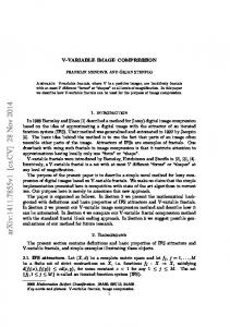
Figure 1.1: Estimation of mass and grade using RLS with a single forgetting factor of 0.8 when grade is piecewise constant. First we used the RLS with single forgetting for estimation of mass and tracking grade. For the reasons explained in previous sections of this chapter the results were not promising at all. First we considered a constant mass and step changes in grade. The data that we used was clean from any noise. Figure 1.1 shows the estimation results. We observe big overshoots or undershoots in both mass and grade estimates during step changes in grade or fuelling. Nevertheless we see a relatively fast convergence back to the real parameter values after the deviations. That is in line with the proofs of convergence of RLS with or without forgetting to constant parameter values. To this end, despite the local misbehavior we can still get some estimates for both parameters. The main difficulty of the approach appears when one of the parameters, here the grade, starts varying continuously (as opposed to staying piecewise constant). The algorithm shows very poor tracking performance in such a scenario. Figure 1.2 shows the estimator performance when grade variations are sinusoidal. The well-known phenomenon of estimator “blow-up” or “wind-up” can be seen during grade changes. Errors in both mass and grade estimates become very large. The estimates converge back to the real values only when the grade becomes constant. Here a forgetting factor of 0.9 is chosen. We noticed that reducing the forgetting factor will only worsen the problem. When noise is introduced in the data, the performance is sacrificed even more. As explained in the formulation of the problem, the reason for the poor performance is that when an error is detected the estimates for both parameters are updated without differentiating between the ones that vary faster and those that do not vary as often or are constant. This causes overshoot/undershoot in the estimates. If one parameter continues drifting, the estimation errors add up to result in what was seen in the previous figures. We carried out simulations using RLS with multiple forgetting factors and showed that this scheme can resolve the problems encountered with single forgetting. Figure 1.3 shows the performance of the estimator when grade goes through step-changes. In this example forgetting factors of 0.8 and 1.0 are chosen for grade and mass respectively. Unlike estimation with single forgetting, the estimation is very smooth and the estimates converge much faster during step changes. Because a forgetting factor of 1.0 is chosen for mass, the mass estimates are not as sensitive to changes in grade. We also tried sinusoidal variations in grade. The results are shown in Figure 1.4. The grade is tracked
12
10
Grade [deg]
Estimated Grade Actual Grade 5
0
−5
−10
0
10
20
30
40
50
60
70
80
90
100
4
10
x 10
Estimated Mass Actual Mass
Mass [kg]
8 6 4 2 0 0
10
20
30
40
50
Time,s
60
70
80
90
100
Time, s
Figure 1.2: Estimation of mass and grade using RLS with a single forgetting factor of 0.9 when grade variations are sinusoidal.
3 Estimated Grade Actual Grade
Grade [deg]
2 1 0
−1
Time, s
−2 −3
0
10
20
30
40
50
60
70
80
90
100
4
2.5
x 10
Estimated Mass Actual Mass
Mass [kg]
2 1.5 1
0.5 0
0
10
20
30
40
50
Time,s
60
70
80
90
100
Figure 1.3: Estimation of mass and grade using RLS with multiple forgetting factors of 0.8 and 1 respectively for grade and mass.
13
3 Estimated Grade Actual Grade
Grade [deg]
2 1 0 −1 −2 −3
0
10
20
30
40
50
60
70
80
90
100
Time, s 4
2.5
x 10
Estimated Mass Actual Mass
Mass [kg]
2 1.5 1
0.5 0
0
10
20
30
40
50
Time,s
60
70
80
90
100
Figure 1.4: Estimation of mass and grade using RLS with multiple forgetting factors of 0.5 and 1 respectively for grade and mass. Scenario Constant grade Constant mass Step changes in grade Constant mass Linear change of grade Constant mass Sinusoidal change of grade Constant mass Sinusoidal change of grade Linear variations of mass
Single Forgetting
Multiple Forgetting
good estimation
good estimation
Some overshoots in estimates
Estimates well
Bad estimation
Estimates well
Bad estimation
Estimates well
Bad estimation
Estimates with some lag
Table 1.1: Comparison of the performance of single and multiple forgetting RLS algorithms
very well and with very small lag. The rate of change shown for the grade is much faster than the norm on the roads. Even with a much higher speed of variations, the estimator does not ill-behave. In simulation we observed that if the forgetting factors are chosen so that they roughly reflect relative rate of change of parameters, parameter changes are tracked well. A summary of some other scenarios is shown in Table 1.1. The results shown in this table are based on numerical data that is not noisy. Simulations with data that was contaminated by noise, showed that noise worsened the performance of the single forgetting estimation. The multiple forgetting scheme showed much better robustness in presence of noise. We mentioned in the previous section that, unlike our proposed scheme, RLS with vector-type forgetting might perform poorly if the forgetting factors do not reflect the relative rate of variations of the parameters. To demonstrate this behavior, we compared the two schemes in estimating a constant mass and time-varying grade when the same forgetting factor of 0.98 is chosen for mass and grade. Figure 1.5 shows the outcome when RLS with vector-type forgetting was used. We see that the estimator winds up due to bad choice of forgetting factors. Figure 1.6 demonstrates a much better performance when our proposed scheme was used.
14
10 Estimated Grade Actual Grade
Grade [deg]
5
0
−5
−10
0
10
20
30
40
30
40
50
60
70
80
90
100
50
60
70
80
90
100
4
10
x 10
Estimated Mass Actual Mass
Mass [kg]
8 6 4 2 0
0
10
20
Time,s
Figure 1.5: Estimation of mass and grade using RLS with vector-type forgetting. Forgetting factor of 0.98 was used for both mass and grade.
2 Estimated Grade Actual Grade
Grade [deg]
1.5
1
0.5
0
0
10
20
30
40
30
40
50
60
70
80
90
100
50
60
70
80
90
100
4
2.5
x 10
Estimated Mass Actual Mass
Mass [kg]
2 1.5 1
0.5 0
0
10
20
Time,s
Figure 1.6: Estimation of mass and grade using our proposed scheme. Forgetting factor of 0.98 was used for both mass and grade.
15
1.4.1
Numerical Problems in Presence of Signal Noise
Direct implementation of (1.2) in least square estimation requires differentiation of velocity and engine speed signals. In a noisy environment, differentiation is not very appealing. It will magnify the noise levels to much higher values and the differentiated data may not be useable. In order to circumvent this problem we will first integrate both sides of (1.2) over time and apply the estimation scheme to the new problem. Assuming that mass and coefficient of rolling resistance are constant integration of both sides yields: Z tk Z tk g 1 Te (t) − Je ω(t) ˙ − Ff b (t) − Faero (t))dt − v(tk ) − v(t0 ) = ( sin(β + βµ )dt (1.24) M t0 rg (t) cos(βµ ) t0 We can rewrite the above equation in the form of (1.3), y = φT θ, φ = [φ1 , φ2 ]T , θ = [θ1 , θ2 ]T where this time y(k) = v(tk ) − v(t0 ) R tk sin(β + βµ )dt T 1 T θ = [θ1 , θ2 ] = [ , t0 ] M (tk − t0 ) and
Z
tk
φ1 =
( t0
(tk − t0 )g Te − Je ω˙ − Ff b − Faero )dt, φ2 = − rg cos(βµ )
Notice that φ2 is multiplied by (tk − t0 ) and θ2 is divided by it. This is to keep the unknown parameter θ2 away from growing fast with time. In this fashion if the grade, β, is constant, θ2 will remain constant as well. Employing integration instead of differentiation helped avoid some serious issues related to signal noise.
1.5
Experimental Setups: Open-Loop Experiments
To examine the ability and efficiency of the estimation algorithm in a real scenario we planned experiments on the newly acquired Freightliner trucks by California PATH. Besides, before the longitudinal control design, we needed to identify the unknown parameters of the new trucks. This could be done in open-loop road tests on the truck. The experiment planning required consideration of many different issues. We needed to gain the maximum possible information in a single trip and few testing hours. Understanding practical restrictions in testing was important. Communicating first with the on-site PATH research engineers, we determined which signals would be available to us and that how they were measured. The signals are measured through different interfaces. The CanBus, which is available on the vehicle, is responsible for communication between the engine and powertrain controllers. Many of the signals are obtained by accessing the CanBus. The signals are transferred under certain standards set by SAE, Society of Automotive Engineers. Currently the J1939 [1] and its extensions like J1939-71[2] are standard for heavy duty vehicles. Older equivalents are SAE J1587 for powertrain control applications. Other sources are EBS, GPS and customized sensors installed by PATH staff. The EBS is the electronic brake control system and measures signals like wheel speed. A GPS antenna is available on the PATH truck that provides, longitude, altitude and latitude coordinates as well as the truck’s cruise speed. PATH has installed a few sensors on the truck including accelerometers in x, y and z directions, tilt sensors,and pressure transducers for measuring brake pressure at the wheels. Based on the requirements and constraints a test plan was finalized. The first part targeted identification of certain dynamics of the truck and the second stage was designed to gather data for mass and grade estimation. The experiments were conveniently combined with a larger experiment plan by PATH researchers for identification of new truck and early preparations for Demo 2003.
16
The road tests were carried out on a part of HOV lane of Interstate 15 north of San Diego at the site of Demo 2003. Within the two days of test, various driving cycles were completed in a number of round trips on a twelve kilometer stretch of highway. Each run concentrated on gathering data required for identification of one or more components such as service brakes, compression brake, gear scheduling, etc. For successful identification we made sure that the dynamics is sufficiently excited, many times by asking the driver to pulse the commands like throttle and braking. To generate different loading scenarios, the loading of the trailer was decreased gradually from full to empty in stages during the test by PATH staff. At each stage the total mass of the truck was known. Also the test route included some overpasses with steep grades. This grade was later determined using the road plans and later served as a comparison with the estimated grade. The real time QNX operating system was used for data acquisition. The system was wired to the Canbus and other sensors and data was sampled at 50 Hz. A computer specialist monitored the flow of data and logged the instructions and actions by the driver and other researchers in a text file that was available to us after the test. The whole test was carried out open-loop except for some periods when cruise control was activated. The driver applied the throttle pedal or service brakes or activated the engine brake or transmission retarder using the front panel. The transmission retarder, once activated by the driver, was applied by a hand pedal by one of the other people on the truck. Abundant amount of data in distinct driving scenarios was obtained during the two days of test. A complete list of recorded signals can be found in the Appendix. In the next sections we explain how the data was used for system identification and parameter estimation.
1.6
Experimental System Identification
In this section we first discuss the accuracy of the test data and the source of various signals. We will then explain how certain parameters are determined by matching the model with test data.
1.6.1
Measured Signals
Numerous signals are recorded during the experiments, based on different sensors, each with certain degree of accuracy, and different levels of noise. The update rates and sampling rates for the signals might also vary from one to the other based on the sensors and the port they are read from. It is important that we first gain a general understanding of the degree of accuracy of the measured signals and therefore know the limitations before our deductions are based on them. In this section we first discuss the source and accuracy of data. Then we proceed to estimate the parameters based on this measured data. Velocity is available from J1939 as well as the EBS sensors which measure the wheel speed. GPS also provides an accurate measure of the velocity. Engine speed is known from J1939 with good accuracy. Engine torque, compression brake and transmission retarder torques are available through the J1939 port. These engine and compression torques are calculated based on static engine maps and do not reflect the very fast dynamics of the engine. However they are fast enough for our purpose. Pressure transducers are installed to measure the brake pressure at the wheels. Determining the actual force developed by service brakes will depend on a model that translates the pressure into a torque. At this stage we do not have such a model and therefore in our analysis we will dismiss portions of data in which service brakes were activated. The transmission status is available form J1939. That determines if the driveline is engaged and whether the torque convertor is fully engaged or if a shift is in process. The driveline is always flagged engaged when not in neutral. The torque convertor was shown engaged whenever the vehicle was in the third or a higher gear. Shift in process denotes the period of a gear shift when the transmission controller is in effect. The gear number could not be accessed through J1939 at the time of the test. So the J1587 port was used to get the gear numbers. Each gear ratio and the final drive ratio were available from the transmission manufacturer and were verified by comparing the engine and wheel speed.
17
Accelerometers in all three principal directions are installed on the truck. However the signals recorded from them were noisy and therefore we decided not to use these signals for obtaining accelerations. Also two tilt sensor were installed on the vehicle which could have potentially been used in determining the road grade. However the signals coming out of these sensors had a small signal to noise ratio and therefore we could not investigate possibility of using tilt sensors for measuring the road grade. The road grade was extracted from the profile plans of the road.
Elevation, meters
200 Actual GPS
180 160 140 120 100
0
2000
0
2000
4000
6000
8000
10000
12000
4000
6000
8000
10000
12000
Grade, Degrees
3 2 1 0 −1 −2
Distance starting towards north, meters
Figure 1.7: Digitized road elevation and grade. The road grade was not measured during the experiment. One possibility for obtaining the grade is to postprocess the elevations recorded by GPS. However the accuracy of this approach may not always be enough for our purpose. The most accurate source for the road grade is the actual as-built plans available for roads and highways. Therefore we obtained the as-built profile plans of the experimental track from Caltrans 2 . We then carefully digitized the plans and determined the grade based on the elevations. Figure 1.7 shows the digitized elevation and grade. Note that the grade is either constant or varies linearly with distance. That is a natural result of highway design where the transition between slopes are parabolic. We used the information from GPS to determine the starting point of each test run on the digitized elevation map.
1.6.2
Determining Unknown Parameters
In the longitudinal dynamics model (1.1) there are a few unknown parameters: Drag coefficient, coefficient of rolling resistance, engine and driveline inertia. A range for values of drag coefficient and coefficient of rolling resistance for different vehicles is available in handbooks of vehicle dynamics (e.g. [28]). To select the values that fit the available data we used the vehicle longitudinal dynamics equation (1.1) and tuned the parameters of the model to make the outcomes roughly match the experimental data. The model used the engine or the retarder torque, the road grade and the selected gear that were recorded during the test and based on these inputs the accelerations were calculated. The accelerations were compared to the accelerations obtained from the test data. The drag coefficient and rolling resistance were tuned 2 California
Department of Transportation
18
Vehicle velocity, m/s
30
Engine Speed, rad/s
300
Acceleration, m/s2
1.5
20 10 0
VelJ1939 Velmodel 0
50
100
150
200
250
300
350
400
450
Engine SpeedJ1939 Engine Speedmodel
200 100 0
0
50
100
150
200
250
300
350
400
450
Accel from filtered V J1939 Accel
1
model
0.5 0 −0.5
0
50
100
150
200
250
300
350
400
450
Time, seconds
Figure 1.8: Comparison of the model and real longitudinal dynamics. in the feasible range so that calculated and actual accelerations roughly matched each other. We found coefficient of rolling resistance of 0.006 and drag coefficient of 0.7 suitable candidates that result in good match between experiments and simulation. The results for one of the test runs are shown in Figure 1.8 showing good match for most part of the trip. During gear changes experiments and simulation results do not have a good match. This is due to the fact that the gear shift dynamics is not considered in the longitudinal dynamics model. In the model we have assumed that velocity and engine speed are always proportionally related and that transmission is always engaged. These assumptions only result in local mismatch between model and experiments and in general the model represents the longitudinal dynamics adequately well.
1.7
Performance of the Estimator with Experimental Data
In the previous sections of this chapter, the estimation problem was formulated, a solution was proposed and it was shown in simulations that it performs well in estimating mass and keeping track of time-varying grade. The demonstration was either in a noise-free environment or when white noise was added to the signals. In a real scenario the situation can become more challenging due to higher level of uncertainties. The signals are potentially delayed and many times the signals are noisy and biased in one direction rather than being only affected by pure white noise. Moreover, the delay or noise level in one signal is normally different from the other signals. Finally, note that what is available from sources like J1939 is normally not the true value of an entity but an estimate of the true value through the vehicle/engine management system. Unmodelled dynamics of the system might result in poor estimation. The signals in a natural experimental cycle may not always be persistently exciting. As discussed before lack of good excitation results in poor estimates or even cause estimator windup. In our case, if the acceleration is constant and there is no gear change, we are not able to observe enough to determine both mass and grade. In this case the longitudinal dynamics equation represents essentially a single mode, making it literally impossible to estimate the two unknowns. Therefore it is important that in online estimation, rich pieces of data are detected and used for estimation of both parameters. Once a good estimate for mass which is constant is obtained tracking of variations of grade would be possible
19
even during low or constant levels of acceleration.
1.7.1
Estimation in Normal Cruise: No Gearshift
We first evaluate the estimation scheme with experimental data when the gear was constant. Similar to the approach in simulations we used a batch in the first few seconds of estimation to initialize the estimation scheme. Good initial estimates are obtained only when the chosen batch was rich in excitations. Better estimates can be obtained with a smaller batch when the acceleration has some kind of variation during the batch. The RLS with multiple forgetting was used during the rest of the travel for estimation and tracking. To reduce the high frequency noise, the torque and velocity signals were passed through a second order butterworth filter before they were used in the estimation. The sampling frequency is 50 Hz, and therefore the Nyquist frequency is 25 Hz. We use the cutoff frequency of 25 Hz for the filter, to ensure that aliasing will not occur. Figure 1.9 shows the estimation results for more than five minutes of continuous 1.5 Estimated Grade Actual Grade
Grade [deg]
1 0.5 0 −0.5 −1 −1.5 −2 50
100
150
200
250
300
350
Time, s 4
2.3
x 10
Estimated Mass Actual Mass
Mass [kg]
2.2
2.1
2
1.9 50
100
150
200
250
300
350
Time,s
Figure 1.9: Estimator’s performance during normal cruise when the gear is constant. Forgetting factors for mass and grade are 0.95 and 0.4 respectively. RMS error in mass is 350 kg and RMS grade error is 0.2 degrees. estimation. The gear was constant throughout this period. The initial four seconds of data was processed in a batch to generate the initial estimates. For the recursive part forgetting factors of 0.95 and 0.4 were chosen for mass and grade respectively. While mass is constant, a slight forgetting acts as a damping effect on the older information and makes the mass estimate a little more responsive to new information. This showed to result in further convergence of mass to its true value. In this estimation the root mean square (RMS) error in mass is 350 kg and the maximum error is 2.8 percent. During the recursive section the error in mass reduces down to a maximum of 1.7 percent. The RMS error in grade is 0.2 degrees. It can be seen that grade is tracked well during its variations. Next we will remedy the estimation problem when gear changes occur.
20
1.7.2
Estimation Results During Gearshift: Problem and Recommended Solution
Shift in Progress Effective Engine Torque, Nm
In the longitudinal dynamics Eq. (1.1) we assume that engine power passes continuously through the driveline to the wheels. This assumption is valid only when the transmission and torque convertor are fully engaged. During a gear change, transmission disengages to shift to the next gear and during this time the flow of power to the wheels is reduced and in the interval of complete disengagement no torque is passed over to the wheels. Moreover the assumption that vehicle speed is proportional to the engine speed by some driveline ratio is not in effect during this transition and the engine speed goes through abrupt changes while the change in vehicle velocity is much smoother. Therefore relying on (1.1) for 5
2
x 10
1 0
−1 180
200
220
240
260
280
300
200
220
240
260
280
300
200
220
240
260
280
300
200
220
240
260
280
300
1
0.5
Vehicle velocity, m/s
0 180 25 20 15
Engine Speed, rad/s
10 180 200
150
100 180
Time, Seconds
Figure 1.10: The performance during a cycle of pulsing the throttle estimation will result in very big deviations during gearshift. The bigger the deviations are the longer it takes the estimator to converge back to the true parameter values. Modelling the dynamics during a shift is not simple due to natural discontinuities in the dynamics. Besides the period when the transmission is in control does not take more than two seconds and therefore it is not really necessary to estimate the parameters during this short period. Therefore we decided to turn off the estimator at the onset of a gearshift and turn it back on a second or two after the shift is completed. The estimates during the shift are set equal to the latest available estimates. Also the new estimator gain is set equal to the latest calculated gain. This approach proved to be an effective way of suppressing unwanted estimator overshoots during gear shift. Figure 1.10 shows the engine torque, shift status, vehicle velocity and engine speed during part of an experiment. We had asked the driver to pulse the throttle off and on and therefore as seen in the torque plot, the torque is either at its maximum or drops down to zero. Also two gear shifts occur during this time window. As mentioned before the variations in velocity are smooth but the engine speed has jump discontinuities both during gear shift and during the throttle on/off. Upon using the estimator with no on/off logic we observed big overshoots in the estimates during both the gearshift and the throttle on/off. The results are shown in Figure 1.11. The root mean square error is mass is 210 Kilograms and the RMS grade error is 0.8 degrees which is certainly a large error. We then used the estimator with the on/off logic. The results are shown in figure
21
5
Grade [deg]
Estimated Grade Actual Grade
0
−5 180
200
220
240
260
280
300
4
1.5
x 10
Estimated Mass Actual Mass
Mass [kg]
1.45
1.4
1.35
1.3 180
200
220
240
260
280
300
Time,s
Figure 1.11: Estimator’s performance when it is always on. Forgetting factors for mass and grade are 0.99 and 0.4 respectively. The RMS errors in mass and grade are 210 kg and 0.8 degrees respectively.
5
Grade [deg]
Estimated Grade with on/off logic Actual Grade
0
−5 180
200
220
240
260
280
300
4
1.5
x 10
Estimated Mass Actual Mass
Mass [kg]
1.45
1.4
1.35
1.3 180
200
220
240
Time,s
260
280
300
Figure 1.12: Estimator’s performance when it is turned off during shift. Forgetting factors for mass and grade are 0.99 and 0.4 respectively. The RMS errors in mass and grade are 160 kg and 0.23 degrees respectively.
22
??. The estimation has improved considerably due to the estimator deactivation during the shifts. The deviations due to throttle pulsation exist as before but the magnitude of these deviations are small and they fade away quickly. In this estimation the root means square error in mass is 160 kilograms and the RMS grade error is 0.23 degrees which are quite improved due to the employed estimator logic.
1.7.3
Sensitivity Analysis
Earlier in this chapter the coefficient of rolling resistance and the drag coefficient were calculated based on matching the model outcomes and experimental results. We mentioned that these estimates are rough estimates that meet our needs. We are in general interested to know how much the mass and grade estimation results are sensitive to these parameters. In other words we want to analyze the sensitivity of the estimation scheme with respect to these parameters. For this analysis we vary the rolling resistance and drag coefficient one at a time and observe the performance of the estimates and based on these results provide a sense on the sensitivity of the system. Figure 1.13 shows the sensitivity of the estimates with respect to drag coefficient and rolling resistance. 380
0.45
0.34
0.32
360
340
320
300
RMS Error in Grade, degrees
RMS Error in Grade, degrees
RMS Error in Mass, Kg
0.4
0.35
0.3
0.3
0.28
0.26
0.24 0.25 280
260
0.22
0
0.5
Drag Coefficient
1
0.2
0
0.5
Drag Coefficient
1
0.2
0
0.005
0.01
0.015
Coefficient of Rolling Resistance
Figure 1.13: Sensitivity of the estimates with respect to drag coefficient and rolling resistance. Forgetting factors for mass and grade are 0.95 and 0.4 respectively. Variations in the coefficient of rolling resistance only affect the grade estimate. That is because the rolling resistance and grade affect the longitudinal dynamics in the same way. In a realistic range, a %50 variation of the coefficient of rolling resistance caused, in the worst case, less than %25 change in the RMS error of grade estimates. The drag coefficient selection influenced both mass and grade estimates. Here %25 change in drag coefficient within a feasible range, cause less than %25 change of error in grade and mass estimates. These observation led us to believe that the estimation is robust to small variations in rolling resistance and drag coefficient.
1.8
Conclusions and Discussions
Parameter estimation with a particular automotive application is the focus of this chapter. Simultaneous estimation of vehicle’s mass and road grade is a challenging problem. It is explained that previous work
23
concentrated on either estimating only one or assumed existence of additional sensors on the vehicle which could be used to estimate one of the unknowns. We are looking to find a way to estimate and track both parameters reliably with the least added cost. The initial formulation of the problem led us to apply the recursive least square scheme with forgetting. We show that a single forgetting factor could not address estimate and track parameters with different rates of variations. We summarize some of the bulk of the research that has been done on the RLS scheme with forgetting, the problems and their proposed solutions that are most of the time on an ad hoc basis. In a part of this chapter we outline the relevant and essential research done in this regard including time-varying forgetting, directional forgetting and vector-type or selective forgetting. We demonstrate that vector-type forgetting is applicable to our problem. Moreover, we a proposed a modification to RLS method with multiple forgetting to strengthen the estimation of multiple parameters with different rates of variations. The decoupled covariance update in the proposed scheme turns out be an advantage in computational complexity. The least square with single forgetting and least square with multiple forgetting are compared in simulations for mass and grade estimation. It is demonstrated that with a single forgetting the estimation can go totally wrong when grade varies. While when we used multiple forgetting, tracking a realistic time varying grade was not a problem. Also discussed in this chapter are the experimental setups on a PATH heavy vehicle and the tests that were carried out on Interstate 15 in San Diego with other researchers in the August of 2002. The experimental data is used for model validation, determining the parameters of the model and finally verification of the mass and grade estimation scheme. The experiment setup, the measured signals and their source and issues like sampling rate and accuracy are briefly discussed. Using this data we verify that the vehicle model captures the longitudinal dynamics accurately for most part of travel and discrepancies are mostly during gearshift which is not modelled. We tuned the coefficient of rolling resistance and the drag coefficient within their expected range such that a good match between the model and experimental data was observed. Results of estimation of mass and grade with experimental data are then shown. The real life issues like lack of persistent excitations in certain parts of the run or difficulties of parameter tracking during gear shift are explained and suggestions to bypass these problems are made. The RLS with multiple forgetting which is successful in simulations proved effective with the experimental data as well. Without gear shift and in presence of persistent excitations mass and grade are estimated with good precision and variations of grade are tracked. When gearshifts takes place, the estimator shows large overshoots and it takes a few seconds for these deviations to damp out. We proposed turning off the estimator during and shortly after a gearshift. The estimation results are improved by this provision. Sensitivity analysis demonstrates that estimation is not sensitive to uncertain parameters of the system including drag coefficient and rolling resistance. Also with persistent excitations, the choice of forgetting factors does not change the ultimate convergence of the estimates. However it is shown that it is important to reflect the relative rate of variations of different parameters in the corresponding forgetting factors or the estimates are not accurate while bounded. Besides, while a lower forgetting factor for a parameter helps faster convergence, it makes the estimates more susceptible to noise. If the noise levels are high this means that convergence of the method might be jeopardized by selecting a forgetting factor which is very small. The vector type forgetting turns out to be more sensitive to such a situation than multiple forgetting method. The RLS with multiple forgetting which is proposed in this chapter has similarities to the existing methods and specifically to the vector-type forgetting scheme. However the differences in the way the loss-function is chosen results in decoupled covariance update for different parameters. This aspect of the scheme is found to be useful in simulations. However a more rigorous mathematical analysis of the scheme and its tracking capabilities compared to its equivalents remains open for a future work. The proposed scheme for the particular problem of mass and grade estimation was validated in a number of experiments and its capabilities and limitations were discussed. At its present form it can be employed in a real-time application. However there is room for including some more logical checks and routines that can make the algorithm more robust to a variety of operating situations. Inclusion of
24
a logic to detect areas of high or low excitations is one example which can save the estimator from a potential windup. In the author’s opinion, with the added robustness the proposed scheme can be used alone or along with other sensor or model based schemes for online estimation. We are planning to test this scheme in conjunction with the longitudinal control module and analyze potential improvements to the heavy duty vehicle automation.
25
Chapter 2
Compression Brake Characterization 2.1 Introduction The motivation of this portion of the project as described by Moklegaard et. al. [11], is to limit the use of the service brakes on heavy duty vehicles by using the compression brake in conjunction with the service brake to maintain a desired speed. To demonstrate the potential benefits of incorporation of the compression brake, simulations were run to see how the use of the compression brake lessened the use of the service brakes while tracking a reference velocity through a known grade. Before any simulations could be run four main steps needed to be taken to build the overall system model: 1) Develop an accurate characterization of the compression brake when engaged in both high and low modes to incorporate into the existing vehicle model, 2) Build a Transmission Map to give an shifting schedule that approximates that of the truck to add to the vehicle model, 3) Construct and tune a fixed gain PI controller to track a reference velocity, 4) Implement a braking algorithm to decide when to use the compression brake and in which modes, 5) Combine the vehicle model with the PI controller to close the loop to see how inclusion of the compression brake can reduce the service brake usage.
2.2 Compression Brake Model The compression brake model was developed using the data acquired on the July 26-27, 2002 testing dates on HOV I -15 in San Diego, California. One of the data signals available was negative percent* torque generated by the compression brake. With this we can determine the amount of braking torque that is being generated by the compression brake when it is engaged as a function of the current engine RPM. We plotted torque generated versus engine RPM and curve fit the graph to garner a numerical model that approximated the torque generated as a function of the current engine RPM. A small problem encountered was that there was no data signal to show whether or not the engine brake was engaged in high or low mode. To ensure that the retarding force being generated was credited to the correct mode, the run descriptions that were written during the test runs were consulted to isolate the runs where only the high or low mode was engaged. Using these runs, the engine rpm vs. torque generated was plotted and curve fit to give a numerical model. The high mode was fit with a second order polynomial and the low mode was fit with a linear model. The models developed were: *
Percent of the maximum reference torque, 1400N-m.
26
Thigh (ωeng ) = 0.0003x 2 − 0.0347 x + 162.84
(2.1)
Tlow (ωeng ) = 0.2353x − 1.8568
(2.2)
and is shown in Figure 2.1.
Figure 2.1: Compression brake map depicting the amount of negative torque available by the compression brake in high or low mode for a given engine speed.
2.2.1 Model Validation Test The developed model was only based on single test runs. A valid model would accurately predict the torque that could be generated for every run. To see if the compression brake model developed above could do this we compared to the actual data of other test runs to verify its accuracy. This was accomplished by plotting the actual torque generated and predicted torque vs. engine RPM of different runs. It was seen from these plots that the high mode model was underestimating the amount of torque available. A more accurate high mode model was then calculated to be: (2.3) Thigh (ωeng ) = 0.0003x 2 − 0.0347 x + 142.84 It is important to note that in developing a model for the compression brake, it was necessary to make sure that the model developed did not overestimate the amount of
27
negative torque available for a given engine RPM. By doing this, we assured ourselves of creating a model that would not exceed the physical limitations of the compression braking system. Because the low mode exhibits a linear relationship with the engine speed, its model is very accurate for the entire range of RPMs. On the other hand, the 2nd order approximation of the high mode results in approximation errors at higher RPMs.
Figure 2.2: Compression brake model validation. The model was tested to see how well it predicted the compression brake outputs for various test runs.
2.3 Transmission Model and Map A map of the shifting schedule was needed to provide a more accurate vehicle model. With a shifting map that can approximate which gear the truck should be in, it is easier to simulate driving conditions such as high acceleration or traversing an incline. The transmission shifting schedule was modeled as a function of output shaft speed and accelerator pedal position and a 3-D plot was generated in MATLAB. Using this plot, and its associated 3-D table of values, the gear that the truck should be in for a given output shaft speed and accelerator pedal position can be predicted. In Figure 2.4, the model was compared to the actual shifting progression of the vehicle to and it was seen that it gave a rough approximation of the shifting schedule. This was accomplished by
28
Figure 2.3: Transmission map that is based on data acquired from test runs. The gear number is plotted as a function of accelerator pedal position and output shaft speed.
Figure 2.4: Comparison of the predicted gear of the vehicle as determined by the transmission shifting model and the actual gear the vehicle was in.
29
sending the accelerator pedal position and engine output shaft speed data from an actual test run into the model and seeing what the model predicted. We then compared the predicted shifting to the gear number data that was acquired on board.
2.4 Integrated Friction and Compression Brake Control Scheme Keeping in mind the overall goal to limit the use of the service brake, we developed a fixed gain PI controller for the truck that will track a reference velocity while the vehicle went through the HOV I-15 road grade profile. The output of the PI controller, u , is the torque desired, Tdesired . If Tdesired > 0 ( Tdesired = T fuel ), then more torque is needed to speed up the vehicle and reach the reference velocity. If Tdesired < 0 ( Tdesired = Tbraking ), then negative torque needs to be applied (i.e. braking) in order to slow the vehicle down. In the case of a negative torque being required, a braking algorithm is used to determine how much negative torque is to be applied by the compression brake and service brakes, respectively. This is the “splitting torques” scheme first suggested in [29] but with some distinct differences and adaptations.
T fueling
Vref +
Fueling Mode
Vehicle Model
PI Braking Mode
-
Tbraking
Vactual
Figure 2.5: Comparison of the predicted gear of the vehicle as determined by the transmission shifting model and the actual gear the vehicle was in.
The main difference is that in [11] the output of the controller was a voltage value that would be sent directly as a fuel or voltage signal to the computer I/O ports and then on to the actuators. In our adapted model, the output of the controller is in torque and is eventually sent to the vehicle dynamics model block so that the vehicle dynamics can be calculated. T fuel is sent directly to the vehicle model whereas Tbraking goes through the braking algorithm and then the algorithm output is sent on to the vehicle model.
30
2.4.1 Brake Control Algorithm Given the braking torque desired, Tbraking , the current engine speed, ωeng and that Tcompression ( Thigh or Tlow ) and Tservice is the amount of braking torque supplied by the compression brake and service brakes respectively and that he amount of braking available by compression braking in the high mode and low modes are: Thigh (ωeng ) = 0.0003x 2 − 0.0347 x + 142.84 Tlow (ωeng ) = 0.2353x − 1.8568
The braking algorithm is as follows: If Tbraking < Tlow then Tbraking = Tservice (only the service brakes are applied), else: Tservice = Tbraking − Tlow else: If Tbraking > Tlow then Tcomp = Tlow Tservice = Tbraking − Thigh Tbraking > Thigh then Tcomp = Thigh
The latter two cases represent the “splitting torques” scenario where the torque required is split between the compression brake (in low or high mode) and the service brake. The outputs of the braking algorithm, Tcomp and Tservice are then given as inputs to the vehicle dynamics model. Adding the braking algorithm created some problems for our simulation. The largest problem we ran into was extreme chattering in the system whenever the algorithm had to decide between whether to use Thigh or Tlow or whether to use the compression brake at all. This can be shown through a numerical example. Say the engine is at 1700 RPM and Tbraking = 400 . The algorithm determines that 398.13 Nm can be supplied via the low mode of the compression brake and turns it on and the remaining 1.87 Nm is supplied by the service brake. This braking slows the vehicle down and then in subsequent times through the loop the braking torque required is less and less and eventually Tbraking = Tlow . When this happens the algorithm turns the compression brake on and all of the required braking torque is supplied by the compression brake. But the next time through the loop Tbraking is slightly less than Tlow and the compression brake is not used. This chattering between turning the compression brake on and off stalls the simulation because it cannot come up with a clear cut decision. To avert this issue we added a “backlash” as well as a “dead zone” block from MATLAB. The dead zone block allows you to create a dead zone of values for which if the input falls in that zone the output is zero (the controller does nothing). Adding the dead zone made it so that the system would not react to such small differences and therefore not chatter when the required braking torque value approaches the threshold between turning the compression brake on or off or deciding to be in high or low mode. The “backlash” block acts as a hysterisis and allowed us to set a “bandwidth” that allows an amount of play in the system. Once these blocks were added 31
to the system model, we no longer experienced the extreme chattering that led to stalling of the simulation.
Figure 2.6: An example of how the braking algorithm would vacillate between service brake usage and compression brake usage resulting in the simulations stalling.
2.4.2 PI Control Tuning The PI controller was tuned to give the best velocity tracking available for the system at hand. The final values used were a proportional gain of K p = 1300 and an integral gain of K I = 40 . A major consideration in tuning the controller was to make sure that the controller did not call for torques that would exceed the physical limitations of the vehicle. We did not want to construct a controller that constantly called for maximum fueling torque or maximum braking as this would not be detrimental to the vehicle. This was accomplished by placing saturation blocks on the engine speed (2700 RPM), the fueling torque (1900 NM), and the braking torque (10000 Nm)*. We also added delays in the model to approximate the time it would take for the service brakes to be engaged as well as the time it takes for the compression brake to engage**. Adding the physical constraints results in a controller that is not as aggressive or as fast as we desired. It is for this reason that we feel the controller can be further refined to achieve more desirable characteristics and stay within the bounds created by the physical limitations through more research and simulations.
*
Physical limitation values were estimated based on the data that was acquired from the test dates. The delay for the compression brake was based on information provided by Cummins.
**
32
2.4.3 Vehicle Dynamics Model The compression brake and transmission map were added to an existing vehicle dynamics model previously developed in [19]. The acceleration of the vehicle is given as: M a = effective Ftotal M effective = ( M + I e ) / rg2 ,
(2.4)
effective mass
Ftotal = Fwheel − Fsb − Fβ − Fr − Fa , total forces on the vehicle Fwheel =
Tdriveline , rg
(2.5)
(2.6)
traction at wheel
(2.7)
torque at driveline
(2.8)
service brake force
(2.9)
Fβ = − Mg sin( β ) ,
gravitational force due to grade
(2.10)
Fr = − µ Mg cos( β ) , ρ Cd Av (rg ωe ) 2 , Fa = 2 rw , rg = gt g fd
force due to rolling resistance
(2.11)
aerodynamic force
(2.12)
total gear ratio
(2.13)
Tdriveline = T fuel − Tcomp , Fsb =
Tservice , rg
The effective mass is the mass of the vehicle, M plus the reflected load of the engine inertia, I e . The total force on the vehicle is the traction generated at the wheel minus the gravitational force due to the grade as well as the rolling resistance force and the aerodynamic force. The traction generated at the wheel depends on the total driveline torque, Ttotal , and the gear ratio, rg . The total driveling torque is the difference of the torque provided by fueling, T fuel and the negative torque supplied by the compression brake, Tcompression . The gravitational force due to the grade, β , is denoted by Fβ . The rolling resistance force, Fr , depends on both the grade, β and the rolling resistance, µ . The aerodynamic force, Fa , depends on the drag coefficient, CD , the frontal area of the vehicle, Av and the air density, ρ . The gear ratio depends on the wheel diameter, rw , and the transmission and final drive gear ratio, gt , and g fd , respectively. Table 2.1 shows the origin of the values.
33
Variable
Value [dim]
M, vehicle mass
25958.36 kg
g , gravitational accel.
µ , rolling resistance ρ , mass density of air CD , Drag coefficient
Av , Frontal Area of Truck
β , road grade
9.81
Provided by PATH (Dan Empey) Constant
m sec
2
0.007 1.2
kg
m
Constant for given vehicle Constant for air (assumed T = 20° C)
3
0.6 8.5 m
Provided by PATH Provided by PATH
2
Varies
Interpolated from Digitized Road Map as a function of position
I e , engine inertia
2.82 Nm − sec
rw , wheel radius
0.51 m
rg , gear ratio
Varies
2
Calculated Calculated Calculated as function of output shaft speed and input shaft speed
g fd , final gear drive ratio
4.63
Provided by PATH (Xiao-Yun)
Table 2.1: Table of values used in vehicle dynamics model and their origin
Once the acceleration is calculated it is integrated once to give the vehicles’ velocity and twice to give the position. The velocity is sent back to the controller to complete the feedback loop as well as to the transmission map to determine the expected gear of the vehicle. The velocity is also used to calculate the engine speed, ωeng , which is sent to the compression brake model. The distance is sent to the digitized grade profile so the grade can be updated to give β . Figure 2.7 gives a detailed picture of the vehicle dynamics equations and how the vehicle dynamics were calculated
34
Figure 2.7: Vehicle Dynamics Model
Figure 2.8: Complete Closed Loop System
35
Figure 2.9: Velocity tracking through the grade for models with and without the transmission map
2.5 Conclusions Once we had a model of the compression braking characteristics and the transmission map, simulations of the vehicle traversing the HOV I-15 grade were run. The first simulation ran was to track a reference velocity of 25 m/sec and compare the vehicle model that had the transmission map to the model that did not have the updated transmission map. The advantage of the transmission map is that it allows the simulation to shift gears as a driver would. For cases such as climbing an incline the operator may downshift to create more driveline torque. This is not the case with the constant gear model and the detriment of the model can be seen in the results. We see in Figure 2.9 that when the incline it at its highest grade, the variable gear model continues to steadily increase its velocity towards the reference of 25 m/s. But the constant gear model hits a lull and slows all the way down to 20.6 m/s before recovering and then climbing to the reference velocity. It should be noted that this quick recovery is most likely a result of the fact that the uphill grade ended and that the vehicle was now on a downslope. Once the initial grades were traversed we find that the two simulations are nearly identical. Another expected result of adding the transmission map is that there would be less use of the brakes for that simulation. It is commonly known that an effective way of slowing a vehicle that is going downhill is to downshift, but if the model is constrained to one gear it cannot do this and must rely solely on the brakes slow down. We found that
36
the simulation with the transmission map required a total of 48,727 Nm of braking torque whereas the simulation without the transmission map required 57,819 Nm, a difference of 9092 Nm or 16%.
Figure 2.10: Integrated values of braking usage through the grade
Our main interest lies in how the addition of the compression brake affected the service brake usage. In both cases it can be seen that the compression brake definitely reduces the use of the service brake. The model with the transmission map gives very encouraging results. Of the 48,727 Nm of braking torque required, 42,562 Nm of it is supplied by the compression brake -- an 87.3% decrease in use of the service brake! There are only 5 distinct spikes in the service brake plot indicating sustained service brake usage. The rest of the time the compression brake is accounting for the torque required. Even the case of the model without the transmission map shows that the inclusion of the compression brake has beneficial results, albeit on not as large of a scale. For that model, 57,819 Nm of torque is required and 26,980 Nm is supplied by the compression brake -- a 46.7 % decrease. Here, the compression and service brake are essentially splitting the torque equally and the service brake is engaged continuously for almost the entire duration of the braking period. To show this we isolated the portion of the run where the braking occurs and plotted the total braking required as determined by the controller with the amount supplied by the compression and service brakes (Figures 2.11 and 2.12). In addition to showing that the compression brake can alleviate the
37
service brake usage, this model exemplifies the advantage downshifting has for slowing down a vehicle.
Figure 2.11: Braking distribution for the model with transmission map.
Figure 2.12: Braking distribution for the model without transmission map.
38
2.5.1 Future Work We have many goals we wish to accomplish in the upcoming months. Among them are: 1.) Further refinement of the transmission shifting schedule model. As seen, the transmission model is only a rough estimate of the vehicle and further work must be done to have an accurate model. Through closer examination of the data we have already acquired we feel we can develop a shifting algorithm that would model that of the vehicle and greatly improve upon the current vehicle model. 2.) Characterization and incorporation of a transmission retarder model. Another mechanism that is currently on the vehicle that can be used to alleviate the service brake usage is the transmission retarder. Similar to how we characterized the compression brake, we wish to develop a working model of the transmission retarder to include in our overall vehicle model and see the potential benefits of using both the compression brake and the transmission retarder. 3.) Continue to develop and tune a controller that can lead to better velocity tracking. We would also like to investigate what affect the addition of a derivative term would have on our controller to see if we can get a more aggressive controller while staying within the bounds of the vehicles’ physical constraints. 4.) Experiment with various braking algorithms. By altering the braking algorithm it may be possible to come up with a more effective way of tracking a velocity while continuing to limit the service brake usage. 5.) Work in conjunction with PATH engineers to create a user interface so what we have discovered can be implemented into heavy duty vehicles.
39
Chapter 3
Appendix A list of signals that were acquired during roads test on July 27 and 28 on Interstate 15 was provided to us by PATH researchers. The list follows in the next pages
40
Data field descriptions, I15 test, July27-28, 2002
Revised 12/24/2002, 8:16 PM
MATLAB variable name hour minute second accel_temp x_acc y_acc yaw x_tilt
Column 1 2 3 4 5 6 7 8
Signal Type QNX time of day QNX time of day QNX time of day accelerometer accelerometer accelerometer turn rate gyro tilt sensor
y_tilt
9
tilt sensor
throttle_pedal
10
brake_pedal1
11
brake_pedal2
12
front_brake
13
rear_brake trailer_brake
14 15
wheel_speed1
16
wheel_speed2
17
wheel_speed3 wheel_speed4 brake1_digio brake2_digio utc_time latitude longitude altitude speed_over_ground gyro_rate enable_brake_assist_status engine_retarder_torque_mode engine_retarder_percent_torque
18 19 20 21 22 23 24 25 26 27 28 29 30
analog (wire from pedal) EBS, pulse width modulated EBS, pulse width modulated EBS, unknown signal type unconnected EBS, unknown signal type EBS, pulse width modulated EBS, pulse width modulated unconnected unconnected unconnected unconnected GPS GPS GPS GPS GPS GPS J1939 J1939 J1939
output_shaft_speed MATLAB variable name input_shaft_speed
31 Column 32
J1939 Signal Type J1939
41
Units
8.25 mV/deg K typical 420 mV/g typical 420 mV/g ±2.5V for ±100 deg/sec 35.022 mV/deg (small angle) & 2.546 @ 0 deg 34.767 mV/deg (small angle) & 2.549 @ 0 deg
Boolean Integer code Negative percent reference torque RPM Units RPM
Data field descriptions, I15 test, July27-28, 2002
Revised 12/24/2002, 8:16 PM
shift_in_progress torque_converter_lockup_engaged driveline_engaged actual_engine_percent_torque engine_speed accelerator_pedal_position nominal_friction_percent_torque wheel_based_vehicle_speed fuel_rate brake_switch_1 brake_switch_2 brake_prv_sensor brake_trailer_sensor brake_pressure_1
33 34 35 36 37 38 39 40 41 42 43 44 45 46
brake_pressure_2
47
brake_pressure_3
48
brake_pressure_4
49
J1939 J1939 J1939 J1939 J1939 J1939 J1939 J1939 J1939 EBS, digital EBS, digital EBS EBS analog, pressure transducer analog, pressure transducer analog, pressure transducer unconnected
trans_enable_brake_assist trans_retarder_torque_mode trans_retarder_percent_torque
50 51 52
J1939 J1939 J1939
engine_torque_mode percent_load_current_speed
53 54
J1939 J1939
clutch_switch_ccvs brake_switch_ccvs cruise_control_active cruise_control_set_speed transmission_retarder kickdown_active boost_pressure transmission_range_selected
55 56 57 58 59 60 61 62
J1939 J1939 J1939 J1939 analog, from wire J1939 J1587 J1587
transmission_range_attained
63
J1587
Boolean Boolean Boolean Percent reference torque RPM Percent Percent reference torque meters/second cm3/second Boolean Boolean
0-10V -> 0-100psi 0-10V -> 0-100psi 0-10V -> 0-100psi (noise follows other pressure signals) Boolean Integer code Negative percent reference torque Integer code Percent max load current speed Boolean Boolean Boolean meters/second Boolean kilo Pascals gear number (0 is neutral, reverse -1) gear number (0 is neutral, reverse -1)
Configuration messages from the engine retarder (jake brake) and engine that give the reference torques needed to interpret some of the J1939 data fields appear on the following page.
42
Data field descriptions, I15 test, July27-28, 2002
Revised 12/24/2002, 8:16 PM
Engine retarder (jake brake) configuration message on Blue Truck, Jul 9, 2002 Field name Field value Comment (from J1939 docs) Retarder location 0 (Engine Compression Release Brake, engine RPM) Retarder type 3 (Compression release - engine retarder) Retarder control steps 3 Engine speed 850.00 at idle, point 1 2100.00 at maximum speed, point 2 1500.00 point 3 1700.00 point 4 2100.00 peak torque, point 5 Percent torque -122.00 at idle, point 1 (out of range?) -19.00 at maximum speed, point 2 -100.00 point 3 -53.00 point 4 -100.00 peak torque, point 5 Reference retarder torque 1475.00 Engine configuration message from the Blue Truck, Jul 9, 2002: Field name Field value Comment (from J1939 docs) Engine speed 600.00 at idle, point 1 2130.00 at point 2 1100.00 at point 3 1220.00 at point 4 1500.00 at point 5 2318.50 at high idle, point 6 2500.00 maximum momentary engine override speed, point 7 Percent torque 75.00 at idle, point 1 80.00 at point 2 99.00 at point 3 99.00 at point 4 99.00 at point 5 Gain endspeed governor -255.00 (not available) Reference engine torque 1966.00 Maximum momentary engine 2.00 override time limit Requested speed control range 600.00 lower limit 2500.00 upper limit Requested torque control 0.00 lower limit range 99.00 upper limit
43
Bibliography [1] Recommended Practice for a Serial Control and Communications Vehicle Network. Society of Automotive Engineers, 1998. [2] Surface Vehicle Recommended Practice; Vehicle Application Layer. Society of Automotive Engineers, 1998. [3] A. Astrom and B. Wittenmark. Adaptive Control. Addison Wesley, second edition, 1994. [4] H.S. Bae, J. Ryu, and J. Gerdes. Road grade and vehicle parameter estimation for longitudinal control using GPS. Proc.of IEEE Conference on Intelligent Transportation Systems, 2001. [5] S. Bittani, P. Bolzern, and M. Campi. Convergence and exponential convergence of identification algorithms with directional forgetting factor. Automatica, 26, 5:929–932, 1990. [6] S. Bittani, P. Bolzern, M. Campi, and E. Coletti. Deterministic convergence analysis of RLS estimators with different forgetting factors. Proceedings of the 27th Conference on Decision and Control, pages 1530–1531, 1988. [7] Marco Campi. Performance of RLS identification algorithms with forgetting factor: A Phi-mixing approach. Journal of Mathematical Systems, Estimation and Control, 4, 3:1–25, 1994. [8] Liyu Cao and Howard M. Schwartz. A novel recursive algorithm for directional forgetting. Proceedings of the American Control Conference, pages 1334–1338, 1999. [9] M. Druzhinina, L. Moklegaard, and A. Stefanopoulou. Compression braking control for heavy-duty vehicles. Proceedings of American Control Conference, 2000. [10] M. Druzhinina, A. Stefanopoulou, and L. Moklegaard. Adaptive continuously variable compression braking control for heavy-duty vehicles. ASME Dynamic Systems, Measurement and Control, 124:406–414, 2002. [11] T.R. Fortescue, L.S. Kershenbaum, and B.E. Ydstie. Implementation of self-tuning regulators with variable forgetting factors. Automatica, 17, 6:831–835, 1981. [12] Thomas A. Genise. Control method system including determination of an updated value indicative of gross combination weight of vehicles. US Patent No 5,490,063, 1994. [13] T. Hagglund. Recursive estimation of slowly time-varying parameters. Proceedings of IFAC, pages 1137–1142, 1985. [14] P. Ioannou and Z. Xu. Throttle and brake control systems for automatic vehicle following. PATH Research Report UCB-ITS-PRR-94-10, 1994. [15] C.R. Johnson. Lectures on Adaptive Parameter Estimation. Prentice Hall, 1988.
44
[16] R. Kulhavy. Restricted exponential forgetting in real-time identification. Proceedings of IFAC, pages 1143–1148, 1985. [17] R. Kulhavy and M.B. Zarrop. On a general concept of forgetting. International Journal of Control, 58, 4:905–924, 1993. [18] Lennart Ljung and Svante Gunnarsoon. Adaptation, tracking and system identification - a survey. Automatica, 26,1:7–21, 1990. [19] Lasse Moklegaard, Maria Druzhinina, and Anna Stefanopoulou. Longitudinal control of commercial heavy vehicles with variable compression brake. Technical Report TO 4200, PATH, 2001. [20] K. Oda, H. Takeuchi, M. Tsujii, and M. Ohba. Practical estimator for self-tuning automotive cruise control. Proceedings of the American Control Conference, pages 2066–2071, 1991. [21] H. Ohnishi, J. Ishii, M. Kayano, and H. Katayama. A study on road slope estimation for automatic transmission control. JSAE Review, 21:322–327, 2000. [22] J.E. Parkum, N.K. Poulsen, and J. Holst. Selective forgetting in adaptive procedures. Proceedings of the 11th Triennial World Congress of the IFAC, 2:137–142, 1990. [23] J.E. Parkum, N.K. Poulsen, and J. Holst. Recursive forgetting algorithms. International Journal of Control, 55, 1:109–128, 1992. [24] Steiner Saelid, Olav Egeland, and Bjarne Foss. A solution to the blow-up problem in adaptive controllers. Modeling, Identification and Control, 6, 1:36–39, 1985. [25] Steiner Saelid and Bjarne Foss. Adaptive controllers with a vector variable forgetting factor. Proceedings of the 22nd IEEE Conference on Decision and Control, pages 1488–1494, 1983. [26] Mario E. Salgado, Graham C. Goodwin, and H. Middleton Richard. Modified least squares algorithm incorporating exponential resetting and forgetting. International Journal of Control, 47, 2:477–491, 1988. [27] N. Rao Sripada and D. Grant Fisher. Improved least square identification. International Journal of Control, 46, 6:1889–1913, 1987. [28] J.Y. Wong. Theory of ground Vehicles. John Wiley and Sons, third edition, 2001. [29] M. Wuertenberger, S. Germann, , and R. Isermann. Modelling and parameter estimation of nonlinear vehicle dynamics. Proceedings of ASME Dynamical Systems and Control Division, 44, 1992. [30] Naoharu Yoshitani and Akihiko Hasegawa. Model-based control of strip temperature for the heating furnace in continuous annealing. IEEE Transactions on Control Systems Technology, 6, 2:146–156, 1998.
45