Test-Data Compression Based on Variable-to- Variable Huffman

1

Test-Data Compression Based on Variable-toVariable Huffman Encoding with Codeword Reusability Xrysovalantis Kavousianos, Member, IEEE, Emmanouil Kalligeros, Member, IEEE, and Dimitris Nikolos, Member, IEEE

Abstract—A new statistical test-data compression method suitable for IP cores of unknown structure with multiple scan chains is proposed in this paper. Huffman, which is a well-known fixed-to-variable code, is used in this paper as a variable-tovariable code. The pre-computed test set of a core is partitioned into variable-length blocks, which are then compressed by an efficient Huffman-based encoding procedure with a limited number of codewords. For increasing the compression ratio, the same codeword can be reused for encoding compatible blocks of different sizes. Further compression improvements can be achieved by using two very simple test-set transformations. A simple and low-overhead decompression architecture is also proposed. Index Terms—IP Cores, Embedded Testing Techniques, Test Data Compression, Huffman Encoding.

T

I. INTRODUCTION

he extensive use of pre-designed and pre-verified cores in contemporary Systems-on-a-Chip (SoCs) makes their testing an increasingly challenging task. The amount of test data increases rapidly, while at the same time the inner nodes of dense SoCs become less accessible from the external pins. The testing problem is further exacerbated by the limited channel capacity, memory and speed of Automatic Test Equipments (ATEs). Embedded testing overcomes these difficulties by combining the ATE capabilities with on-chip integrated structures. Specifically, the cores' test sets are stored compressed in the ATE and, during testing, they are downloaded and decompressed on chip. Numerous embedded testing techniques have been proposed in the literature. Most of them require structural information of the core under test (CUT), since they introduce modifications in its scan-chain structure, and/ or exploit the advantages offered by the use of Automatic Test Pattern Generation (ATPG) and fault simulation tools. The objective is to maximize the

X. Kavousianos is with the Computer Science Department, University of Ioannina, 45110 Ioannina, Greece (e-mail: [email protected]). E. Kalligeros is with Information & Communication Systems Engineering Department, University of the Aegean, 83200 Karlovassi, Samos, Greece, (email: [email protected]) D. Nikolos is with the Computer Engineering and Informatics Department, University of Patras, 26500 Patras, Greece (e-mail: [email protected]).

effectiveness of the compression algorithm and thus to minimize the volume of compressed test data. Some of these techniques are the following: [2], [5], [14], [16]-[19], [22], [24], [25], [30], [34], [36], [44] and [52]. Also commercial tools exist which automate the generation of embedded decompressors like OPMISR [4], SmartBIST [32] and TestKompress [46]. Very often, the structure of Intellectual Property (IP) cores is hidden from the system integrator so as the IP to be protected. In such cases, the scan chains of the cores cannot be modified, while neither ATPG nor fault simulation tools can be used. Only pre-computed test sets are provided by the core vendors, which should be applied to the cores during the testing process. Several methods have been proposed for minimizing the test-data volume of unknown structure IP cores. The approaches of [6], [26] and [40] embed the precomputed test vectors in long, on-chip generated pseudorandom sequences, reducing in this way significantly the volume of test bits that should be stored in the ATE. However, these techniques have long test application times. For reducing both test-data volume and test application time, many methods encode directly the test sets using various compression codes like Golomb [7]-[9], [48], alternating runlength [10], FDR [11], [43], statistical codes [13], [20], [23], [27], [28], nine-coded-based [51], and combinations of codes [45]. Compression can be also performed on the difference vectors instead of the actual test vectors but expensive cyclical shift registers should be incorporated in the system, or the scan chains of other cores must be reused [21]. For that reason, methods based on difference vectors are not further considered in this paper. The test application time can be reduced even more by exploiting the multiple scan chains of the cores. Several approaches have been proposed towards this direction, which make use of combinational continuous flow decompressors [41], linear decompressors [3], [35], [37], non-linear decompressors [1], [53], combinations of linear and non-linear decoders [33], [38], [54], the RESPIN architecture [12], adaptive encoding [42], mutation encoding [47], multilevel Huffman encoding [29], and dictionaries [31], [39], [50], [55], [56]. The methods proposed in [1], [49] reduce both the test data volume and the scan power consumption. There are also

2 techniques that require the pre-existence of various modules in the SoC (arithmetic modules, RAMs/ROMs, embedded processors, etc.), which, due to this requirement, are not further considered. Thanks to their high efficiency, statistical codes have received increased attention in the literature. Huffman is the most effective statistical code since it provably provides the shortest average codeword length. Its main problem is the high hardware overhead of the required decompressors. To alleviate this problem, selective Huffman coding was proposed in [23], which significantly reduces the decoder size by slightly sacrificing the compression ratio. In this paper we propose a statistical compression method, which is based on Huffman encoding of variable-length test-set blocks. The encoding is performed in a selective manner, i.e., some blocks of the test set are left unencoded. Apart from the variable-to-variable nature of the proposed approach, the generated codewords are reusable, in the sense that they can encode compatible blocks of different sizes. Two simple transformations are also presented for improving the statistical properties of the test set before compression. The proposed decompression architecture generates the decoded variablelength blocks in parallel, exploiting in this way the testapplication-time advantages offered by the existence of multiple scan chains in a core (the applicability to single-scanchain cores is straightforward). The proposed approach is properly designed so as the hardware of its decompessors to be kept low. The remaining of the paper is organized as follows: Section II provides the motivation for the proposed approach, while Section III presents the proposed encoding and decoding methods. In Section IV we describe a low-overhead decompression architecture suitable for cores with multiple scan chains, and in Section V we calculate the test application time of the proposed approach. Experimental results and comparisons are provided in Section VI, while the paper is concluded in Section VII. II. MOTIVATION Let T be the test set of an IP core. T, which is of size ⏐T⏐(in bits), is partitioned into ⏐T⏐/l blocks of size l, called hereafter test set parts or simply parts. Each test set part consists of specified (0, 1) and unspecified bits (x), and is compatible with a number of fully specified blocks generated by substituting its x bits with all possible combinations of 0s and 1s. According to the Selective Huffman coding [23], the m fully specified blocks that are compatible with most of the test set parts, are Huffman encoded (m is defined by the designer and is much smaller than the volume of all fully specified blocks that are required for compressing all test set parts). We call these m fully specified blocks, distinct blocks. Each test set part is either encoded by the codeword generated for a compatible distinct block (if such a distinct block exists) or it remains unencoded. In case that a test set part is compatible with more than one of the m encoded distinct blocks, the codeword of the

most frequently occurring block is used for its encoding. Assuming that the number of encoded distinct blocks m remains constant, the effectiveness of Selective Huffman coding is affected by block size l in two contradictory ways: as l increases, the test set is partitioned into fewer and larger parts, and thus the total number of codewords required for encoding the original test set decreases. As a result, better compression can be achieved. At the same time however, the compression ratio is negatively affected by the fact that more test set parts remain unencoded (since, as block size l increases, fewer parts are compatible with the m encoded distinct blocks). Decreasing block sizes lead to the exactly opposite behaviors. The block size which balances these two contradictory behaviors provides the best compression ratio. As a consequence, for maximizing the efficiency of Selective Huffman coding, the volume of the unencoded test set parts must be minimized, while at the same time the total number of codewords (and hence the total size of the encoded data) must be kept low. For achieving this goal we can take advantage of the well-known characteristic that in every test set there are regions with many defined bits (densely specified) and regions with many x bits (sparsely specified). Densely specified regions are the main sources of unencoded data, and therefore their compression is favored by the usage of small distinct blocks. On the other hand, sparsely specified regions are compressed more efficiently by using large distinct blocks, since in this way, many test set parts, despite their big size, are compatible with the encoded distinct blocks, due to the great number of x bits they contain. From the above analysis we deduce that compression can be improved if the test sets are partitioned into variable-length parts, which means that variable-length distinct blocks should be encoded. For demonstrating this, we performed 4 series of experiments using as input the test set of s15850. In the first 3 series, we compressed the test set by encoding fixed-length test set parts of sizes l=8 (exp. series 1), l=16 (exp. series 2), and l=32 (exp. series 3), using fixed-length distinct blocks of sizes 8, 16 and 32 respectively (for each experiment series, the encoded-distinct-block volume m was set to 3, 4 and 5). In the last series of experiments, variable-length test set parts were encoded by using variable-length distinct blocks. Specifically, the test set was initially partitioned into 32-bit parts and the most frequently occurring distinct block of size 32 was selected for encoding. Then, the remaining 32-bit parts (those that are not compatible with the selected distinct block) were partitioned into 16-bit parts for selecting the second distinct block (the most frequently occurring one of size 16). Finally, the remaining 16-bit parts were partitioned into 8-bit parts for selecting the rest distinct blocks (i.e., for m=3, a 32-bit, a 16bit and an 8-bit distinct block were encoded, for m=4, a 32-bit, a 16-bit and two 8-bit distinct blocks were encoded, etc.). Figure 1 presents the percentage of test data bits that were left unencoded at each experiment, as well as the total number of codewords used for the encoded test data bits (above each bar). It is obvious that when fixed-length distinct blocks are

3 Wsc

Unencoded Test Data Bits

50% 1409 1476

1517

40%

l=8

3380 30%

Nsc

l=16

3608 3263

l=32

3728

l=8,16,32 20%

4000 8329

4319

8614

8840

m=4

Core

slice Wsc-1

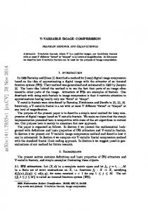
Figure 2. Multiple scan chains and slices

10%

m=3

slice 0

m=5

Figure 1. Encoding statistics for s15850

used, as l decreases, the percentage of the unencoded data bits is reduced but the total number of required codewords increases rapidly. When three different block sizes are used, the percentage of unencoded test data bits remains very low, approaching that of the smallest fixed-length-block case, with less than half of the codewords. As a result, fewer data are required for encoding the test set. III. PROPOSED ENCODING/ DECODING A. Encoding Method In the proposed approach, as test set part we consider a whole slice or a slice portion (see Figure 2, where Nsc denotes the number of scan chains, and Wsc the maximum scan-chain length). Each Huffman codeword encodes a distinct block of a specific size. When a codeword is decoded, the corresponding distinct block is generated in parallel (after codeword identification), exploiting in this way the parallelism offered by the multiple scan chains of a core. Note that for selecting the m distinct blocks that will be encoded, the x values of the test set should be first replaced by constant binary values (0s and 1s). For determining the proper x-bit assignment so as the occurrence frequencies of the encoded distinct blocks to be as skewed as possible, we use an extension of the second of the algorithms (Alg2) proposed in [23]. According to the original algorithm of [23], the two most frequently occurring test set parts that are compatible are merged, forming a more specified and frequently-occurring part than its predecessors. The same procedure is repeated iteratively until no further merging is possible. If, after the parts' merging, there are any remaining x bits, they are filled with random values. In this way, the various test set parts are gradually transformed into fully specified blocks, and the m most frequently occurring ones are selected for encoding (they constitute the set of encoded distinct blocks). The extensions on the original algorithm will become clear in the following paragraphs, during the description of the proposed approach. Initially the test set is partitioned into slices according to the scan-chain structure of the core. Each slice is also called a P0part of the test set. All P0-parts are considered for the selection of the first distinct blocks that will be encoded (P0-blocks), with size equal to the number of scan chains (Nsc). The first selected P0-block is the one that is compatible with most of the P0-parts, the second selected P0-block is the one compatible with most of the P0-parts that have not been

encoded by the first P0-block, etc. (the selected P0-blocks are derived by merging the most frequently occurring P0-parts, as explained above). When a number of P0-blocks have been selected, each one of the unencoded P0-parts is partitioned into two portions of equal size, which are called P1-parts. The size of each P1-part is equal to Nsc/2. In the case that P0-parts cannot be partitioned into two equal parts, then half of the P1parts are 1-bit shorter than the rest. Again, a number of distinct P1-blocks are selected, the unencoded P1-parts are partitioned into P2-parts and some P2-blocks are selected, the unencoded P2-parts are partitioned into P3-parts and so on. Finally, each of the P0-, P1-, ..., Pmax-blocks are compatible with some P0-, P1-, ..., Pmax-parts respectively, where the max value is determined by the designer. The Pmax-parts are also called primitive parts, since they are the smallest test set parts (and the Pmax-blocks are the smallest encoded distinct blocks). Note that each Pi-part has size equal to either ⎡Nsc/2i⎤ or ⎣Nsc/2i⎦ bits. According to the above procedure, when a test-set's Pi-part (i∈[0, max], i=0 implies a whole slice) is compatible with one of the selected Pi-blocks, then the codeword corresponding to that Pi-block is appended to the compressed test set (i.e., the Pi-part is encoded). If no encoding is possible, the Pi-part is partitioned into two Pi+1-parts, which are used for the selection of the Pi+1-blocks (and thus they may be encoded by Pi+1-block codewords). It is obvious that during the encoding of P0-parts by P0-blocks, the most sparsely specified parts are encoded, whereas the most densely specified ones are partitioned into P1-parts (since densely specified parts have small occurrence frequencies and are not selected during the parts merging procedure). In the same way, the most sparsely specified P1parts are encoded by P1-blocks, whereas the most densely specified ones are partitioned into P2-parts, etc. In other words, as also mentioned in Section II, large distinct blocks are used for encoding sparsely specified test-set regions, whereas small distinct blocks are used for the encoding of densely specified regions. As a result, the large blocks, which are derived by the merging of large test set parts, contain many x values. Instead of randomly replacing these values as in [23], we initially leave them unspecified and we utilize them later so as to increase the selected blocks' encoding ability (and hence, for further skewing their occurrence frequencies). This is done by using the codewords of the already selected blocks for encoding smaller test set parts (codeword reusability). More formally, the proposed variable-to-variable Huffman encoding procedure is further improved by allowing a Pj-part to be encoded by the codeword of a larger Pi-block (i < j), provided

4 that the first (⎡Nsc/2j⎤ or ⎣Nsc/2j⎦) bits of the Pi-block are compatible with the Pj-part (i.e., the smaller parts are always compared against the upper segments of the already selected larger blocks). Thus, the upper segments of the selected Piblocks are initially left partially unspecified and are defined later during the encoding of Pi+1-, Pi+2-, ..., Pmax-parts (in fact, contrary to [23], no random x-bit replacement is performed even in the lower segments of the selected Pi-blocks – any remaining x bits in them after the encoding process are filled with 0s and 1s by the logic synthesis tool in such a way so as the hardware overhead of the decompressor to be minimized). It is obvious that during the decoding process, only the necessary bits of the Pi-block will be generated, whereas the rest will be discarded. As an example, consider that each slice is eight bits long (Nsc = 8), and that one of the selected P0blocks is b = 00x11010. The codeword of block b can be used for encoding P1-part p = 0x11, since p is compatible with the first four bits of b. This also leads to the replacement of the x bit of b by logic value 1. With the above encoding strategy, the codeword of a P0-, P1-, ..., Pmax-1-block can be used for encoding test set parts of various sizes. Consequently, during the decoding process, every such codeword must uniquely specify the actual encoded test set part. In order to keep the compressed-data volume low, no information is stored about the size of the part encoded by a block's codeword. Instead, the encoding process is constrained according to the following condition: Condition 1: "A Pi-block codeword can be used for encoding a smaller Pj-part (j > i), if the Pj-part is not the first of a larger test set part." For example, the codeword of block b can be used for encoding a P0-part (i.e., a whole slice - all of its bits will be generated during decoding). It can be also used for encoding the second P1-part that has resulted from the partitioning of a P0-part (then the first four bits of b will be decoded). Similarly, it can be used for the encoding of the second P2-part of a P1part (the first two bits of b will be decoded). Note however that block b cannot be utilized for the encoding of the first P1part of a P0-part, or of the first P2-part of a P1-part, even if its corresponding segments are compatible with those parts. As will be seen in the following sections, by constraining the encoding process according to Condition 1, we can easily determine, during decoding, the size of the part encoded by the received codeword, by just examining the value of a small counter (a small combinational circuit along with the counter is required in terms of hardware overhead). As mentioned earlier, compression improves when every codeword encodes the largest possible test set part (since in this way, the test set will be eventually partitioned into fewer parts and therefore the total number of codewords in the compressed test set will be smaller). This means that, if possible, every test set part should be encoded before it is partitioned into smaller parts or, in other words, every selected distinct block should be used for the encoding of as many large test set parts as possible. This is why P0-parts are

1. Find the first best P0-block (the one compatible with most P0-parts) and encode all possible P0-parts (this step is for selecting at least one P0-block). 2. Set i = 0. 3. Find the next best Pi-block and calculate TestBitsi. 4. If i=max encode all possible Pi-parts using the Pi-block and go to Step 6. 5. Calculate TestBitsi+1 (considering the already chosen P0-, P1-, ..., Pi-blocks and the first Pi+1-block to be selected). If TestBitsi+1 ≥ F⋅TestBitsi, then: a) Encode all possible Pi+1-parts using the already chosen P0-, P1-, ..., Piblocks, and b) select the first (best) Pi+1-block and encode all possible Pi+1-parts that have remained unencoded after substep 5a. Also, set i=i+1. Else: Select the Pi-block and encode all possible Pi-parts using the Pi-block. 6. If the number of selected distinct blocks does not exceed a predetermined upper limit, go to Step 3. 7. Label all unencoded Pmax-parts as failed. 8. Generate the Huffman code and produce the compressed test set. Figure 3. Proposed encoding algorithm

encoded first, then P1-parts, P2-parts, etc. Furthermore, we do not allow the encoding of a Pi+1-part (i ∈ [0, max-1]) by the codeword of a larger P0-, P1-, ..., Pi-block, before the beginning of the encoding process of Pi+1-parts. For example, the encoding of a P3-part by a P0-block codeword, before the selection of P1- and P2-blocks, is not allowed. The reason is that this encoding may prevent a possible subsequent encoding of a (larger) P1- or P2-part that includes the aforementioned P3-part. The encoding process of Pi-parts stops and that of Pi+1-parts begins when the total number of bits of the Pi-parts (TestBitsi) that are compatible with the next Pi-block to be selected, are fewer by a factor F than the bits of the Pi+1-parts (TestBitsi+1) that can be encoded by: a) the codewords of the already chosen P0-, P1-, ..., Pi-blocks, and b) the codeword of the first Pi+1-block to be selected (i.e., when TestBitsi+1 ≥ F ⋅ TestBitsi). Factor F is used for achieving a balanced selection between large and small blocks. When switching from Pi-parts to Pi+1parts, the block size is halved (and hence, as explained in Section II, more test data can be encoded), but the number of codewords for encoding the same test-data volumes is doubled. In other words, TestBitsi+1 are expected to be more than TestBitsi most of the times, but this does not guarantee better compression, since the double number of codewords is required for encoding the same number of bits. Thus, assuming that all codewords have the same length, TestBitsi+1 must be at least twice as many as TestBitsi (F = 2) for switching from Piparts to Pi+1-parts. However, F values greater than 2 may be preferable, since the codewords of the larger blocks are generally smaller than those of the smaller blocks, due to their higher occurrence frequency (which is a result of their increased reusability). The F value that maximizes the compression ratio for each circuit (a small positive integer greater than 1) can be easily tracked down since the running time of the encoding method is very short, and the set of possible F values is very small. Note that without factor F, the proposed encoding algorithm would have selected very few large blocks and many small blocks. When all P0-, P1-, ..., Pmax-blocks have been selected (their total number m is defined by the designer according to the area overhead constraints of the design), some of the Pmax-

Nsc=8

5

X 0 1 X X 0 1 X

X 1 1 X X X 1 X

X X 0 X X 1 0 0

0 1 0 X X X X X

X X 0 1 1 0 0 X

1 X 1 X 0 X 1 0

0 X 1 X X X X 0

1 1 1 1 0 1 1 1

P0

P0

P0

P0

P0

P0

P0 P0

P0

2P1 P0 2P1 2P1 2P1 2P1 2P1

X 1 1 X X X 1 X

X X 0 X X 1 0 0

0 1 0 X X X X X

X X 0 1 1 0 0 X

1 X 1 X 0 X 1 0

0

P1-block = 1111

4/20

110

P2-block = 01

6/20

10

failed

1/20

111

X 0 1 X X 0 X X

1 11/ 20

0

1 0

5/20

0 P0

9/ 20

P2 6/20

(d)

P1 4/20 (e)

1 fail. 1/20

X 1 1 X X X 1 X

X X 0 X X 1 0 0

P0 2P1 4P2

(c)

0 1 0 X X X X X

X X 0 1 1 0 0 X

1 X 1 X 0 X 1 X

failed

Encoded data volume = 38 bits Compr. Ratio = 40.6 % Encoded Test Data 4P2 2P1

1

9/20

P0

1 1 1 1 0 1 1 1

20/ 20

occur. Code freq. word

P0-block = 00100010

0 X 1 X X X X 0

2

(b)

(a) Encoded distinct blocks

X 0 1 X X 0 X X

+P 2 2P

1 1 1 1 0 1 1 1

P +2 P1

0 X 1 X 0 X X 0

0 1 0 1 1 1 1 1 1 0 0 0 0 0 0 0 1 1 0 1 0 0 0 0 1 1 0 1 1 1 0 1 0 0

1 1 0 0

(f)

Figure 4. Proposed encoding example

parts remain unencoded. Such parts are labeled as failed and a separate Huffman codeword is assigned to all of them. In the compressed test set, these Pmax-parts are embedded unencoded, preceded by the aforementioned codeword. The Huffman tree is constructed when all Pi-blocks for (i=0, 1, ..., max) have been selected, so as all occurrence frequencies to be known. An overview of the proposed algorithm is shown in Figure 3. We illustrate the above described process with the following example: Example 1. Consider a circuit with Nsc=8 scan chains. Each slice can be partitioned into at most four P2-parts of 2 bits (max=2, P2-parts are primitive parts). The 64-bit test set shown in Figure 4a is initially partitioned into P0-parts. Since all P0parts appear only once in the test set (an x value is considered different from a 0 or an 1), the first two that are compatible (0x1x0xx0 and x01xx01x) are merged. The resulting part (001x0010) is compared against all the rest P0-parts and since it cannot be merged with any of them, it constitutes the first P0-block. The P0-parts encoded by this P0-block are highlighted in Figure 4a. Assume now that factor F has been set to such a value that the encoding of P0-parts (selection of P0-blocks) has to stop and the encoding of P1-parts (selection of P1-blocks) has to begin. Therefore, the unencoded P0-parts are partitioned into P1-parts. This is illustrated in Figure 4b (note that in each figure representing a step of the encoding algorithm, every already encoded part is shown in light grey). Before selecting the first P1-block, all P1-parts which are compatible with the first half of the selected P0-block and, at the same time, satisfy Condition 1 (i.e., the second P1-parts of all P0-parts) are encoded by using this block (these P1-parts are boldfaced and underlined in Figure 4b). Note that by using the first half of P0-block 001x0010 for encoding the P1-part 0x10, the unspecified bit of the P0-block is set to 0. Then, the first P1-block has to be selected. Since all the remaining P1-parts appear only once, the first two that are compatible (i.e., 1111 and x11x) are merged. The resulting part (1111) can be also

merged with P1-part 1x1x. Thus, 1111 constitutes the first selected P1-block and the P1-parts that are encoded using this block are highlighted in Figure 4b. Assume again that after this step, inequality TestBitsi+1 ≥ F⋅TestBitsi is true and as a result the encoding of P1-parts stops and that of P2-parts begins. After partitioning all unencoded P1-parts into P2-parts (Figure 4c), all P2-parts which satisfy Condition 1 and are compatible with the first quarter of the selected P0-block (00) as well as with the first half of the selected P1-block (11) are encoded by using the corresponding blocks (they are boldfaced and underlined in Figure 4c). Then, P2-part 01, which appears three times, is merged first with P2-part xx that appears twice, and next with P2-part x1. The resulting part (01) is the first selected P2-block and the P2-parts encoded by this block are highlighted in Figure 4c. One P2-part (10) is left unencoded as shown in Figure 4c and is labeled as failed. Note that when the encoding process is complete, the test set has been partitioned into totally 20 P0-, P1- and P2-parts. In Figure 4d the selected distinct blocks, their occurrence frequencies and the corresponding Huffman codewords generated by constructing the Huffman tree of Figure 4e are reported. Finally in Figure 4f the encoded test set is shown with the last bit of each codeword underlined and the unencoded test set part (10) ■ boldfaced and italicized. We note that for small part sizes (up to 12 bits), instead of using the heuristic proposed in [23] for merging the various test set parts, optimal part merging (in terms of occurrencefrequency skewing of the selected distinct blocks) can be achieved as follows: assuming part size of k bits, all test set parts are examined against all 2k fully specified patterns of k bits (00...00, 00...01, ..., 11...11). The pattern that is compatible with most test set parts is found and these test set parts are merged for constructing the first selected block. Then we find the pattern that is compatible with most of the remaining parts, which are merged for forming the second selected block, and so on.

6 Pi-block corresponding to the received codeword

P0

P1

P2

P3 = = Pmax

Primitive # of 0 s Parts LS bits (max–i = 3) (max–i = 2) (max–i = 1) (max–i = 0) 0 000 3 23 / 0-7 22 / 0-3 21 / 0-1 20 / 0

Slice

8 bits

1

001

0

20 / 1

20 / 1

20 / 1

20 / 1

2

010

1

21 / 2-3

21 / 2-3

21 / 2-3

20 / 2

3 4 5 6 7

max=3

011 100

0

20

2

2

/3

2 / 4-7

/3

2

2 / 4-7 0

20

/3

1

2 / 4-5 0

20 / 3 20 / 4

0

2/5

2 /5

2 /5

20 / 5

110

1

1

2 / 6-7

1

2 / 6-7

1

2 / 6-7

20 / 6

111

0

20 / 7

20 / 7

20 / 7

20 / 7

101

0

20

# of decoded Pmax-parts / positions of decoded Pmax-parts

Figure 5. Decoding method example

B. Decoding Method In this section we describe the way that test set parts are generated from the received codewords during the decoding process. Every slice consists of 2max primitive parts (Pmaxparts), and thus the size of a P0-part (slice) or P0-block is equal to that of 2max primitive parts, the size of a P1-block is equal to that of 2max-1 primitive parts, etc. The decoding of every slice begins from the first primitive part (i.e., primitive part 0) and continues with primitive parts 1, 2, …, 2max-1. Note however that depending on the received codeword and the status of the decoding process, a test set part larger than a primitive one (with size equal to that of multiple primitive parts) can be generated every time. When a whole slice has been produced, it is loaded into the scan chains and the decoding of the next slice begins. Let s be the value of a counter, consisting of max bits, which points to the next primitive part of a slice that has not yet been decoded. The first task of the decoding process is to determine the size L of the largest possible test set part that can be decoded, irrespectively of the received codeword. This can be easily done by examining the value of s. Specifically, the largest possible test set part that can be decoded is a P0part only if s is divided exactly by 2max, or equivalently if the max least significant bits of s are all equal to 0. If s is not divided exactly by 2max, the largest possible test set part that can be decoded is a P1-part only if s is divided exactly by 2max-1, or equivalently if the max-1 least significant bits of s are all equal to 0. Therefore, the largest possible test set part that can be decoded is a Pi-part if s is divided exactly by 2max-i but not by 2max-i+1, or equivalently if the volume of consecutive least significant bits of s that are 0 is equal to max-i. The second task is to examine the received codeword and determine the size of the distinct block it encodes. If the size of the distinct block corresponding to the received codeword is smaller or equal to the size L of the largest possible test set part that can be decoded (according to the value of s), then the actual test set part that will be decoded is identical to the whole distinct block. If the size of the distinct block is larger than L, then the upper L bits of the distinct block are decoded. Suppose for example that the largest possible test set part that can be decoded (according to the value of s) is a Pi-part. Then upon reception of a codeword corresponding to a Pi-, Pi+1-, ..., Pmax-block, the decoded test set part is identical to the whole Pi-, Pi+1-, ..., Pmax-block, respectively. On the other hand, upon

reception of a codeword corresponding to a P0-, P1-, ..., Pi-1block, the upper segment of the P0-, P1-, ..., Pi-1-block, respectively, with size equal to that of the Pi-part, will be decoded. In order to better clarify this process we present the following example. Example 2. Consider a circuit with Nsc=64 scan chains. Each slice of the test set is 64 bits long and includes 23=8 primitive parts. Hence max = 3 and each primitive part consists of 8 bits. The test set of the circuit is encoded using P0-, P1-, P2-, and P3-blocks, of size equal to that of 8, 4, 2 and 1 primitive part, respectively. In Figure 5 we present a slice partitioned into 8 Pmax-parts (0-7), as well as the values of s, which indicate the next primitive part of the slice that will be decoded (note that when s=000, no Pmax-part has been decoded yet). Suppose that during the decoding process, a codeword encoding a P1-block is received (i=1). If s=0 (000) or s=4 (100), then s is divided exactly by 2max-i=22, and therefore the whole P1-block is loaded in the positions of the next 22 primitive parts (0-3 when s=000, or 4-7 when s=100). If s=2 (010) or 6 (110), then s is not divided exactly by 2max-i, but by 2max-i-1 = 21, and therefore the first half of the P1-block is loaded in the positions of the next 21 primitive parts (2-3 when s=010, or 6-7 when s=110). Finally, if s=001, 011, 101 or 111, s is divided exactly only by 2max-i-2=20, and thus the first quarter of the P1-block is loaded in the position of the next 20 primitive part (1, 3, 5 or 7, when s=001, 011, 101 or 111, respectively). As we have mentioned earlier, the portion of the P1-block that will be decoded can be straightforwardly determined by examining the volume of consecutive least significant bits of s that are 0 (if 2 LS bits are 0 then 22 Pmax-parts will be decoded, if 1 LS bit is 0 then 21 Pmax-parts will be decoded, etc.). In Figure 5, for every possible combination of s, i, we show the number and the positions of the Pmax-parts that will be decoded. This table can be easily constructed in the same systematic way for every value of Nsc and max. ■ C. Statistical Improvement of Test Data In this section, we propose two simple test-set transformations, which can be optionally applied before compressing the test data, for improving their statistical properties (no structural information of the core is required). Both transformations increase the difference between the volumes of 0s and 1s in the test set in order to skew the probability of occurrence of one of them (either 0 or 1). In this way the probability of occurrence of every Pi-block is skewed, and therefore the compression ratio increases even more. The following two transformations are proposed: T1: Inversion of all test data bits of selected scan chains. T2: Inversion of the test data bits of selected scan cells. Both transformations are applied to the test set before it is encoded. The transformed test set is then compressed and during decompression the original test set is restored by removing on the fly the transformations. At first, for each scan cell c ∈[0, Wsc-1] of every scan chain s ∈[0, Nsc-1], we calculate the volume of 0s and 1s ( Vs0,c and

7 Wsc

ATE Data

Send

Huffman FSM Failed

Distinct Block

Nsc

Nsc Rin

Register

Input Buffer

ATE Channels

CodeIndex

Data In

Invert Unit

ATE_CLK

Nsc

Nsc

Rout

Valid Code Ready Size Part 2max Size/ Enable EN

ATE_Sync

Core

slice 0

Slice Counter

slice Wsc-1

Figure 6. Proposed decompression architecture

Register

Vs1,c respectively) that appear at the corresponding position of all the test-set's cubes (an s, c pair defines a unique position in the test cubes). The 0- and 1-bit volumes for each scan chain are equal to V = 0 s

Wsc −1

∑V c=0

0 s,c

and V = 1 s

Wsc −1

∑V c=0

1 s,c

, while the total

number of 0s and 1s in the test set is calculated as

V0 =

N sc −1

∑V s =0

0 s

and V 1 =

N sc −1

∑V s =0

1 s

. Assume, without loss of

generality, that for a test set, the 0-bit volume is higher than the 1-bit volume (V0 > V1). According to T1, the scan chains with more 1s than 0s (considering all test vectors) can be inverted, for favoring the 0s count. This transformation is very simple and for reversing it, only one inverter is required for each scan chain with inverted values. Similarly, T2 can be used for inverting the values of a predefined number of scan cells with the highest difference of 0-bits from 1-bits ( Vs1,c - Vs0,c ) for all test vectors. Both transformations improve, in most cases, the compression ratio, while they impose very small hardware overhead. IV. PROPOSED ARCHITECTURE The proposed decompression architecture is presented in Figure 6. It consists of the following units: Input Buffer: This unit synchronizes the communication between the ATE and the decompressor. It receives the encoded data from the ATE channels in parallel with the frequency of the ATE clock (ATE_CLK), and shifts them serially into the Huffman FSM with the frequency of the system clock. When encoded data have been received from the ATE, Input Buffer notifies the Huffman FSM (Ready = 1), which controls their shift with signal Send. When Input Buffer empties, signal Ready is reset (Ready = 0) until new data are received from the ATE. The flow control between the Buffer and the ATE is performed via signal ATE_Sync. Huffman FSM: It is a finite state machine which receives serially the data from the Input Buffer. When the Huffman FSM recognizes a codeword, and assuming that the implemented code consists of N codewords, it places on the bus CodeIndex a binary index (value) between 0 and N-1. This index indicates which codeword has been received (Valid

Rin(0...7) EN0 Rin(8...14) EN1 Rin(15...22) EN2 Rin(23...29)

8 7 8 7

EN3 Rin(30...37)

8

EN4 Rin(38...44)

7

EN5 Rin(45...52)

8

EN6 Rin(53...59)

7

G0 G1 G2 G3 G4 G5 G6 G7

8 7 8 7 8 7 8 7

Rout(0...7) Rout(8...14) Rout(15...22) Rout(23...29) 60 Rout(30...37) Rout(38...44) Rout(45...52) Rout(53...59)

EN7

Figure 7. Register unit example

Code is also set to 1). When the received codeword corresponds to an unencoded (failed) data block, the Huffman FSM sets signal Failed=1 as well. Register: The Register unit consists of a number of flip-flops, equal to the number of scan chains Nsc, which are partitioned into groups. Each flip-flop group corresponds to a primitive (Pmax-) part and is controlled by an enable signal (one of the signals of bus EN) activated by the Part Size/Enable unit. According to the proposed encoding scheme, the number of Pmax-parts per slice is 2max. Every P0-, P1-, P2-, ..., Pmax-part has length equal to that of 2max, 2max-1, 2max-2, ..., 20 Pmax-parts respectively. Therefore, during the decoding of a Pi-part, 2max-i successive groups of the Register are concurrently loaded. Example 3. Let Nsc=60 and thus the size of the various test set parts is: P0-parts = 60 bits, P1-parts = 30 bits, P2-parts = 15 bits and P3-parts = Pmax-parts = 8 and 7 bits. The corresponding Register is shown in Figure 7. It comprises 4 groups of 8 flip-flops (G0, G2, G4 and G6) and 4 groups of 7 flip-flops (G1, G3, G5 and G7). During the generation of a P0part (60 bits), all enable signals EN0...EN7 are concurrently activated and the Distinct Block unit provides the 60 bits of the decoded P0-block at the inputs Rin(0...59). When a P1-part (30 bits) has to be loaded, then, according to the partitioning of each slice, either signals EN0...EN3 or EN4...EN7 are activated, while the required 30-bit block is duplicated by the Distinct Block unit (as we will see shortly) so as to be present

8 at the Rin(0...29) as well as at the Rin(30...59) Register inputs. Similarly, during the generation of a P2-part, the proper from the four copies of a 15-bit block is selected by activating signals EN0, EN1 or EN2, EN3 or EN4, EN5 or EN6, EN7 [the same 15-bit block is available at the inputs Rin(0...14), Rin(15...29), Rin(30...44) and Rin(45...59)]. Finally, for a P3-part (8 or 7 bits), one of the signals EN0, ..., EN7 is activated and the Distinct Block unit provides the same 8-bit data block at the inputs Rin(0...7), Rin(8...14), Rin(15...22), Rin(23...29), Rin(30...37), Rin(38...44), Rin(45...52) and Rin(53...59) (note that in the case of a group with 7 bits, the 8th bit of the block is ■ simply ignored). We have to mention here that Register unit can be omitted if the core provides a separate scan-enable signal for each scan chain. Then signals ENj are connected to the proper scanenable signals, and the signals which drive the inputs of the register will be directly connected to the scan chains. Part Size/Enable Unit: It is a small combinational circuit which determines the size of the test set part that is encoded by the received codeword (in primitive-parts multiples), and enables the groups of the Register that will be loaded by activating the respective ENj signals. According to the proposed approach, even if a codeword corresponds to a Piblock, it may be utilized for encoding Pi+1, Pi+2, ..., Pmax-parts (with sizes equal to that of 2max-i-1, 2max-i-2, ..., 20 primitive parts). The portion of the block that will be decoded is determined by the value (s) of a binary counter embedded in this unit, as well as by the received codeword (see Example 2). s ranges from 0 to 2max-1, pointing to the next primitive part of a slice that has not been decoded yet. Specifically, assuming that a codeword corresponds to a Pi-block, if s is divided exactly by 2max-i then the whole Pi-block is decoded. Consequently, the next 2max-i groups are loaded in parallel (enable signals EN s , EN s +1 ,..., EN s + 2max −i −1 are activated), and the value of the counter is increased by 2max-i. If s is not divided exactly by 2max-i but by 2max-i-1, then the upper half of the Pi-block is decoded (with size equal to that of a Pi+1-part). Therefore, the next 2max-i-1 groups are loaded in parallel (signals EN s , EN s +1 ,..., EN s + 2max −i −1 −1 are activated), the value of the counter is increased by 2max-i-1, and so on. The maximum power of 2 that divides s exactly is provided by a simple combinational circuit, which determines the number of consecutive least significant bits of the counter that are 0 (s is divided exactly by 2q when the q least significant bits of s are all equal to 0). Concurrently with the activation of signals ENj, the Distinct Block unit, which receives the size of the part that will be decoded (bus Size), generates the appropriate block portion at the inputs of the Register groups. After the last group of the Register has been loaded, the counter is reset to 0. Distinct Block Unit: It is a combinational circuit which receives the CodeIndex value indicating the current codeword, as well as the size of the part that will be decoded (bus Size) and returns the proper portion of the distinct block encoded by this codeword. Specifically, if the part that will be decoded has size equal to that of 2q primitive parts (this size is provided by

the Part Size/Enable unit), then at the outputs of the Distinct Block unit, 2max-q copies of the first 2q · |Pmax| bits of the encoded distinct block are generated (|Pmax| indicates the size of the primitive parts in bits). In this way, the same data are repeated for every 2q-tuplet of Register groups, while the activated enable signals (ENj) ensure that only the proper 2qtuplet will be loaded (see Example 3). Similarly, in the case of a failed Pmax-part, data received directly from the ATE (through the Input Buffer unit) are repeated for every group of the Register. Invert Unit: This unit is optional and is inserted only when transformations T1 and/or T2 are applied to the test set. It consists of at most Nsc gates, one for each scan chain, and of a decoding logic, only when T2 is applied. When transformation T1 is employed, the required gate is an inverter that inverts all test data entering a scan chain. If transformation T2 is applied to one or more scan cells of a scan chain, an exclusive-OR or an exclusive-NOR gate is needed for selectively inverting the corresponding test bits. If we consider both transformations there are totally four cases: 1. Neither a scan chain, nor any of its cells are inverted (T1 and T2 are not applied for this scan chain). Then no logic is required for this scan chain. 2. A scan chain is inverted (T1 is applied to this scan chain), but none of its cells is re-inverted (T2 is not applied to any cell of this scan chain). Then an inverter is used for inverting all data entering the scan chain. 3. A scan chain is not inverted (T1 is not applied to this scan chain), but at least one of its cells is inverted (T2 is applied for this scan chain). Then an exclusive-OR gate is used for inverting only the bits of the selected scan cells. 4. A scan chain is inverted (T1 is applied to this scan chain), and at least one of its cells is inverted again (T2 is also applied). Then an exclusive-NOR gate is used for inverting all data entering the scan chain except for those corresponding to the cells that are inverted twice. In cases 3 and 4, the second input of the exclusive OR/ NOR gates is driven by the decoding logic, which selects the scan cells to be inverted, according to the value of the Slice Counter (it is in the range [0, Wsc-1] ). V. TEST APPLICATION TIME CALCULATION Let us now calculate the test application time of the proposed method. Suppose that ⎜E⎜ is the size in bits of the compressed test set, fATE and fSYS are the ATE and system clock frequencies respectively (with fSYS = r · fATE), Nch is the number of ATE channels that are used for transferring the compressed data, and NC, UD are the number of codewords in the compressed test set and the number of data bits that remain unencoded, respectively. The test application time (TAT) of the proposed approach consists of: a) the time for downloading the data stream from the ATE to the core, which is E , b) the time required for shifting and decoding t1 = N ch ⋅ f ATE the test data (one bit per system cycle) from the Input

9

90 89

No Transf. T1+50T2

88

T1+100T2

87 86 m = 16

m=8

m = 24

Compression Ratio (%)

Compression Ratio (%)

s13207

s9234

68 66 64 62 60 58 56 54 52 50 m=8

Selected distinct blocks

m = 16 m = 24 Selected distinct blocks

Figure 8. Effect of the selected distinct block’s volume and of Transformations T1 and T2 on the Compression Ratio

Buffer to the outputs of the Huffman FSM unit, that is E − UD , and c) the time required for loading the t2 = f SYS Register unit with the decoded blocks (one system clock per NC codeword), which is t3 = . Therefore, the total time is: f SYS

E

1 ( E − UD + NC ) (1) N ch ⋅ f ATE r ⋅ f ATE Note that since the loading of the Register unit requires only a single cycle for each distinct block, it can be overlapped with the decoding of the next codeword and thus t3 can be eliminated. However here, we do not consider this improvement in order to study the worst-case scenario. TAT = t1 + t2 + t3 =

+

VI. EVALUATION AND COMPARISONS The proposed compression method was implemented in C programming language, and experiments were performed using the dynamically compacted Mintest test sets [15] for stuck-at faults. The same test sets were also used in [7], [8], [10], [11], [13], [23], [27]-[29], [31], [39], [41], [43], [45], [47], [48], [50], [51], [55] and [56]. The run time of our method is a few seconds for each experiment. The compression ratio is calculated by using the formula: Mintest bits - Compressed bits Compression Ratio ( % ) = ⋅100 Mintest bits At first we examine how the various parameters affect the efficiency of the proposed approach. Due to the high volume of the conducted experiments, we present results only for circuits s9234 and s13207 but the results for the rest benchmarks are similar. In the first set of experiments we examine the effect of the volume of the selected variablelength distinct blocks (m), as well as of statistical transformations T1 and T2 on the compression ratio. Figure 8 presents the compression ratios of the proposed method assuming 64 scan chains for s9234 and s13207, 8, 16 and 24 variable-length distinct blocks (blocks of sizes 64, 32, 16 and 8 bits were selected in all experiments), and various values of factor F (the best ones in terms of compression ratio were used). Three different compression cases are presented for each distinct-block volume: a) compression without any transformations ("No Transf."), b) compression with

transformations T1 and T2 for 50 selected cells ("T1 + 50 T2"), and c) compression with transformations T1 and T2 for 100 selected cells ("T1 + 100 T2"). It can be seen that compression improves as the volume of distinct blocks (m) increases from 8 to 16, whereas the improvement is smaller as m increases further from 16 to 24. In fact, distinct-block volumes greater than 24 yield a very small performance boost, and for that reason, in our experiments, we utilized m values up to 24. On the other hand, the application of transformations T1 and T2 has a noticeable impact on the compression ratio, irrespectively of the volume of the selected distinct blocks. However, when the volume of the cells inverted by transformation T2 increases from 50 to 100, the compression does not improve significantly (in some cases, it even decreases slightly). This is due to the fact that there is a saturation point, after which any further increase in the number of cells inverted by T2 does not practically affect the compression ratio. Our experiments showed that compressionratio saturation is generally reached with a small number of inverted cells (50 - 100). In other words, a small number of inverted cells is sufficient for improving the statistical properties of the test set. Note that, as we will see later, the volumes of both the selected distinct blocks and the cells inverted by transformation T2 affect the hardware overhead of the decompressor as well. We therefore conclude that the selection of a small number of distinct variable-length blocks, in conjunction with the application of both transformations T1 and T2 (for a small number of selected cells, i.e., 50 - 100), provides very good compression results with small area overhead (the overhead imposed by T1 is negligible). In the second set of experiments we study the effect of factor F on the compression ratio. We remind that F is used for balancing the distribution of the sizes of the selected variable-length distinct blocks. We ran the proposed method for F = 1, 2, ..., 7 and 8, assuming 64 scan chains and 8 selected distinct blocks of lengths 64, 32, 16 and 8 bits. The compression ratios of these experiments for the test sets of s9234 and s13207 are presented in Figure 9. As expected, the compression ratio initially improves as F becomes greater than 1, it reaches a peak value and then it drops. The peak value corresponds to the distinct-block-sizes distribution with the highest efficiency. Taking into account that the run-time of the proposed method is very short, the designer can quickly track

10 TABLE II. COMPARISONS AGAINST COMPRESSION METHODS FOR CORES WITH MULTIPLE SCAN CHAINS Select. Proposed (# bits) Reduction %* of proposed over: Mintest [29] [41] [47] Circuit Huff. No T1 + Min- Select. (# bits) (# bits) (# bits) (# bits) [29] [41] [47] (# bits) Transf. 100 T2 test Huff. 23754 11433 9247 14220 8736 68.0 33.4 17.7 46.5 s5378 7611 39273 19168 15722 30144 14493 67.5 33.4 18.8 57.7 s9234 12765 91.2 48.5 19.7 30.5 80.4 s13207 165200 28328 18153 20988 74423 16193 14578 78.5 38.4 14.2 34.1 36.4 s15850 76986 26873 19313 25140 26021 18611 16562 59748 64.4 17.3 0.1 31.2 -30.4 s38417 164736 70954 58706 85225 45003 58663 72.2 22.4 4.2 3.1 24.7 s38584 199104 71315 57801 57120 73464 55612 55353 *Reduction % = [1 - (# bits of best proposed / # bits of: Mintest, Select. Huff., [29], [41], [47]) ] · 100

s5378 s9234 s13207 s15850 s38417 s38584

90 80

s9234 s13207

70 60 50

16

32 64 Number of Scan Chains (Nsc)

128

Figure 10. Effect of Nsc on the proposed encoding

100 s13207

s9234

90 Compression Ratio (%)

100 Compression Ratio (%)

Circuit

TABLE I. RESULTS OF THE PROPOSED ENCODING (# BITS) 16 Scan Chains 64 Scan Chains 128 Scan Chains No No T1 + T1 + No T1 + T1 + T1 + T1 + Transf. 50 T2 100 T2 Transf. 50 T2 100 T2 Transf. 50 T2 100 T2 9776 9183 8955 8736 8267 8384 9277 7611 7611 15792 14514 14049 14565 13265 13164 14493 12765 12765 24039 23053 21623 17911 16748 16366 16193 15092 14578 22113 20685 20016 19570 18161 17595 18611 17354 16562 58663 61241 59748 59411 64262 63165 59492 64963 63833 60291 60101 59809 56890 57309 56854 55612 55965 55353

F=1 80

F=2 F=3

70

F=4 F=5

60

F=6 50

F=7 F=8

40 30 No Transf.

T1+50T2

T1+100T2 No Transf.

T1+50T2

T1+100T2

Figure 9. Effect of factor F on the proposed encoding

down the best value of F for each case (a small positive integer greater than 1). Another factor that affects the efficiency of the proposed approach is the slice size, i.e., the number of scan chains (Nsc) of the CUT. Figure 10 presents results for Nsc=16, 32, 64 and 128, assuming 24 selected distinct blocks of variable lengths. The size of the primitive parts was set to 8. No test-set transformations were applied, in order to focus solely on the compression method. Various values of factor F were examined and the best one was selected for each core. We can see that as the number of scan chains (and thus the slice size) increases, the compression ratio improves. This is an expected behavior, if we consider how the test set is partitioned into parts; when the number of scan chains is doubled, the number of available part/block-sizes increases (note that the size of the primitive parts remains the same). As a result, the encoding ability of the proposed method improves (due to the greater block-size granularity). In Table I we present the test-data compression results (# bits) of the proposed method for 16, 64 and 128 scan chains and 24 selected distinct variable-length blocks (the bit volumes of the original Mintest test sets can be found in Table II). The size of the primitive (Pmax-) parts was equal to 8 bits in all

experiments (since Pmax-parts are the smallest encoded test set parts, their size should be similar to the block size of simple Selective Huffman coding [23], [28]). In almost all cases compression improves as the number of scan chains increases. Also, compared to the "No Transformations" case, almost always we get better compression when T1 + 50 T2 are applied, whereas, most of the times, a further increase in the number of cells inverted by T2 does not provide significant improvements. Also, as explained earlier, there are a few cases, where no increase or even a marginal drop on the compression ratio is observed when the number of inverted cells increases from 50 to 100 (e.g., s5378 for 64 scan chains). We next compare the proposed approach against methods that also exploit the multiple scan chains of a core for reducing the test application time. Note that no comparisons are provided against approaches that need structural information of the CUT or require ATPG and/or fault simulation synergy. Such methods target cores of known structure and thus employ fault simulation, and, most of the times, specially constrained ATPG processes, which reduce significantly and tailor to the encoding method the data that need to be compressed. We mention that for cores of unknown structure neither ATPG nor fault simulation can be performed. Also, we do not compare against: a) the approach of [12], since several conditions have to be satisfied by a core nearby the CUT, so as the former to be used as decompressor, and b) methods that provide results for different test sets from those used in our experiments. The compressed data volumes are significantly affected by the utilized test sets and therefore no conclusions can be drawn by such comparisons. In Table II, comparisons against Mintest, selective Huffman [23] (re-implemented here for multiple – i.e., 64 – scan chains), [29], [41] and [47] are presented. In column 2, we provide the sizes

11 TABLE III. COMPRESSION RATIOS (%) OF THE PROPOSED AND DICTIONARY-BASED

800

METHODS

[31] 70.3 81.7 76.3 70.6 75.1

[39] 73.3 70.7 94.8 82.0 61.8 73.2

[50] 90.0 88.8 95.4 92.6 70.5 87.9

[51] 63.2 61.0 89.2 75.9 71.4 73.8

[55] 61.0 55.0 81.5 79.0 61.6 60.0

[56] 51.2 51.9 80.8 64.0 48.5 67.2

Prop. 68.0 67.5 91.2 78.5 64.4 72.2

TABLE IV. PROPOSED VS. METHODS FOR SINGLE-SCAN-CHAIN CORES (REDUCTION %) Circuit [7] [8] [10] [11] [13] [23] [27] [28] [43] [45] [48] [51] - 34.9 38.4 33.5 28.6 18.7 20.7 33.3 30.7 47.9 27.6 s5378 s9234 42.6 43.3 40.9 42.4 38.4 29.0 17.7 18.6 39.9 38.0 46.7 28.1 s13207 65.0 58.5 55.3 52.8 46.5 61.6 20.7 39.9 51.4 49.5 61.6 40.4 s15850 59.3 45.8 37.0 36.3 32.9 36.7 12.5 22.7 32.8 34.1 47.1 25.1 s38417 36.3 35.6 9.7 37.2 23.6 13.1 0.2 -0.2 9.7 0.6 20.1 4.0 s38584 46.8 38.4 28.5 28.9 26.3 22.6 -0.3 8.9 25.0 26.1 35.9 12.0

of the original Mintest test sets. For the selective Huffman approach, the number of selected fixed-length distinct blocks was set to 24 and three different block sizes equal to 8, 16 and 32 bits were examined. The best result for every circuit is reported in column 3 of Table II. Columns 4, 5 and 6 present the best results of [29], [41] and [47] respectively. Note that for the approach of [47], apart from the test data reported in column 5, an additional significant amount of control data should be stored in the ATE and then transferred to the CUT. Although these additional data increase the volume of the stored bits, they cannot be taken into account in Table II, since they have not been reported by the authors of [47]. In columns 7 and 8 we provide the best results of the proposed method when transformations T1 and T2: a) are not applied (column 7), and b) are both applied (T2 for 100 selected cells – column 8). Finally, columns 9-13 report the reduction percentages of the proposed method (considering the best-boldfaced results of columns 7 and 8) over the rest methods. As we can see, in all but one case (s38417 of [47], for which no control data have been reported) the proposed technique performs better than the others. In Table III we provide the compression ratios achieved by dictionary-based methods suitable for cores with multiple scan chains (columns 2-7), as well as those achieved by the proposed approach (column 8). In some cases our method performs better than the rest, whereas in others it does not. However, as we will show later, the hardware overhead of dictionary-based methods is prohibitively large. In Table IV we present the compressed-data reduction percentages of the proposed method against techniques applicable to cores with a single scan chain. The compression achieved by the proposed approach is higher than that of the rest methods, except for the s38584 case of [27] and the s38417 case of [28] which are marginally higher. Note that all these methods require long test application times due to their inability to exploit the parallelism of multiple scan chains. For assessing the hardware overhead of the proposed method, we synthesized three different decompressors for the test set of s9234, applying: a) no transformations, b) T1 and T2

700 Gate Equivalents

Circuit s5378 s9234 s13207 s15850 s38417 s38584

Selective Huffman

Proposed

600

Select. Huff. BS=8

500

Select. Huff. BS=16 Select. Huff. BS=32

400

Prop. No Transf.

300

Prop. T1 + 50 T2

200

Prop. T1 + 100 T2

100 0

BS=8

BS=16

BS=32

No Transf. T1+50T2

T1+100T2

Figure 11. Hardware overhead for 24 selected distinct blocks

for 50 selected cells, and c) T1 and T2 for 100 selected cells. We also synthesized the decompressor of the implemented parallel selective Huffman approach, with (fixed) block size (BS) equal to 8, 16 and 32. In all experiments, the number of scan chains was set to 64, and the number of selected distinct blocks to 24 (note that the decompressor size does not depend on the compressed test set, but on architectural parameters like the number of scan chains, the number of selected distinct blocks, the number of selected cells in transformation T2, etc.). The results are shown in Figure 11 in gate equivalents (a gate equivalent corresponds to a 2-input NAND gate). Observe that the transformations marginally increase the hardware overhead of the proposed method. Compared to the well-known selective Huffman approach, the proposed one imposes slightly higher hardware overhead. The hardware overhead of [29] for 24 selected cells is 582 gate equivalents and thus it is very close to the hardware overhead of the proposed method. As far as the approaches of [41] and [47] are concerned, their hardware overhead is low, but, as shown earlier, their compression ratios are much smaller than those of the proposed method. Compared to the dictionary-based methods, the hardware overhead of the proposed approach is very small. The size of the required dictionary in [51] is in the range of 1,187 to 9,152 bits, which is comparable to that of [39] and smaller than those of [31] and [55]. The size of the dictionary in [56] is between 6,264 and 43,712 bits, while that of [50] is equal to 25,600 bits. Apart from the dictionaries, extra area will be also occupied by the decompressors of the above techniques. Therefore, we conclude that dictionary-based methods impose prohibitively large hardware overhead. The hardware overhead of the single-scan-chain methods, in gate equivalents, is: 125-307 for [7] (as reported in [13]), 320 for [10], 136-296 for [13], 203-432 for [27], 551-769 for the main part of the decompressor in [45] and 416 for [51]. The hardware overhead of [23] is greater than that of [13]. Although cheaper in hardware, these techniques require much longer test application times and much more data to be stored in the ATE, compared to the proposed approach. As far as the test application time (TAT) is concerned, the reduction percentages of the proposed method, assuming 5 ATE channels, are shown in Figure 12 (we considered the best cases of Table I). We present results for r = 2 and r = 10, where r = fSYS / fATE. For demonstrating the TAT benefits that stem from the application of the proposed compression

12

100%

No Transf.

100%

T1+100T2

90%

80% 70% 60% Mintest_MSC Prop_SSC [23]_SSC

50% 40% 30% 20%

TAT Reduction Percentage

TAT Reduction Percentage

90%

10%

No Transf.

T1+100T2

80% 70% 60% 50% 40% 30% 20% 10%

0%

0%

4 8 0 7 34 78 17 84 50 07 17 84 37 923 320 585 84 385 84 385 s53 s92 132 158 s s5 s3 s s s s3 s s1 s1

4 8 4 8 0 7 0 7 17 84 17 84 37 923 320 585 37 923 320 585 84 385 84 385 s s5 s s5 s3 s s1 s1 s3 s s1 s1

r=2

r=10

Figure 12. Reduction percentages of test application time (TAT)

method, we compared the proposed technique against the parallel-loading case of the original, uncompressed test sets (with 5 ATE channels). Columns labeled "Mintest_MSC" illustrate the obtained reduction percentages. It can be seen that the TAT gain is high and it becomes even greater as r increases. This is explained by the fact that increasing r values lead to faster decoding of the encoded data by the on-chip decompressor [factors t2 and t3 in relation (1) decrease]. Furthermore, in order to illustrate the advantage of exploiting the multiple scan chains of a core, we also compare against: a) the single-scan-chain version of the proposed method (columns labeled "Prop_SSC"), and b) the original version of the approach of [23], which is applicable to cores with a single scan chain (columns labeled "[23]_SSC"). In both cases the TAT gain is significant. However, although the gain attributed to the parallel loading of multiple scan chains is constant, the serialization of the decoded data in both Prop_SSC and [23]_SSC is carried out faster as r increases and thus the test-time reduction drops.

[5]

VII. CONCLUSIONS

[13]

In this paper we proposed an efficient compression method, suitable for multiple-scan-chain IP cores of unknown structure. Huffman is used as a variable-tovariable code for compressing variable-length blocks. For increasing the compression ratio, codeword reusability as well as two transformations that improve the statistical properties of the original test set, were introduced. A simple and low-overhead architecture was finally proposed for performing the decompression. REFERENCES [1] [2] [3] [4]

N. Badereddine, et al., “Power-Aware Test Data Compression for Embedded IP Cores”, in Proc. ATS, 2006, pp. 5-10. K. J. Balakrishnan and N. Touba, “Improving Linear Test Data Compression”, IEEE Trans. on VLSI Systems, vol. 14, No 11, pp. 1227-1237, Nov. 2006. K. Balakrishnan et al., “PIDISC: Pattern Independent Design Independent Seed Compression Technique”, in Proc. 19th VLSID, 2006, pp. 811-817. C. Barnhart, et al., “OPMISR: the foundation for compressed ATPG vectors”, in Proc. ITC, Nov. 2001, pp. 748 – 757.

[6]

[7] [8] [9] [10] [11]

[12]

[14] [15] [16]

[17] [18]

[19] [20] [21]

I. Bayraktaroglu and A. Orailoglu, “Concurrent Application of Compaction and Compression for Test Time and Data Volume Reduction in Scan Designs”, IEEE Trans. on Computers, vol. 52, pp. 1480- 1489. K. Chakrabarty et al., “Deterministic Built-In Test Pattern Generation for High-Performance Circuits using Twisted-Ring Counters”, IEEE Trans. VLSI Systems, vol. 8, pp. 633-636, Oct. 2000. A. Chandra and K. Chakrabarty, “System-on-a-Chip Test-Data Compression and Decompression Architectures Based on Golomb Codes”, IEEE Trans. CAD, vol. 20, pp. 355-368, March 2001. A. Chandra and K. Chakrabarty, “Test Data Compression and Decompression Based on Internal Scan Chains and Golomb Coding”, IEEE Trans. CAD, vol. 21, pp. 715-72, June 2002. A. Chandra, et al., “How Effective are Compression Codes for Reducing Test Data Volume?”, in Proc. 20th IEEE VTS, Apr./May 2002, pp.91-96. A. Chandra and K. Chakrabarty, “A Unified Approach to Reduce SOC Test Data Volume, Scan Power and Testing Time”, IEEE Trans. CAD, vol. 22, pp. 352-363, March 2003. A. Chandra and K. Chakrabarty, “Test Data Compression and Test Resource Partitioning for System-On-A-Chip Using FrequencyDirected Run-Length (FDR) codes”, IEEE Trans. Computers, vol. 52, pp. 1076-1088, Aug. 2003. R. Dorsch and H. -J. Wunderlich, “Tailoring ATPG for Embedded Testing”, in Proc. ITC, 2001, pp. 530-537. P. Gonciari et al., “Variable-Length Input Huffman Coding for System-On-A-Chip Test”, IEEE Trans. CAD, vol. 22, pp. 783-796, June 2003. I. Hamzaoglu and J. H. Patel, “Reducing test application time for full scan embedded cores”, in Proc. FTCS, June 1999, pp. 260-267. I. Hamzaoglu and J. Patel, “Test Set Compaction Algorithms for Combinational Circuits”, IEEE Trans. CAD, vol. 19, pp. 957-963, Aug. 2000. Y. Han, Y. Hu, X. Li, H. Li, and A. Chandra, “Embedded test decompressor to reduce the required channels and vector memory of tester for complex processor circuit”, IEEE Trans. on VLSI Syst., vol. 15, pp. 531-540, May 2005. S. Hellebrand, et al., “Built-in test for circuits with scan based on reseeding of multiple-polynomial linear feedback shift registers”, IEEE Trans. on Comp., vol. 44, pp. 223 – 233, Feb. 1995 S. Hellebrand, H. -G. Liang and H. -J. Wunderlich, “A mixed mode BIST scheme based on reseeding of folding counters”, J. of Electronic Testing: Theory and Applications, vol. 17, pp. 341 - 349, June 2001. F. Hsu, K. Butler and J. Patel, “A Case Study on the Implementation of the Illinois Scan Architecture”, in Proc. ITC, Nov. 2001, pp. 538547. V. Iyengar et al., “Deterministic Built-In Pattern Generation for Sequential Circuits”, J. Electron. Test.: Theory Applicat., vol. 15, pp. 97-114, Aug.-Oct. 1999. A. Jas and N. A. Touba, “Test vector decompression via cyclical

13

[22] [23] [24] [25] [26]

[27] [28] [29]

[30] [31] [32] [33] [34] [35] [36] [37] [38] [39] [40] [41] [42] [43] [44] [45]

scan chains and its application to testing core-based designs”, in Proc. ITC, 1998, pp. 458-464. A. Jas, K. Mohanram, and N. Touba, “ An Embedded Core DFT Scheme to Obtain Highly Compressed Test Sets”, in Proc. ATS, Nov. 1999, pp. 275-280. A. Jas et al., “An Efficient Test Vector Compression Scheme Using Selective Huffman Coding”, IEEE Trans. CAD, vol. 22, pp. 797806, June 2003. A. Jas, et al., “Test Data Compression Technique for Embedded Cores Using Virtual Scan Chains”, IEEE Trans. VLSI Systems, vol. 12, 2004, pp. 775- 781 E. Kalligeros, X. Kavousianos and D. Nikolos, “Multiphase BIST: A New Reseeding Technique for High Test Data Compression”, IEEE Trans. on CAD, vol. 23, pp. 1429-1446, Oct. 2004. D. Kaseridis, E. Kalligeros, X. Kavousianos and D. Nikolos, “An Efficient Test Set Embedding Scheme with Reduced Test Data Storage and Test Sequence Length Requirements for Scan-based Testing”, Inf. Pap. Dig. IEEE ETS, 2005, pp. 147-150. X. Kavousianos, E. Kalligeros, and D. Nikolos, “Multilevel Huffman coding: an efficient test-data compression method for IP cores”, IEEE Transactions on CAD, vol. 26, pp. 1070-1083, June 2007. X. Kavousianos, E. Kalligeros, D. Nikolos, “Optimal Selective Huffman Coding for Test-Data Compression”, IEEE Transactions on Computers, Vol. 56, No 8, Aug. 2007, pp. 1146-1152. X. Kavousianos, E. Kalligeros and D. Nikolos, “Multilevel-Huffman Test-Data Compression for IP Cores with Multiple Scan Chains”, IEEE Trans. on VLSI Systems, to be published (available: http://www.cs.uoi.gr/~kabousia/Manuscript.htm). A. Khoche, et al., “Test Vector Compression Using EDA–ATE Synergies” in Proc. 20th IEEE VTS, Apr./May 2002, pp. 97-102. M.J. Knieser et al., “A Technique for High Ratio LZW Compression”, in Proc. DATE 2003, pp.116-121. B. Koenemann, et al., “A SmartBIST Variant with Guaranteed Encoding”, in Proc. IEEE ATS, Nov. 2001, pp. 325-330. C. Krishna and N. Touba, “Reducing Test Data Volume Using LFSR Reseeding with Seed Compression”, in Proc. ITC, 2001, pp. 321330. C. Krishna, A. Jas, N. Touba, “Test Vector Encoding Using Partial LFSR Reseeding”, Proc. ITC, 2001, pp. 885-893 C. Krishna and N. Touba, “Adjustable Width Linear Combinational Scan Vector Decompression”, in Proc. IEEE/ACM ICCAD, 2003, pp. 863-866. C. Krishna and N. Touba, “3-Stage Variable Length ContinuousFlow Scan Vector Decompression Scheme”, in Proc. IEEE VTS, Apr. 2004, pp. 79- 86. J. Lee, N. Touba, “Low Power Test Data Compression Based on LFSR Reseeding”, in Proc. ICCD, 2004, pp. 180-185. J. Lee and N. Touba, “Combining Linear and Non-Linear Test Vector Compression Using Correlation-Based Rectangular Encoding”, in Proc. 24th VTS, 2006, pp. 252-257. L. Li, K. Chakrabarty and N. A. Touba, “Test Data Compression Using Dictionaries with Fixed-Length Indices”, in Proc. 21th VTS, 2003, pp. 219-224. L. Li and K. Chakrabarty, “Test Set Embedding for Deterministic BIST Using a Reconfigurable Interconnection Network”, IEEE Trans. CAD, vol.23, pp. 1289-1305, Sept. 2004. L. Li et al., “Efficient space/time compression to reduce test data volume and testing time for IP cores”, in Proc. 18th Int. Conf. on VLSI Des., 2005, pp. 53-58. S. Lin et al., “Adaptive Encoding Scheme For Test Volume/Time Reduction in SOC Scan Testing”, in Proc. 14th ATS, 2005, pp. 324329. A. El-Maleh and R. Al-Abaji, “Extended Frequency-Directed RunLength Code with Improved Application to System-On-A-Chip Test Data Compression”, in Proc. ICECS, 2002, vol. 2, pp. 449-452. S. Mitra, K. Kim, “XPAND: An Efficient Test Stimulus Compression Technique”, IEEE Trans. on Comp., vol. 55, No. 2, Feb. 2006, pp. 163-173. M. Nourani and M. H. Tehranipour, “RL-huffman Encoding for Test Compression and Power Reduction in Scan Applications”, ACM Trans. Des. Autom. of Electr. Syst., vol. 10, pp. 91-115, Jan. 2005.

[46] J. Rajski, J. Tyszer, M. Kassab and N. Mukherjee, “Embedded deterministic test”, IEEE Trans. on CAD, vol. 23, pp. 776-792, May 2004. [47] S. Reda and A. Orailoglu, “Reducing Test Application Time Through Test Data Mutation Encoding”, in Proc. DATE 2002, pp. 387-393. [48] P. Rosinger et al., “Simultaneous Reduction in Volume of Test Data and Power Dissipation for Systems-On-A-Chip”, Electronics Letters, vol. 37, no. 24, pp. 1434-1436, 2001. [49] Y. Shi et al., “Low Power Test Compression Technique for Designs with Multiple Scan Chains”, in Proc. 14th ATS, 2005, pp. 386-389. [50] X. Sun et al., “Combining Dictionary and LFSR Reseeding for Test Data Compression”, in Proc. DAC, 2004, pp. 944-947. [51] M. Tehranipour et al., “Nine-Coded Compression Technique for Testing Embedded Cores in SoCs”, IEEE Trans. VLSI Systems, vol. 13, pp. 719-731, June 2005. [52] E.H. Volkerink, A. Khoche and S. Mitra, “Packet-Based Input Test Data Compression Techniques”, in Proc. ITC, Oct. 2002, pp. 154 – 163. [53] Z. Wang, K. Chakrabarty, “Test Data Compression for IP Embedded Cores Using Selective Encoding of Scan Slices”, in Proc. ITC, 2005, pp. 1-10 [54] S. Ward et al., “Using Statistical Transformations to Improve Compression for Linear Decompressors”, in Proc. IEEE Int. Symp. on DFT, 2005, pp. 42-50. [55] F.G. Wolff and C. Papachristou, “Multiscan-Based Test Compression and Hardware Decompression Using LZ77”, in Proc. ITC, 2002, pp. 331-339. [56] A. Wurtenberger et al., “Data Compression for Multiple Scan Chains using Dictionaries with Corrections”, in Proc. ITC, 2004, pp. 926935.