Experiments of fast learning with High Order Boltzmann Machines M. Graña, A. D´Anjou, F.X. Albizuri, J.A. Lozano, M. Hernandez, F.J. Torrealdea,, A. I Gonzalez Dept. CCIA, UPV/EHU Apartado 649, 20080 San Sebastián e-mail:
[email protected]
Abstract: This work reports the results obtained with the application of High Order Boltzmann Machines without hidden units to construct classifiers for some problems that represent different learning paradigms. The Boltzmann Machine weight updating algorithm remains the same even when some of the units can take values in a discrete set or in a continuous interval. The absence of hidden units and the restriction to classification problems allows for the estimation of the connection statistics, without the computational cost involved in the application of simulated annealing. In this setting, the learning process can be sped up several orders of magnitude with no appreciable loss of quality of the results obtained.
Keywords: Neural Networks, Boltzmann Machines, High Order networks, classification problems.
0 Introduction The Boltzmann Machine is a classical neural network architecture [1, 2] that has been relegated from practical application due to its computational cost and the difficulty to tune the several parameters involved in the estimation of the connection statistics used for weight updating in the learning process. Weight updating in the Boltzmann Machine is based on the difference of the activation probabilities of the connections in the socalled clamped and free phases. Simulated annealing is required to compute these statistics in the general case. Our aim in this paper is to show that Boltzmann Machines can be of some practical interest and that their training can be much easier than was previously thought whenever two restrictions are considered. The first is the avoidance of hidden units, using high order connections to model the high order correlations of the input. High order connections have been referred sometimes as product or sigma-pi units [24] [17] [27]. The second is the restriction of the domain of application to classification problems. This domain of problems is very broad including most of the application areas in which intelligent systems are applied. When these restrictions apply it is no needed to perform simulated annealing to estimate the connection statistics. In the clamped phase there are no degrees of freedom. In the free phase, the asymptotic state of the output units can be easily computed as the search for the output unit with highest gain. Moreover, due to the convexity of the learning error (Kullback-Leibler pseudo-distance) for networks without hidden units [1, 3, 4, 58], the initial weights can be arbitrarily set (In our works we always set the initial weights to zero), and there is no need to realise several instances of the learning to estimate the average learning performance or to make a broad search for the best initial conditions. Despite these simplifications, the quality of the results is comparable to other neural architectures, and the number of learning cycles needed is much less than in the classical approach. There have been some attempts to reduce the computational burden of learning in Boltzmann
Machines. The most prominent is the application of mean field approximations [40,41,42, 44, 51] to the estimation of the stationary distribution of the network. Other authors [49] have studied a particular class of topologies, tree-like topologies, suitable to the exact computation of the activation statistics using a decimation technique. However, the class of topologies appropriate for classification can not be easily cast into the class of tree-like topologies. High order connections are the mean to obtain full modelling power while preserving the computational simplifications implied by the absence of hidden units. Previous to our own work, we only know of sparse references [20, 59 p.211] to High Order Boltzmann Machines. These references only point to their definition, without further exploration of their capabilities. In the recent literature there is a growing interest in the exploitation of high order connections. Some references to neural network topologies with high order connections are of the kind of [16, 56], where connections of order 3 are defined to obtain classifiers of two dimensional patterns that are invariant to translation, scaling and rotation. The weights of these connections are computed "a priori" based on the geometrical characteristics of the problem. In our work, the weights of the high order connections are computed through the same learning algorithm that those of conventional (order 2) connections. The work of Pinkas [17] deserves special attention. It addresses the modelling of the resolution of propositional expressions by the relaxation of recurrent networks. He gives algorithms to obtain the conventional topology with hidden units equivalent to a high order topology, and vice versa. Taylor and Coobes [35] present an extension of Oja's rule that is capable of adapting the weights of higher order neurons to pick up higher order correlations from a given data set. They show this generalised Oja neuron as an optimal hypersurface fitting analyser with applications to Pattern Classification. Mendel and Wang [38] show the use of high-order statistics (cumulants) in the identification of Moving Average Systems. Although they don't use high-order connections, the cumulants are used as complementary characterisations of the system identified via neural networks. Other works (i.e. [28]) propose mixed topologies that include hidden units and high order connections trained with Backpropagation. This kind of topologies are of no interest for us, because they imply the loss of the computational advantages gained by the absence of hidden units. Karlholm [53] presents a study of recurrent associative memories with exclusively short-range connections, using high order couplings (up to order 3) to increase the capacity. The main aim of his study is to asses the effect of short coupling ranges in the capacity and pattern completion ability of the networks, and little attention is paid to the effect of using high-order connections. To our knowledge, the work on learning with Boltzmann Machines has been restricted up to now to binary units. In this paper we have considered also machines that include non binary units. We have distinguished between generalised discrete units, that can take states in arbitrary integer intervals, and continuous units that can take states in arbitrary real intervals. In both cases, the learning algorithm is a straightforward generalisation of the binary case. It suffices to consider the mean activation level of the connections, instead of the activation probabilities. Up to now, the only neural network architectures that allowed unnormalised state spaces were the competitive architectures [12, 15, 14] based upon the nearest Euclidean neighbour. The use of generalised discrete units and continuous units allows for big reductions on the number of units used to codify the learning problem, and, therefore, of the network complexity. Our approach to the generalisation of the Boltzmann Machine learning paradigm is not directly related to previous attempts to introduce recurrent networks with discrete or continuous units. One of the first attempts is found in [39]. There, Gutzmann describes a continuous state Boltzmann Machine to solve combinatorial optimisation problems. The states of the units are restricted to the [0,1] interval. Also, some authors [36, 37, 40, 41, 42, 43, 44, 45] use the interpretation of the probability of the unit being in state 1 as a kind of continuous state. Although, this interpretation can be of use in some cases, it still imposes a normalisation to the [0,1] interval. Networks with multivalued units
generalising the dynamics of the Hopfield network, based on the Potts theory, have been also proposed in the setting of combinatorial optimisation [47, 48]. In a similar vein, Lin and Lee [52] propose a generalisation of Boltzmann dynamics for the case of multivalued spin like units whose states are orientations in the plane. They use this generalisation of the Boltzmann dynamics to solve the navigation problem based on the definition of an artificial magnetic field. The navigation problem is posed as an optimisation problem. Obstacle avoidance and the search for the goal position are performed as a stochastic relaxation based on the repulsive/attractive labelling of the cells that tessellate the space through which the robot navigates. Recently, Parra and Deco [46] deal with the training of the so-called rotor neurons. The states of rotor neurons are continuous multidimensional vectors of norm 1. The authors propose an expression of the Boltzmann Machine learning algorithm for this continuous multidimensional case. A Directional-Unit Boltzmann Machine (DUBM) with complex valued units is proposed in [65]. The weights of the DUBM are also complex values. The authors define a quadratic energy function on the network configurations and a generalisation of the Boltzmann learning algorithm for the DUBM. Kohring [54] discusses the most prominent attempts to define autoassociative networks, Hopfieldlike, with multivalued units. His conclusions are negative in the sense that multivalued units (Q-state neurons) show a big decrease in the capacity of the network and in the quality of the recalled states. In fact, Kohring proposes to break down any Q-state problem into log2 Q non-interacting networks, processing independently the noninteracting bits, and gathering afterwards the results of the networks to give the recalled pattern. Section 1 gives a quick revision of Boltzmann Machines, and introduces our notation for High Order Boltzmann Machines, and the learning algorithms applied in this paper. Section 2 introduces the test problems, the definitions of the machines applied to each problem, and the results obtained trying several high order topologies. Section 3 gives some conclusions and directions for further research. The software used for the experiments reported in this paper has been written in ADA, and can be accessed via anonymous ftp at the node ftp.sc.ehu.es/pub/unix/hobm.
1 Boltzmann Machines and High Order Boltzmann Machines Boltzmann Machines are recurrent networks [1, 2] with binary units and symmetric weights. Each configuration of units in the network represents a state with a global energy or consensus. We follow the notation and definitions of Aarts [1], where the Boltzmann Machine is defined as a maximiser of the consensus function (versus energy minimisation in other references). The binary units considered take {0,1} values (versus {-1,+1} in other references).The network operation is a stochastic process in which states of higher consensus are favoured. Once the network has equilibrated, the probability of finding it in a particular global state (configuration) obeys the Boltzmann distribution. More formally the structure of a Boltzmann Machine can be describe by a triplet (U, L, W) where U is a set of binary {0,1} units. In the conventional Boltzmann Machine the set of connections that defines the topology of the network is a set of pairs of units L ⊆ U × U that includes the bias connections of units with themselves. The set of weights associated with the connections is denoted by W = wij ui ,u j ∈L . We denote
{ ( ) }
k ∈{0,1} U a global configuration of the machine, and k(ui) the state of the unit ui in the global configuration k. The consensus function C(k) = ∑ wi, j k (ui )k u j
(ui ,u j )∈L
( )
gives a measure of the desirability of the global configuration k. We assume that Boltzmann Machines are global maximiser of the consensus function [1]. The dynamics of the Boltzmann Machine are given by a stochastic mechanism, known as simulated annealing, governing the transition between different states of the units. Simulated annealing basically simulates a set of one parameter Markov chains with state transition probabilities leading to stationary distributions of the probability of the configurations which are Boltzmann distributions on the values of its corresponding consensus. The process is defined in such a way that as the parameter descends towards zero, the associated stationary distribution assigns an increasingly higher probability to the configurations with the highest values of the consensus function. In the theoretical limit the probability for the process to be on a global state of maximum consensus is one. This is the appeal of Boltzmann machines for the statement and solution of combinatorial optimisation problems. In practice, if the process is in state k the simulation proceeds through the generation of a neighbour configuration k' and its acceptance with probability −1 C(k) − C(k' ) Akk' (c) = 1 + exp c leading to the stationary Boltzmann distribution of the global configurations: 1 −C(k) −C(k) qk (c) ∝ exp with Z = ∑k exp c c Z where c is a parameter, called temperature, and qk (c) denotes the stationary probability for the configuration k at temperature c. The partition function Z is needed to normalise the Boltzmann distribution. After each equilibrium, the parameter c is decreased by a small step. For the purpose of learning the set of units is divided into three disjoint subsets: input, output and hidden units. The learning process consists of a series of cycles each of them with two different phases. In the first phase the examples to be learnt are clamped into the input and output units and the machine is driven to equilibrium reaching a stationary distribution probability of states denoted by q+ (c). In the second phase, free situation, all units are free to adjust their state. Now the stationary distribution is denoted by q(c). It is a common practice to clamp the input units in the free phase, leaving the hidden and output units free to adjust their state. This practice is specially meaningful in classification problems, so we will adhere to it. The objective of the learning algorithm is to adjust the connection weights so that the free stationary distribution is as close as possible to the clamped distribution. The difference between both probability distributions is measured by the Kullback-Leibler pseudo-distance q + (c ) D q + (c ) q − (c) = ∑ qk+ (c) ln k− qk (c) k
(
)
where qk+ (c ) and qk− (c) are the desired (clamped) and actual (free) probabilities of the visible units being in state k. Consequently the objective of the learning algorithm can be expressed as finding the weights that minimise D. The probabilistic interpretation of learning in Boltzmann Machines is the search for the log-linear model that best fits the distribution of the data [31, 32, 33, 57]. The asymptotic Boltzmann distribution to which the Boltzmann Machine converges can be taken as a very general log-linear model in which the interactions are defined by the set of weighted connections. Learning in Boltzmann Machines can be easily proven [4, 67] to be a Maximum Likelihood procedure for the estimation of the parameters of the log-linear model
embodied by the Boltzmann Machine. In the conventional Boltzmann Machine hidden units are introduced to capture high order interactions. In spite of the obvious appeal of this probabilistic interpretation very few attempts [4, 57, 66, 67] have been made in the way to embed connectionist probabilistic models (i.e. Hopfield networks and Boltzmann Machines) into the classical statistical modelling paradigms. The minimisation of the Kullback Leibler pseudo distance is performed applying gradient descent on the weights. This gradient is of the form ∂D q + (c) q − (c) 1 = − pi,+j − pi,−j ∂ωi, j c
(
)
(
)
where pi,+j and pi,−j are the probabilities of the connection (ui,uj) being activated under the clamped and free stationary distributions respectively: pi,+j = ∑ qk+ (c)k (ui )k u j pi,−j = ∑ qk− (c )k (ui )k u j k
( )
k
( )
Formal derivation and convergence results can be found in [1]. It has been shown in [1, 37] that the Kullback-Leibler distance is convex when there are no hidden units. That means that there are no local minima where the learning could get stuck giving a less than optimal approximation. The trouble is that conventional Boltzmann Machines without hidden units can not model high order interactions. As said before, hidden units are introduced to model high order interactions. However, when hidden units are considered, the Kullback Leibler distance is no longer convex, and the learning process can fall in local minima that give suboptimal models. In any case, the usual approach to minimise D is to change the weights according to: ∆ωi, j = α pˆ i,+j − pˆ i,−j
(
)
where pˆ i,+j and pˆ i,−j are estimations of pi,+j and pi,−j respectively. In the general case, in which hidden units are used and the distribution to be learnt does not have any feature that allows for simplifications, the estimation of the activation probabilities of the connections is a very delicate step. This estimation involves a number of numerical settings such as the appropriate temperature, the appropriate annealing schedule to reach the stationary distribution, and the length of the simulation of the stochastic behaviour for the gathering of statistics over this stationary distribution. Mean Field Annealing [40, 41, 42] has been proposed as a deterministic approximation to the estimation of the connection statistics. In the Mean Field approximation the connection statistics are estimated as pˆ i,+j ≈ pˆ i+ pˆ +j and pˆ i,−j ≈ pˆ i− pˆ −j , where pˆ i+ and pˆ i− are estimations of the probabilities of the units being in state 1 under the clamped and free distribution respectively. These probabilities are computed by solving a set of nonlinear equations that arise from the application of the Mean Field Theory (from statistical physics) to the estimation of the stationary distribution of the network. Another deterministic approach to the estimation of the connection statistics based on a decimation technique (borrowed again from statistical physics) has been applied to Boltzmann Machines with tree-like topologies [49]. Boltzmann Machines for multi-class classification tasks, whose output is given by a set of mutually inhibitory binary units, do not fall in the class of tree-like topologies. Taking into account that high order correlations can not be modelled by conventional Boltzmann Machines without hidden units, we can discuss at this point the computational simplifications implied by the application of topologies without hidden units to classification problems. Much of the numerical intricacies can be overlooked, and the estimation of the connection statistics becomes very simple and robust. First, we will discuss the computational implications of working with topologies without hidden units. In the clamped phase there are no degrees of freedom. The computation of pˆ i,+j can be done clamping the patterns in order and accumulating statistics. Moreover, this computation can be made once for all at the beginning of the learning process. The
absence of hidden units also means that in the free phase the output units are the only degrees of freedom. A last key point related to the absence of hidden units is the convexity of the Kullback-Leibler pseudo-distance. This convexity allows for arbitrary setting of the initial weights and to assume that we do not need to perform several instances of the learning process to estimate the average learning response of the machine. Second, we will deal with the computational consequences of restricting the domain of application to classification problems. We assume the common convention of codifying the classes with orthogonal binary vectors. Classification of an input pattern is given by an output vector of zeroes, with only one unit set to one: the unit that represents the most likely class for the pattern. The topology and dynamics of the Boltzmann Machine must be able to give this kind of answer. That implies that the output layer will be a kind of "winner-take-all" structure. Once an input pattern is fixed, the asymptotic behaviour of the Boltzmann Machine driven by the simulated annealing algorithm will be to set to one the output unit with the maximum gain. Therefore, the computation of pˆ i,−j can consist of clamping each input pattern, searching for the maximum gain output unit (the most likely class) and accumulating the statistics of the activation of the connections. Observe that the mutually inhibitory connections of the output layer are needed to ensure that the configuration with the maximum gain output unit set to one corresponds to the global maximum of the consensus function. A further simplification on the effective number of connections that the Boltzmann Machine needs to model a classification problem is due to the use of the direct search for the maximum gain output unit. We will not need to explicitly build up the "winner-take-all" structure of the connections of the output layer.
1.1 High Order Boltzmann Machines with binary units A High Order Boltzmann Machine with binary units is also described by a triplet (U, L, W), where U is the set of binary units, L the set of connections between the units (the network topology) and W are weights associated with the connections. The main departure from the conventional Boltzmann Machine is that a connection λ∈L can connect more than two units. Connections are no longer pairs of units but arbitrary subsets of U: λ = ui1 ,ui2 ,..,ui ⊆ U λ That is L ⊆ P(U ) . The set of connections is a subset of the power set of U. The order of a connection is the number of units connected by it: order (λ ) = λ . We say that the order of the High Order Boltzmann Machine is that of the connection with maximum order: order (U, L,W ) = max{ λ λ ∈L} . The topology of a conventional Boltzmann Machine can be visualised as a graph, whereas the topology of the High Order Boltzmann Machine is visualised as an hypergraph [55]. The weights W can be formulated as a mapping that associates each connection with a real number W:L→R. The consensus function of the High Order Boltzmann Machine is a straightforward generalisation of the consensus function of the conventional Boltzmann Machine: C ( k ) = ∑ ω λ ∏ k (u ) λ∈L
u∈λ
where k(u) is the state of unit u in the global configuration k ∈{0,1} U . We continue to assume that the High Order Boltzmann Machine mechanics is the search for (one of) the global maximum (maxima) [1]. The asymptotic distribution of the configurations qk (c) follows the Boltzmann distribution based on the consensus function. Learning is
the minimisation of the Kullback-Leibler pseudo distance between the distribution of the data and the one of the High Order Boltzmann Machine. The gradient takes the form: ∂D q + (c) q − (c) 1 = − pλ+ − pλ− ∂ω λ c
(
)
(
)
where pλ+ and pλ− are the probabilities of the connection λ being activated under the clamped and free stationary distributions respectively: pλ+ = ∑ qk+ (c)∏ k (u) pλ− = ∑ qk− (c)∏ k (u) k
u∈λ
k
u∈λ
Formal derivation and convergence results for the High Order Boltzmann Machine with binary units (and without hidden units) can be found in [3, 4, 58]. An alternative and more general geometrical proof of the convexity of the learning error for high order neural networks without hidden units can be found in [36]. Again the probabilistic interpretation of the learning is the search for the log-linear model that best fits the data. Now high order connections model the high order interactions. From the point of view of the probabilistic model, the advantage of high order connections over hidden units is twofold. First, high order connections can be clearly interpreted as modelling high order interactions, whereas in the case of hidden units this interpretation is more obscure. Second, hidden units can introduce spurious interactions difficult to identify, whereas in the case of high order connections all the interactions introduced in the model are easily identifiable. The use of high order connections allows, for example, the topological design [4] of High Order Boltzmann Machines for a given problem based in the knowledge of graphical models formulated as Bayesian Networks [34]. This probabilistic interpretation of High Order Boltzmann Machines opens an interesting line of research: that of applying results from the theory of log-linear models to the development of topological design algorithms for High Order Boltzmann Machines. An example of this line of work is , where . In this paper we have used two weight updating rules. The first is the straightforward application of the gradient descent: ∆ω λ = α pˆ λ+ − pˆ λ−
(
)
where pˆ λ+ and pˆ λ− are estimations of pλ+ and pλ− respectively. The learning rate parameter is trivially set to α=1. The second involves a momentum term:
(
)
∆ tω λ = α pˆ λ+ − pˆ λ− + µ∆ t−1ω λ With the learning rate as above, and the momentum coefficient set to µ=0.9. The estimation of activation probabilities is performed without recourse to the simulated annealing. In the clamped phase, each of the training patterns is set at the input/output units. The activation state of each connection is recorded. (In the binary {0,1} case a connection is active if and only if all the extreme units are set to 1). The activation probability of the connections in the clamped phase is computed as the mean activation state of the connections. These clamped probabilities are computed only once at the beginning of the learning process. The free phase is a series of learning cycles. In each cycle, the input components of each pattern are set on the input units. The response of the network is computed searching for the maximum gain output unit, which is set to 1, while the other output units are set to 0. (Remember we deal only with orthogonal binary output vectors). The activation state of each connection is recorded, and the mean activation state after the presentation of all the training patterns is taken as
the activation probability in the free phase. This weight updating schedule is often called batch or off-line adaptation. The weights are updated according to the rule employed and then a new learning cycle is started. The initial weights are always set to zero.
1.2 High Order Boltzmann Machines with generalised discrete units The introduction of generalised discrete units involves an extension of the notation employed in the binary case, adding the specification of the state spaces of each unit. So, the High Order Boltzmann Machine with generalised discrete units is described by a quadruple (U,R,L,W) where U, L, W preserve their meaning, and R = { Ri ⊂ Z i = 1.. U } where Ri is the state space of unit ui. The configuration space is now the product of the unit state spaces, so that k ∈× Ri . The product interpretation of the connections is i
maintained, so the consensus function preserves its form C ( k ) = ∑ ω λ ∏ k (u ) , λ∈L
u∈λ
taking into account that k(ui)∈Ri. The basic behaviour of the High Order Boltzmann Machine remains the search for the global consensus maxima. This generalisation of the consensus function to arbitrary discrete state units leads to an immediate generalisation of the learning algorithm. Also, it is much simpler than other attempts to formulate recurrent networks with multistate neurones. The intended application for models such as the Potts model [47, 48], the circular representation [54], the non-interacting bit [54] or the XY spin glass model [52] is either the search for solutions for combinatorial optimisation problems or the design of associative memory systems. In both cases, particular states must be distinguished and, therefore the energy functions proposed involve non-linearities and/or discontinuities to ensure the desired mapping of the energy extrema with the states that represent optimal solutions or stored memories. Our monotone consensus function allows to map maxima with extreme values of the variables. If individual states of a variable must be identified, this variable must be represented in terms of binary units. Our focus is in classification problems. In this case, the most reasonable assumption is that neighbouring input patterns will belong to the same class. Therefore, input features can be codified with general discrete units. However, in a multiclass classification problem the use of a multivalued output unit to represent the ouput of the network would lead to identify only the classes with the extreme labels. The conventional representation of the output of the network as a set of mutually exclusive binary units ensures that it can be defined a consensus function that performs multiclass discrimination. The learning is defined as the minimisation of the Kullback-Leibler pseudo-distance, whose gradient has now the following form:
(
) = − 1 (a
∂D q + (c) q − (c) ∂ω λ
+ λ
c
− aλ−
)
where aλ+ and aλ− are the mean activation level of connection λ under the clamped and free stationary distributions respectively: aλ+ = ∑ qk+ (c)∏ k (u) aλ− = ∑ qk− (c)∏ k (u) k
u∈λ
k
u∈λ
A formal derivation of the expression of the gradient and convergence conditions can be found in [25]. The convexity of the Kullback-Leibler for the High Order Boltzmann Machine with discrete state units without hidden units can be proved following the same reasoning employed in [58] for the binary state units. The learning rules used in the experiments reported in this paper are similar to the ones used in the binary case. ∆ω λ = α aˆ λ+ − aˆ λ−
(
(
)
)
∆ tω λ = α aˆ λ+ − aˆ λ− + µ∆ t−1ω λ where aˆ λ+ and aˆ λ− are estimations of aλ+ and aλ− respectively. As in the binary case, the values of the learning parameters are α=1 and µ=0.9. The estimation of the mean activation levels is performed in a way similar to the described above for the binary case. The adaptation of the weights is also performed in batch mode. The initial weights were always set to zero.
1.3 High Order Boltzmann Machines with Continuous units The introduction of continuous units does not change the notation and definitions, but U the state spaces of the units are now Ri ⊂ R and k ∈R . The consensus function, that defines the underlying log-linear probabilistic model, remains the same. C ( k ) = ∑ ω λ ∏ k (u ) λ∈L
u∈λ
This definition of the state spaces of the units is different from other attempts to define Boltzmann Machines with continuous units. We neither impose any normalisation restriction on the states, nor any probabilistic or geometric interpretation of the states. This is in contrast to the attempts to define as the continuous unit state the estimations of the firing probabilities (the probability of the unit being in state 1) [36, 39, 40,41], and with the so-called rotor neurons [46]. Also the The Kullbak-Leibler pseudo distance that drives the learning process is of the form q + (c ) D q + (c ) q − (c) = ∫ qk+ (c) ln k− . k qk (c) Although much more difficult to compute, the gradient on the weights has the same form as in the case of generalised discrete units. Now the mean activation levels of the connections have the form: aλ+ = ∫ qk+ (c)∏ k (u) aλ− = ∫ qk− (c)∏ k (u)
(
k
)
u∈λ
k
u∈λ
The study of the convexity of the Kullback-Leibler measure, and of the convergence conditions of the learning algorithm, have not been rigorously done. The experimental work reported in this paper serves as an empirical confirmation of the validity of this generalisation to continuous units. The estimation of the mean connection activation benefits from our restriction to classification problems (the output units remain {0,1} units) and the absence of hidden units. We do not need to tackle with the very difficult problem of realising a simulated annealing in a continuous space, because the input units are always clamped. The estimation of mean activity levels and weight adaptation can be done following the same procedure used in the binary and generalised discrete case. The learning rules are also the same.
2 Experimental results
In this section we give a detailed account of the application of High Order Boltzmann Machines to the problems introduced in section 2. We have applied both binary and generalised discrete unit machines to the Monk's problems. Machines with continuous input units have been applied to the Sonar and Vowel recognition problems. In each case we have tested several high order topologies (without hidden units) to explore the behaviour of the learning algorithm. From a methodological point of view, we have follow the standard methodology of using the training and test data sets as defined in the databases. Training has been performed until either oscillation or saturation in the training were detected. Oscillation in the training error means that the topology lacks parameters to fit the problem. Saturation means that the tested topology has enough (or too many) parameters to fit the data. The tables of results show the percentage of correct classification on both the train and test sets. The results on the train set indicate the kind of stopping of the learning process. The table entries with a percentage of correct classification on the training set well bellow 100% indicate that the tested topology has not enough parameters to exactly fit the data. In such cases, learning was stopped when oscillations were detected. It must be noted, however, that this does not imply bad generalisation. On the contrary in some cases, the best results on the test set (generalisation) were obtained with topologies that did not saturate on the training set.
2. 1 The test problems The learning problems, that we have used in this paper to test learning power of High Order Boltzmann Machines, have the following common characteristics: 1- The data are in the public domain, and can be accessed by anonymous FTP. 2- Other techniques have been applied to the data, and the results are public. These results play the role of objective references to assert the quality of our own results. 3- The experimental method is clearly defined by the existence of separate train and test data sets. 4- They are classification problems. The output of the network is a binary vector. The class assignment is a vector of zeros with only one 1 component. This characteristic reduces the complexity of the search for the output to a given input.
2.1.1 The Monk's problems The Monk's problems were defined in [21] over an artificial robot domain, where each robot is described by six discrete variables: x1 : head_shape x2 : body_shape x3 : is_smiling x4 : holding x5 : jacket_color x6 : has_tie
∈{round, square, octagon} ∈{round, square, octagon} ∈{yes, no} ∈{sword, balloon, flag} ∈ {red, yellow, green, blue} ∈{yes, no}
The problem statements, previous results and data were taken from "archive.cis.ohiostate.edu", under "pub/neuroprose" via anonymous ftp. Each learning problem is defined by a logical expression involving those variables, that defines the class of robots that must be discovered by the learning algorithms. (Monk's problems are two class problems). Training and test data are produced following the logical definitions. The test data for each problem are the class assignment to the whole space (432 feature vectors). The train data are random subsets of the test data. The methodology used in [21] consists of the elaboration of the model using the train data and testing it against the test data. The result reported for each learning algorithm is the percentage of correct answers to the test set. The logical definition of each problem follows: M1 is defined by the relation: (head_shape = body_shape) or (jacket_color = red) M2 is defined by the relation: Exactly two of the six attributes have their first value M3 is defined by the relation: (jacket_color is green and holding a sword) or (jacket_color is not blue and body_shape is not octagon). M1 is a simple Disjunctive Normal Form expression, and it is supposed to be easily learned by any symbolic algorithm. M2 is close to a parity problem, difficult to state either as a Disjunctive Normal Form or Conjuctive Normal Form. Finally, the training set for M3 contains a 5% of erroneous (noisy) patterns, and is intended to evaluate the robustness in the presence of noise. In [11] we reported some early results on the Monk's problems, still using simulated annealing to estimate the connection statistics. These results vary from the ones reported here due to the absence of the simulated annealing (the results in this paper improve in many cases those in [11]). In the case of the Monk's problems we have used the knowledge of the logical statement of the problems and the logical interpretation of high order connections as generalised AND operators [6,7] to obtain "a priori" topologies that serve to verify the applicability of Boltzmann Machines to these problems. The "a priori" topologies also show the ideal performance that the learning algorithms may achieve if they are able to discover these "a priori" topologies.
2.1.2 Classification of Sonar Targets We have used the data used by Gorman and Sejnowski [10] in their study of sonar signal recognition using networks trained with backpropagation. The data has been obtained from the public database at the CMU (node ftp.cs.cmu.edu, directory /afs/cs/project/connect/bench). The goal of the experiment is the discrimination between the sonar signals reflected by rock and metal cylinders. Both the train and test data consist of 104 patterns. The partition between train and test data has been done taking care that the same distribution of incidence angles appears in both sets. Each pattern has 60 input features and a binary output. Input features are real numbers falling in the [0,1] interval. x = ( x1,.., x 60 , x o ) ∈[0,1]60 × {metal, rock} In [10] a set of experiments was performed with a varying number of hidden units, to explore the power of the learning algorithm depending on the topology. Results were averaged over 10 replications of the learning process with varying random initial
weights. The best result reported was an average 90.4 per cent of success on the test data, with a standard deviation of 1.8, for a topology with 12 hidden units. Besides the topological exploration, in this paper the problem serves to introduce continuous units with [0,1] state space. Obviously, there is no known "a priori" topology for this problem.
2.1.3 Vowel recognition The data for this problem has also been obtained from the CMU public database. They have been used, at least, to realise two PhD Thesis [8, 18, 19]. The Thesis of Robinson included the application of several neural architectures to the problem. The best results reported by Robinson were obtained with a Euclidean nearest neighbour classifier. It attains a 56% success on the test data. Other source of results for this database is [50] where a best result of 58% success on the test was reported. Each pattern is composed of 10 input features. Input features are real numbers. The class (vowel) assignment is given by a discrete variable. x = ( x1,.., x10 , x o ) ∈R
10
× Vowels
Vowels = {hid, hId, hEd,dAd, hYd, had, hOd, hod, hUd, hud, hed} The details of the data gathering and pre-processing can be found in [18, 19]. The training data contains 528 patterns, and the test data contains 462 patterns. From our point of view, there are three specific chasracteristics that make this problem worthy of study. First, it is a multicategorical classification problem, whereas the Monk's and Sonar problems involve only two categories. Second, the input features are not normalised in the [0,1] interval. Roughly, they take values in the [-5,5] interval. Finally, the convexity of the Kullback-Leibler distance in this case is doubtful. We wish to test the robustness of the approach taken (especially the initialisation of the weights to zero) in this clearly unfavourable case.
2.2 Formulation of the machines and experimental results In what follows we give a detailed account of the application of High Order Boltzamnn Machines to the test problems. For each problem we start by defining the set of units that the networks will employ to model the problem. We define the mapping of the data patterns into the states of the units. We give the definition of the topologies that are tested experimentally. Finally the tables with the experimental results are presented and discussed.
2.2.1 High Order Boltzmann Machines with binary units for the Monk's problems The set of binary units, used to codify the Monk's problems, is defined as follows:
U16 = U1 ∪ U2 ∪ U3 ∪ {uo }
{
}
{
U1 = uij i ∈{1,2,4}, j ∈{1..3}
}
U2 = uij i ∈{3,6}, j = 1
{
}
U3 = uij i = 5, j ∈{1..4}
There are 16 units. Non binary components of the problem patterns are modelled by a set of binary units. Binary components are modelled by a single unit. The unit u o models the classification output. The mapping of the x patterns into the states of the machine is as follows:
( )
k uij
1 = 0
xi takes its j - th value otherwise
A priori topologies are deduced from the logical definition of the problems and the logical interpretation of the connections as extended AND operators. (The reader must note that this logical interpretation is only valid if the states of the binary units are {0,1}, it is not valid for binary units with states {-1,1}). Figure 1 shows a graphical representation of the a priori topology for the M 1 problem. It consists of three connections of order 3 (with positive weights), one of order 2 (with positive weight) and a bias (with negative weight) for the output unit. The formal definition of the a priori topologies for the three problems, together with the a priori weights that guarantee their solution, can be found in [25]. The existence of a priori topologies tells us two things. First, the High Order Boltzmann Machine is able to model the problem. Second, they give some hints about the complexity of the network topologies that can be used for each problem. The order of the a priori topology tells us that topologies of lesser order probably will be unable to fit the data. The orders of the a priori topologies are 3 for M1, 4 for M2 and 3 for M3 respectively.
+
+
+
head shape
u 1j
body shape
u 2j
is_smiling
u 31
jacket_color has_tie
uo
u 4j
holding
-
-
u 5j u 61 INPUT UNITS
+ OUTPUT UNIT
Figure 1. A priori topology of the binary Boltzmann Machine for the M 1 problem.
The experimental work done on the Monk's problems with binary unit High Order Boltzmann Machines is an exploration of the sensitivity of the learning algorithm to various topologies. The first experiment was the training of the a priori topologies. Subsequent experiments were the training of rather general topologies of increasing order. We call densely connected topology of order r to a topology in which the set of connections contains all the significative connections up to order r. Significative connections are those that include the output unit, and that do not connect units representing alternative values of the same pattern component. More formally, the set of connections of the densely connected topology of order r is given by:
{
(
Lr = λ ⊂ U16 ( λ ≤ r ) ∧ (uo ∈λ ) ∧ uij ∈λ ⇒ uik ∉λ
M1 %train %test Best result [21] A priori topology L3 L4 L5 L6 L7
100 100 100 100 100 100
100 100 90 94 88 88 88
cycles
M2 %train %test
2 100 12 100 6 100 5 100 5 100 5 100
100 97 80 73 71 72 73
cycles
186 128 31 22 22 23
)}
%train
M3 %test cycles
95 100 100 100 100 100
100 100 91 93 91 94 94
200 30 24 23 17 17
Table 1. Results with binary Boltzmann Machines for the a priori topologies and densely connected topologies. Weight updating by the simple gradient rule. M1 %train %test Best result [21] A priori topology L3 L4 L5 L6 L7
100 100 100 100 100 100
100 100 99 92 88 88 87
cycles
3 20 15 15 15 15
M2 %train %test 100 100 100 100 100 100
100 87 83 73 73 73 73
cycles
66 52 33 24 25 34
%train
M3 %test cycles
54 100 100 100 100 100
100 53 92 90 90 94 94
200 32 24 23 17 17
Table 2. Results with binary Boltzmann Machines for the a priori topologies and densely connected topologies. Weight updating by the momentum rule. Tables 1 and 2 summarise the results of the application of the binary Boltzmann Machines to the Monk's problems using the simple gradient rule (table 1) and the momentum rule (table 2). In each case, we give the success on the train and test data, and the number of learning cycles performed. In successive rows we give the best result in the reference report [21], the results obtained with the a priori topology and the results with densely connected topologies of increasing order. Peering through the tables reveals that the number of learning cycles needed is small: learning is fast. In
general, the training set was always fitted. That means that all the tried topologies had enough parameters to model the problem. The topologies of order greater than that of the "a priori" topology show clear symptoms of overfitting. The M 2 problem appears as the most difficult, with really poor results on the test data. The cause of this poor behaviour seems to be that all pairs of patterns with Hamilton distance 1 belong to different classes, which makes very difficult the generalisation of the learned distribution when general topologies are used. However, there is an a priori topology for this problem that gives very good results. Finally, it is difficult to ascertain the superiority of one of the weight updating rules. For M 1 the momentum rule gives excellent results, whereas for M 3 it is fairly outperformed by the simple gradient rule. (For the a priori topology the momentum rule gets stuck because of the noise in the training set).
2.2.2 High Order Boltzmann Machines with generalised discrete units for the Monk's problems The set of units employed to model the patterns is U={ui i=1..6, u o}. The unit state spaces are: R1=R2=R4={0..2}, R3=R6=Ro={0..1} and R5={0..3}. The mapping of the patterns into the unit states is of the form k(ui)=j-1 if xi=(j-th value in its range) The reader must note the decrease of network complexity produced by this new codification. Obviously, in the case of generalised discrete units, the AND interpretation of the connections does not hold any more. A priori topologies could be designed searching for the weights that give the consensus maxima for the desired configurations, which could be derived from the logical statement of the problem. We have not found any a priori topologies for M1 and M3. However, we have found one for M2. In this topology, the positive weight connections are all the connections of order 5 that include the output unit. The negative weight connections are all the connections of order 6 that include the output unit, and the bias connection of the output unit. The formal definition appears in [25]. Figure 2 shows a sketched graphical representation of the a priori topology for the M2 problem using discrete units. In this figure black dots represent high order connections and small circles represent units. For clarity, of the whole set of connections of order 5 and 6 only two of each order are shown. Appropriate weights of the connections are 2 for the order 5 connections (w i,j,k,l,o=2 in the figure), -30 for the order 6 connections (w i,j,k,l,m,o=-30 in the figure) and -1 for the output bias.
w1,2,3,4,o =2 w1,2,3,4,5,o =-30
head shape u 1 body shape u 2 is_smiling u 3 holding
uo
u4
-w =-1 o
jacket_color u 5 has_tie
u6
w 3,4,5,6,o =2
w2,3,4,5,6,o =-30
INPUT UNITS
OUTPUT UNIT
Figure 2 Sketch of the a priori topology and weights of a machine with generalised discrete units for the M2 problem. As in the case of the binary unit High Order Boltzmann Machine, the experimental work is an exploration of the sensitivity of the learning algorithm to various topologies. For M2 the first experiment was the training of the a priori topology. In the experiments we have tested densely connected topologies of order r. The set of connections in these topologies contains all the connections of order r or less that include the output unit. A formal definition of the set of connections of the densely connected topology of order r is:
{
}
Lr = λ ⊂ U ( λ ≤ r ) ∧ (uo ∈λ )
Tables 3 and 4 shows the results for the Monk's problems with High Order Boltzmann Machines that include generalised discrete units using the simple gradient and momentum rules for weight updating. Again it can be seen that the number of learning cycles is relatively small. Focusing on the M 2 problem, the a priori topology gives very good results. Relatively good results are obtained with a topology of order 5. Given that the a priori topology is of order 6, we did not be expect to obtain good results with topologies of lesser order. In fact, the results on the training set of topologies of order less than 6 (for the M2 data) show that the topologies are unable to fit the data. It is important to note that for this problem the results of the generalised discrete units improve greatly upon the binary units. This goes against the intuition that generalised discrete units are a more parsimonious representation with less modelling power. The results obtained for the M1 and M3 problems are bad, but better than expected, given the lack of a known a priori topology. We remind the reader that known a priori topologies give us the certainty that the desired distribution can be modelled by the machine. For the M 1 and M3 problems it is quite doubtful that High Order Boltzmann Machines with generalised discrete units can fit the desired distribution. This inability to fit the distribution is reflected also in the fact that the results on the training set fall below the 100% for both M1 and M3. However, the learning algorithm does its best searching for relatively good approximations.
Taking together the results of this and the previous sections make difficult to give definitive assertions on the relative modelling power of machines based on binary and generalised discrete units. The appropriateness of applying High Order Boltzmann Machines with binary or discrete units seems to be a matter of opportunity. The suggestion for applications would be to try first the simplest model (generalised discrete units) and, in case of failure, modelling critical input features with binary units. The reader must note that the learning algorithm remains the same in any case.
M1 %train %test Best result [21] A priori topology L3 L4 L5 L6 L7
cycles
M2 %train %test
100 70 87 91 91 90
67 76 83 84 76
200 163 200 200 200
100 62 74 98 100 100
100 97 66 69 90 91 91
cycles
20 500 500 500 80 80
%train
68 93 98 98 98
M3 %test cycles 100
-
71 82 88 85 83
145 133 491 206 238
Table 3. Results with Boltzmann Machines that include generalised discrete units for the a priori topologies and densely connected topologies. Weight updating by the simple gradient rule. M1 %train %test Best result [21] A priori topology L3 L4 L5 L6 L7
cycles
M2 %train %test
100 74 90 95 95 96
73 75 77 77 80
112 134 129 200 106
100 68 84 100 100 100
100 98 67 77 90 91 91
cycles
%train
M3 %test cycles 100
40 500 500 186 49 49
84 97 98 96 96
81 92 91 84 85
161 233 78 200 200
Table 4. Results with Boltzmann Machines that include generalised discrete units for the a priori topologies and densely connected topologies. Weight updating by the momentum rule.
2.2.3 High Order Boltzmann Machines with continuous [0,1] units for the Sonar problem The set of units employed to model the patterns is U={ui i=1..60, uo}. The unit state spaces are: R1=..=R60=[0..1]. and Ro={0..1}. The mapping of the patterns into the unit states is k(ui)=xi. i=1..60 k(uo)=1 if xo=metal Again the experimental work is an exploration of the sensitivity of the learning to various topologies. Obviously, we don't know any a priori topology for this problem. Two kinds of general topologies were tested: The densely connected topologies of order r, in which the set of connections contains all the connections of order r or less that include the output unit. Formally:
{
}
Lr = λ ⊂ U ( λ ≤ r ) ∧ (uo ∈λ )
and the "in line" topologies, which are densely connected topologies with the additional restriction that the input units in the connection are consecutive. Formally:
{
)}
(
Lrl = λ ⊂ Lr r > 2 ⇒ (ui ∈λ ⇒ (ui−1 ∈λ ∨ ui+1 ∈λ )) Topology L2 L3 L4 3
cycles 500 447 202 500
%train 73 100 100 86
%test 69 87 87 86
4
500
89
84
5
500
88
83
6
500
91
82
7
430 500 500
93 76 93
88 71 86
470 500 500
94 67 93
89 64 87
470 500
93 77
88 73
Ll Ll Ll Ll Ll 8
Ll 9
Ll 10
Ll
11
Ll
Table 5. Results on the sonar signal recognition using the simple gradient rule.
Topology L2 L3 L4 3
cycles 500 77 48 205
%train 94 95 99 97
%test 76 89 89 83
4
97
100
88
5
97
100
88
6
180
98
85
7
103
100
87
8
110
97
86
9
101
99
85
10
136
99
88
11
95
91
82
Ll Ll Ll Ll Ll Ll Ll Ll Ll
Table 6. Results on the sonar signal recognition using the rule with momentum . Tables 5 and 6 show the results obtained for this problem with the simple gradient and momentum rules for weight updating. The results are comparable to those obtained by Gorman and Sejnowski. Sometimes a peak result is followed by a decay of the learning results. When this occurs we have given the peak and the result. The momentum rule shows better convergence (is faster) and better results than the simple gradient rule. The "in line" topologies appear to be well fitted to this problem, probably due to the sequential nature of the data. The correlation between inputs near in time and the situation of the peaks of the signal seem to be the relevant characteristics for the classification of the signals, and they are well captured by the "in line" topologies. It can be concluded that the learning algorithm works well with input continuous units. However, the unit state spaces are normalised to the interval [0,1], so the interest of the next experiment is to verify that our approach works well even in the case of nonnormalised input features.
2.2.4 High Order Boltzmann Machines with continuous units for the vowel recognition problem The set of units for this problem is U={ui i=1..10, uoj j=1..11}, the input units ui have state spaces Ri included in the interval [-5,5], the output units uoj have range Roj={0,1}. The input units take the value of the input component k(ui)=xi. The mapping of values to the output units makes k(uoj)=1 if xo takes its j-th value. Again, the experimental work consists of the exploration of the sensitivity of the learning to the topology. The topologies used for the experiments are the densely connected topologies of order r whose set of connections contain all the connections of order r or less with only one output unit in each connection. Formally:
{
(
}
)
Lr = λ ⊂ U ( λ ≤ r ) ∧ uoj ∈λ ∧ (∀k ≠ j (uok ∉λ ))
And the "in line" topologies that are densely connected topologies with the additional restriction of the input units being consecutive. Formally:
{
)}
(
Lrl = λ ∈Lr r > 2 ⇒ (ui ∈λ ⇒ (ui−1 ∈λ ∨ ui+1 ∈λ ))
Tables 7 and 8 show the results of the experiments using the simple gradient and momentum rules. In table 7 we have tested only densely connected topologies, whereas in table 8 we have tested also "in line" topologies. The results are comparable to those given by Robinson. In particular we have even found a better result with the "in line" topology of order 3 and the momentum rule. This result is also comparable to the best reported in [50].
Topology L2 L3 L4 L5 6
L
cycles 400 230 100 30 30
%train 48 78 88 89 90
%test 37 52 46 46 41
Table 7. Results on the vowel recognition problem. Simple gradient rule Topology L2 L3 L4 L5 L6 3
cycles 100 80 40 60 50 120
%train 62 98 96 100 100 87
%test 43 54 46 45 45 58
4
120
87
57
5
120
84
51
6
250
97
55
7
250
90
53
8
250
95
53
9
150
96
52
Ll Ll Ll Ll Ll Ll Ll
Table 8. Results on the vowel recognition problem. Momentum rule The results in tables 7 and 8 show that the proposed learning algorithm for High Order Boltzmann Machines with continuous input units is robust. It performs well even in the
case that the convexity of the Kullback-Leiber distance is far from clear. We remind the reader that we always start from zero weights, assuming the convexity of this distance. Bad generalisation (poor results on the test set) seems to be inherent to the data, as the reference works give also poor results. The overfitting effect can be clearly appreciated as the order of the topologies grows. Excellent results are obtained with low order topologies. This encourages further application to bigger and more realistic problems. From the sonar experiment and this one, the momentum rule seems to be more appropriate for continuous inputs.
3 Conclusions and further work High Order Boltzmann Machines without hidden units applied to classification problems allow for simplifications of the learning process that speed up it by several orders of magnitude, making of practical interest this kind of neural networks. The results obtained are comparable to those found in the reference works, obtained with other techniques or other neural network architectures. We have also found that a small number of learning cycles are needed if the order of topology is high enough (there are enough parameters to model the problem). We have also found that in many cases excellent results are obtained with relatively low order topologies. That means that in most cases of practical interest High Order Boltzmann Machines of moderate size may be of use. High Order Boltzmann Machines without hidden units allow the easy generalisation of the learning algorithm to networks with generalised discrete and continuous units. The learning algorithm remains essentially the same, regardless of the kind of units used. The main benefit of the use of generalised discrete units is the reduction of the network complexity, and further speedup of the learning and application processes. The experiments reported in this paper show that the effect of the change of codification, from binary to the generalised discrete units, can have quite different effects depending on the problem at hand. In fact, the results can be contrary to the intuition that the use of generalised discrete units implies a loss of modelling power. The results obtained for the M2 problem show that problems difficult to model with binary units can be appropriately modelled with discrete units. Therefore, the formal characterisation of the probability distributions that can be modelled by these generalisations of the binary machines is a theoretical work needed to give more light on their potential for practical application. One of the key problems in any modelling approach is that of the correct selection of the parameters that are needed to model the data at hand. In the Neural Networks field this problem is attacked by the application of connection pruning or growing strategies [5, 9, 29, 60, 61, 62, 63, 64]. This problem can be specially acute in the case of high order neural networks due to the combinatorial growth of the number of connections with the order of the topology. In this paper we have not tried any pruning, weight decay or topological design scheme. Early attempts to apply them have been reported in [11] with poor results. However, we believe that the probabilistic interpretation of high order connections can lead to efficient pruning/growing algorithms, profiting of the large body of theory on log-linear models. Following the current trend [26,30], we have started to consider evolutionary (or genetic) operators for topological search. The approach seems promising. Our starting idea is to equate connections to individuals, so that the binary codification is trivial (the crossover and mutation operators are also trivial) and the fitness can be taken as a function of the connection weight. We are currently working out the details. Acknowledgements: Work supported by the Dept. Educación, Univ. e Inv. of the Gobierno Vasco, under projects PGV9220 and PI94-78 and project UPV140.226-
EA166/94 of the UPV/EHU. Thanks to the comments of the six anonymous referees which have helped us to improve the quality of the paper.
References [1] Aarts E.H.L., J.H.M. Korst Simulated Annealing and Boltzmann Machines: a stochastic approach to combinatorial optimization and neural computing John Wiley & Sons (1989) [2] Ackley D.H., G.E. Hinton, T.J. Sejnowski A learning algorithm for Boltzmann Machines Cogn. Sci. 9 (1985) pp.147-169 [3] Albizuri F.X. , A. D´Anjou, M. Graña, F.J. Torrealdea, M.C. Hernandez The High Order Boltzmann Machine: learned distribution and topology IEEE Trans. Neural Networks 6(3) (1995) pp.767-770 [4] Albizuri F.X. Maquina de Boltzmann de alto orden: una red neuronal con técnicas de Monte Carlo para modelado de distribuciones de probabilidad. Caracterización y estructura PhD Thesis 1995 Dept. CCIA Univ. Pais Vasco [5] Cottrell M et alt. (1993) Time series and neural networks: a statistical method for weight elimination ESSAN'93 DFacto press, Brussels, Belgium pp.157-164 [6] D´Anjou A., M. Graña, F.J. Torrealdea, M.C. Hernandez Máquinas de Boltzmann para la resolución del problema de la satisfiabilidad en el cálculo proposicional Revista Española de Informática y Automática 24 (1992) pp.40-49 [7] D´Anjou A., M. Graña, F.J. Torrealdea, M.C. Hernandez Solving satisfiability via Boltzmann Machines IEEE Trans. on Patt. Anal. and Mach. Int. 15(5) pp 514-521 [8] Deterding D. H. (1989) Speaker Normalisation for Automatic Speech Recognition, PhD Thesis, University of Cambridge, [9] Fambon O., C Jutten (1994) A comparison of two weight pruning methods ESSAN'94 DFacto press, Brussels, Belgium pp.147-152 [10]. Gorman, R. P., and Sejnowski, T. J. (1988). Analysis of Hidden Units in a Layered Network Trained to Classify Sonar Targets Neural Networks, 1, pp. 75-89. [11] Graña M. , V. Lavin, A. D'Anjou, F.X. Albizuri, J.A. Lozano High-order Boltzmann Machines applied to the Monk's problems ESSAN'94, DFacto press, Brussels, Belgium, pp117-122 [12] Hertz J., A.Krogh, R.G.Palmer Introduction to the theory of Neural Computation. Addison Wesley, 1991. [13] Hinton G.E. ,Lectures at the Neural Network Summer School Wolfson College, Cambridge, Sept. 1993 [14] Kohonen T. Self-Organization and Associative Memory. Springer-Verlag 1989 [15] Kosko B. Neural Networks and Fuzzy Systems. Prentice Hall, 1992. [16] Perantonis S.J. , P.J.G. Lisboa Translation, rotation and scale invariant pattern recognition by high-order neural networks and moment classifiers IEEE Trans. Neural Net. 3(2) pp.241-251 [17] Pinkas G. Energy Minimization and Satisfiability of Propositional Logic en Touretzky, Elman, Sejnowski , Hinton (eds) 1990. Connectionist Models Summer School [18] Robinson A. J. (1989) Dynamic Error Propagation Networks.PhD Thesis Cambridge University Engineering Department, [19] Robinson A. J. , F. Fallside (1988), A Dynamic Connectionist Model for Phoneme Recognition Proceedings of nEuro'88, Paris, June, [20] Sejnowski TJ. Higher order Boltzmann Machines in Denker (ed) Neural Networks for computing AIP conf. Proc. 151, Snowbird UT (1986) pp.398-403 [21] Thrun S.B. et alters The MONK´s problems: A performance comparison of different learning algorithms Informe CMU-CS-91-197 Carnegie Melon Univ. [22] Zwietering P.J. , Aarts E.H.L. The Convergence of Parallel Boltzmann Machines in Eckmiller, Hartmann, Hauske (eds) Parallel Processing in Neural Systems and Computers North-Holland 1990 pp277-280
[23] Zwietering P.J. , Aarts E.H.L Parallel Boltzmann Machines: a mathematical model Journal of Parallel and Dist. Computers 13 pp.65-75 [24] R. Durbin, D.E. Rumelhart Product Units: A computationally powerful and biologically plausible extension to backpropagation networks" Neural Computation 1 pp133-142 [25] M. Graña, A. D´Anjou, F.X. Albizuri, J.A. Lozano, P. Larrañaga, Y. Yurramendi, M. Hernandez, J.L. Jimenez, F.J. Torrealdea, M. Poza Experimentos de aprendizaje con Máquinas de Boltzmann de alto orden Informática y Automática in press [26] Albrecht R.F., C. R. Reeves, N.C. Steele (eds) Artificial Neural Nets and Genetic Algorithms Springer Verlag (1993) [27] Lenze B. How to make sigma-pi neural networks perform perfectly on regular training sets Neural Networks 7(8) 1994 pp.1285-1293 [28] Heywood M., P. Noakes A framework for improved training of Sigma-Pi networks IEEE trans. Neural Networks 6(4) (1995) pp893-903 [29] Cottrell M., B. Girard, Y. Girard, M. Mangeas, C. Muller (1995) Neural modelling for time series: a statistical stepwise method for weight elimination. IEEE trans on Neural Networks 6(6) pp.1355-1364 [30] R.A. Zitar, M.H. Hassoun (1995) Neurocontrollers trained with rules extracted by a genetic assisted reinforcement learning system IEEE trans. Neural Networks 6(4) pp859-879 [31] S.L. Lauritzen (1989) Lectures on Contingency Tables Inst. Elect. Sys., Dept. Math. Comp. Science, Univ. Aalborg (Denmark) [32] YMM Bishop, S.E. Fienberg, PW Holland Discrete Multivariate Analysis. Theory and Practice MIT Press 1975 (10th edition 1989) [33] E B Andersen The statistical analysis of categorical data Springer Verlag 1991 [34] J. Pearl (1988)Probabilistic Reasoning in Intelligent Systems: Networks of plausible inference Morgan Kauffman Pub. [35] JG Taylor, S Coombes (1993) Learning Higher Order Correlations Neural Networks 6 pp.423-427 [36] S. Amari (1991) Dualistic Geometry of the Manifolds of High-Order Neurons Neural Networks 4 pp.443-451 [37] S. Amari, K. Kurata, H. Nagaoka (1992)Information Geometry of Boltzmann Machines IEEE trans. Neural Networks 3(2) pp.260-271 [38] J. Mendel, LX Wang (1993) Identification of Moving -Average Systems using higher-order statistics and learning in B. Kosko (ed) Neural Networks for Signal Processing Prentice-Hall pp.91-120 [39] Gutzmann K.M.(1987) Combinatorial optimization using a continuous state Boltzmann Machine Proc. IEEE Int. Conf. Neural Networks, San Diego, CA ppIII-721734 [40] Peterson C., J.R. Anderson (1987) A mean field algorithm for neural networks Complex Systems 1 pp.995-1019 [41] Peterson C., E. Hartman (1989) Explorations of the mean field theory learning algorithm Neural Networks 2(6) pp.475-494 [42] Hinton G.E. (1989) Deterministic Boltmann learning performs steepest descent in weight-space Neural Computation 1 pp143-150 [43] Alspector J., T. Zeppenfeld, S. Luna (1992) A volatility measure for annealing in feedback neural networks Neural Computation 4pp191-195 [44] Bilbro G.L. R. Mann, T.K. Miller, W.E. Snyder, D.E. van den Bout, M. White (1989) Optimization by Mean Field Annealing Advances in Neural Information Processing Systems I Touretzky (ed) Morgan Kauffamn, Sna Mateo CA pp91-98 [45] Kirpatrick S., C.D. Gelatt, M.P. Vecchi (1983) Optimization by simulated annealing Science 20pp.671-680 [46] L. Parra, G. Deco (1995) Continuous Boltzmann Machine with rotor neurons Neural Networks 8(3)pp.375-385 [47] C. Peterson, B. Soderberg (1989)A new method for mapping optimization problems onto neural networks Int. Journal Neural Systems 1(1) pp3-22 [48] E. Goles, S. Martinez (1991) Neural and automata networks. Dynamical behavior and applications Kluwer Acad. Pub.
[49] L. Saul, M.I. Jordan (1994) Learning in Boltzmann Trees Neural Computation 6 pp1174-1184 [50] F.L. Chung, T.Lee Fuzzy Competitive Learning Neural Networks 7(3) (1994) pp.539-551 [51] Bilbro GL, W.E. Snyder, S.J. Garnier, J.W. Gault (1992)Mean Field Annealing: A formalism for constructing GNC-like algorithms IEEE trans. Neural Networks 3(1) pp.131-138 [52] C.T. Lin, C.S.G. Lee (1995) A Multi-Valued Boltzmann Machine IEEE trans. Systems, Man and Cybernetics 25(4) pp.660-669 [53] J. M. Karlholm (1993) Associative memories wih short-range higher order coupling Neural Networks 6 pp.409-421 [54] G.A. Kohring (1993) On the Q-state neuron problem in attractor neural networks Neural Networks 6 pp.573-581 [55] C. Berge (1990) Optimisation and hypergraph theory European Journal of Operational Research 46 pp.297-303 [56] Sunthakar S., VA Jaravine (1992) Invariant pattern recognition using high-order neural networksSPIE vol 1826 Intelligent robots and computer vision pp.160-167 [57] Gefner H. , Pearl J. On the Probabilistic Semantics of Connectionist Networks 1st IEEE Int. Conf. Neural Networks pp.187-195 [58] F. X. Albizuri, A. d'Anjou, M. Graña, J.A. Lozano Convergence Properties of High-Order Boltzmann Machines Neural Networks in press [59] G.E. Hinton (1989) Connectionist Learning Procedures Artificial Intelligence 40 pp185-234 [60] Jutten C, O Fambon (1995) Pruninig Methods: A Review ESANN'95 dfacto press pp.129-140 [61] Jutten C., R. Chentouf (1995) A new scheme for incremental learning Neural Processing Letters 2 (1) pp1-4 [62] Jutten C. (1995) Learning in evolutive neural network architectures: an ill posed problem in J. Mira, F. Sandoval (eds) From natural to artificial neural computation (IWANN'95) LNCS 930 Springer Verlag pp.361-373 [63] Lee Giles C., CW Omlin (1994) Pruning recurrent neural networks for improved generalization performance IEEE trans Neural Networks 5(5) pp.848-856 [64] Reed R Pruning Algorithms-A survey IEEE trans. Neural Networks 4(5) pp.740747 [65] Zemel R.S., C.K.I. Willliams, M.C. Mozer (1993) Directional-Unit Boltzmann Machines in S. J. Hanson, J.D. Cowan, C.L. Giles (eds) Adv. Neural Information Processing Systems 5 Morgan Kauffamn , pp.172-179 [66] R.M. Neal (1992) Asymmetric parallel Boltzmann Machines are Belief Networks Neural Computation 4 pp832-834 [67] R.M. Neal (1992) Connectionist learning of belief networks Artificial Intelligence 56 pp.71-113