Apr 27, 2007 - incorporated within the model. 337. ESANN'2007 proceedings - European Symposium on Artificial Neural Networks. Bruges (Belgium), 25-27 ...
ESANN'2007 proceedings - European Symposium on Artificial Neural Networks Bruges (Belgium), 25-27 April 2007, d-side publi., ISBN 2-930307-07-2.
Explicit Kernel Rewards Regression for Data-efficient Near-optimal Policy Identification Daniel Schneegaß1,2 , Steffen Udluft1 , and Thomas Martinetz2 1- Siemens AG, Corporate Technology, Learning Systems, Otto-Hahn-Ring 6, D-81739 Munich, Germany 2- University of Luebeck, Institute for Neuro- and Bioinformatics, Ratzeburger Allee 160, D-23538 Luebeck, Germany Abstract. We present the Explicit Kernel Rewards Regression (EKRR) approach, as an extension of Kernel Rewards Regression (KRR), for Optimal Policy Identification in Reinforcement Learning. The method uses the Structural Risk Minimisation paradigm to achieve a high generalisation capability. This explicit version of KRR offers at least two important advantages. On the one hand, finding a near-optimal policy is done by a quadratic program, hence no Policy Iteration techniques are necessary. And on the other hand, the approach allows for the usage of further constraints and certain regularisation techniques as e.g. in Ridge Regression and Support Vector Machines.
1
Introduction
Reinforcement Learning (RL) [1] as the answer from Machine Learning to the Optimal Control problem [2] still offers many interesting open questions [3]. In industrial applications, data efficiency is an important condition for an effective usage of RL technologies as either the ratio between the complexity of the problem and the availability of data is underestimated or the algorithms and technologies are limited in their time and space resources, or even both, to solve these problems in practice. As far as data efficiency is already handled with and well-understood in Statistical and Algorithmic Learning Theory in the context of classification, function approximation, and density estimation, it is a quite natural way to develop a framework to connect these approaches to the RL methodology, so that RL can profit from these theories as well. Several contributions follow these paths, we especially want to point out the work of Lagoudakis and Parr [4], Engel [5], Riedmiller [6], Ormoneit and Sen [7] as well as Dietterich and Wang [8]. The KRR algorithm [9] is another example of combining RL with Statistical Learning Theory. But, as many other methods, it still has to be applied together with a kind of Policy Iteration, where e.g. convergence can be guaranteed only under restrictive assumptions. We hence propose a quadratic optimisation problem formulation, whose solution gives a near-optimal policy directly. It can be applied for the whole class of stochastic RL problems with finite action spaces. Further, certain regularisation techniques and other constraints can be incorporated within the model.
337
ESANN'2007 proceedings - European Symposium on Artificial Neural Networks Bruges (Belgium), 25-27 April 2007, d-side publi., ISBN 2-930307-07-2.
The paper is arranged as follows. We first give a brief introduction into RL and introduce the KRR approach. We describe its core concept and introduce essential nomenclature. Afterwards we derive and illustrate, how its explicit version works. Finally we give some principal practical results on a stochastic benchmark task.
2
Markov Decision Processes and Reinforcement Learning
In RL the main objective is to achieve a policy, that optimally moves an agent within an environment, which is defined by a Markov Decision Process (MDP) [1]. An MDP is generally given by a state space S, a set of actions A selectable in the different states, and the dynamics, defined by a transition probability distribution PT : S × A × S → [0, 1] depending on the current state s, the chosen action a, and the successor state s� . The agent collects so-called rewards R(s, a, s� ) while transiting. They are� defined by a reward probability distribution PR with the expected reward R = R rPR (s, a, s� , r)dr, s, s� ∈ S, a ∈ A. In most RL tasks one is interested in maximising the discounting Value Function �∞ � � π γ i R(s(i) , π(s(i) ), s(i+1) ) V π (s) = Es i=0
for all possible states s where 0 < γ < 1 is the discount factor, s� the successor state of s, π : S → A the used policy, and s = {s� , s�� , . . . , s(i) , . . . }. Since the dynamics of the given state-action space cannot be modified by construction one has to maximise V over the policy space. One typically takes one intermediate step and constructs a so-called Q-function depending on the current state and the chosen action holding Qπ (s, a)
= Es� (R(s, a, s� ) + γQπ (s� , π(s� ))).
We define V = V πopt as the Value Function of the optimal policy and Q respectively. This is the function we want to estimate. It is defined as Q(s, a)
= Es� (R(s, a, s� ) + γV (s� )) � � � � = Es� R(s, a, s� ) + γ max Q(s , a ) � a
which is called the Bellman Optimality Equation. Therefore the best policy is apparently the one using the action maximising the (best) Q-function, that is π(s) = arg maxa Q(s, a). For details we refer to Sutton and Barto [1]. In our setting, we assume a discrete set of actions while the set of states is continuous and the dynamics probabilistic.
338
ESANN'2007 proceedings - European Symposium on Artificial Neural Networks Bruges (Belgium), 25-27 April 2007, d-side publi., ISBN 2-930307-07-2.
3
The Kernel Rewards Regression Approach
To obtain a near-optimal Q-function, we connect the Bellman Equation, written as Es� R(s, a, s� ) = Q(s, a) − Es� γV (s� ), to any linear kernel regression method. The observed rewards ri and successor states si+1 are unbiased estimates for the expected ones using any sufficiently exploring policy including the fully random one with no strategic prior knowledge. Therefore we can use (si , ai , si+1 ) as input and ri as output variables for a Supervised Learning task mapping Q(si , ai ) − γV (si+1 ) on ri . As described in [9], we restrict the set of allowed Q-functions such that Q(s, a)
l �
=
αi K((s, a), (si , ai ))
(1)
i=1
with K((s, a), (˜ s, a ˜)) = δa,˜a K � (s, s˜). And thus ⎛ ⎞ l � V (s) = max ⎝ αi K � (s, si )⎠. a
i=1,ai =a
�
As above the kernel K describes a transformation of the state space into an appropriate feature space. Note that from a state-action point of view the kernel K is constructed in a limited way. Each action spans its own subspace within the feature space. Of course K remains symmetric and positive definite, if K � already fulfills these properties. Due to the linearity of our model we obtain the rewards function as an estimate of the expected rewards R(si , ai , si+1 ) =
l �
αj (K((si , ai ), (sj , aj )) − γK((si+1 , ai+1,max ), (sj , aj )))
j=1
where ai,max is the action reaching the maximal value on si . Suppose we already know these actions. Then the solution of this linear equation system is given as α
= (K − γK + + CI)−1 R
+ = like in kernelized Ridge Regression [10] with Ki,j = K((si , ai ), (sj , aj )), Ki,j K((si+1 , ai+1,max ), (sj , aj )), R the rewards vector, and a regularisation factor C. Combined with the Policy Iteration scheme introduced in [9], Kernel Rewards Regression can be seen as an extension of LSPI [4]. There are three important differences. KRR uses kernelized features, it avoids classical Approximate Policy Iteration, and allows for the use of different regression techniques beside the standard Least-Squares regression as it understands RL as a generalisation of Supervised Learning. We are further able to guarantee optimality in two different aspects. For regular or regularised kernel matrices, it is easy to prove [11]
Theorem 1 Let π be any stationary and deterministic policy and K ∈ Rl×l any regular kernel matrix. Then Kernel Rewards Regression approaches a solution α which simultaneously minimises the Bellman residual and is a fixed point of the Bellman operator.
339
ESANN'2007 proceedings - European Symposium on Artificial Neural Networks Bruges (Belgium), 25-27 April 2007, d-side publi., ISBN 2-930307-07-2.
4
Optimal Control by Quadratic Programming
Now we introduce the accordant explicit approach for solving the Optimal Control problem without a Policy Iteration scheme. For simplicity we restrict ourselves to a two-action problem. It is just technical to extend the elaboration to an arbitrary number of actions, it can be done by a recursive definition over ordered vectors vj (see below), successively substituting the nested max-operators [11]. The standard KRR algorithm works on a Policy Iteration scheme, which starts with the random policy and moves over to more and more deterministic strategies [9]. It converges to an optimal deterministic policy, if it exists. That is, there has to be a vector amax of maximal actions, for whose Q-function Q = Qamax , represented by eq. 1 and all observations holds Q(si+1 , ai+1,max ) = max Q(si+1 , a). a
Otherwise it converges to a stochastic policy. But in this case the function class can be seen as inappropriate and another kernel should be chosen. Now suppose the regular deterministic case. We define the kernel matrices Ki,j (Ka )i,j
δai ,aj K � (si , sj )
=
δa,aj K � (si+1 , sj ).
=
The kernels Ka hence represent the successor states, if action a would be always chosen. To guarantee that the solution of the Q-function holds for an optimal deterministic policy, we have to fulfill the constraints R
= Kα − γ max (K1 α, K2 α) = min ((K − γK1 )α, (K − γK2 )α)
which means that in the successor states the optimal actions are chosen always by construction as long as the regression function is fitted correctly. The maxima and minima are taken componentwise. In order to transform these alternative constraints into regular linear ones we substitute v+ − v−
γ(K2 − K1 )α
=
with the additional constraints v+ ≥ 0 and v− ≥ 0. By simple mathematical transformations we obtain the equivalent, but linear formulation as � � v+ + v− γ = R, K − (K1 + K2 ) α − 2 2 T if additionally the quadratic constraint v+ v− = 0 is fulfilled, for which the classic quadratic programming approach is not designed. But instead we reformulate this constraint as the objective as T v− v+
�→
min . T
Within the feasible region we know that the optimal solution is (v+ , v− ) ≥ 0 T v− = 0 is fulfilled if and only if an optimal solution of our Optimal and v+ Control problem, i.e. an optimal deterministic policy, exists.
340
ESANN'2007 proceedings - European Symposium on Artificial Neural Networks Bruges (Belgium), 25-27 April 2007, d-side publi., ISBN 2-930307-07-2.
4.1
Regularisation and Further Constraints
Utilising the quadratic programming framework, it is possible to incorporate considered regularisation techniques. E.g. we can introduce Support Vector regularisation consisting of minimising ρ = αT Kα and permitting an �-tube around the rewards function. The objective and the equality constraint are extended to T v− + cαT Kα = min v+
� � v+ + v− γ ≤ ±R + � ± K − (K1 + K2 ) α − ± 2 2
which is a more general formulation.
5
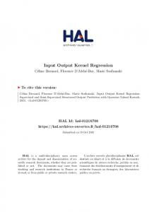
Practical Results epsilon-bound
Weight Vector Minimisation 360
340
risky
conservative
340
320
risky
320
conservative
280
Q-Value
Q-Value
300 300
280
260 260 240
220
240
0
2
4
6
8
10
12
Position
14
16
18
20
220
0
2
4
6
8
10
12
Position
14
16
18
20
Fig. 1: Impacts of different regularisers on the Wet-Chicken Q-function. Solid line: Ridge Regression only, Dashed: with accordant regularisation. At the intersections of the Q-function the action each changes. The closer the intersection point lies to the waterfall (right), the riskier is the policy. To show, how EKRR and their different regularisation extensions work, we applied the method on the so-called Wet-Chicken problem [12]. It is a quite simple, but probabilistic benchmark RL task. The only dimension of the state space represents a river on which a canoeist has to paddle. On the end there is a waterfall and the task is to come as close as possible to the waterfall without falling down. Otherwise the canoeist has to restart. The reward increases linearly with the proximity to the waterfall. Simulated turbulences make the state transition probabilistic. We modeled two different actions: drifting downstream and rowing upstream. The canoeist has to force back as late as possible and as early as necessary. In fig. 1 we opposed standard EKRR and EKRR with different regularisation settings: minimising the weight vector and tolerating an �-tube. The two regularisation methods result in more conservative policies. As expected, the regularisation sanctions have smoothing effects and lead to a bias to a simpler function class.
341
ESANN'2007 proceedings - European Symposium on Artificial Neural Networks Bruges (Belgium), 25-27 April 2007, d-side publi., ISBN 2-930307-07-2.
6
Conclusion
Kernel Rewards Regression was developed to handle Optimal Control problems data-efficiently. But as many RL methods, it has to deal with a kind of Policy Iteration to achieve a near-optimal policy. To avoid these iteration schemes and eventual convergence problems, Explicit Kernel Rewards Regression proposes the possibility to identify a near-optimal policy directly by applying just one quadratic program. Hence, solving the RL problem becomes a task of well-known numerical methodologies [13, 14] for non-linear and non-convex optimisation. Furthermore, several regularisation techniques, known from Statistical Learning Theory, can be easily applied. They trade between different policy properties. On a given benchmark, we showed that certain regularisation techniques control the policies’ riskiness, their certainty, and the complexity of the Q-function.
7
Acknowledgment
The authors would like to thank Michael Metzger for very helpful hints formulating the Optimal Control problem as quadratic program.
References [1] Richard S. Sutton and Andrew G. Barto. Reinforcement Learning: An Introduction. MIT Press, Cambridge, 1998. [2] Richard S. Sutton, Andrew G. Barto, and Ronald J. Williams. Reinforcement learning is direct adaptive optimal control. IEEE Control Systems Magazine, 12:19–22, 1992. [3] Richard S. Sutton. Open theoretical questions in reinforcement learning. In EuroCOLT, pages 11–17, 1999. [4] Michael G. Lagoudakis and Ronald Parr. Least-squares policy iteration. Journal of Machine Learning Research, pages 1107–1149, 2003. [5] Yaakov Engel, Shie Mannor, and Ron Meir. Bayes meets bellman: The gaussian process approach to temporal difference learning. In Proc. of ICML, pages 154–161, 2003. [6] Martin Riedmiller. Neural fitted q-iteration - first experiences with a data efficient neural reinforcement learning method. In Proceedings of the 16th European Conference on Machine Learning, pages 317–328, 2005. [7] D. Ormoneit and S. Sen. Kernel-based reinforcement learning. Machine Learning, 49(23):161–178, 2002. [8] T. Dietterich and X. Wang. Batch value function approximation via support vectors. In NIPS, pages 1491–1498, 2001. [9] Daniel Schneegass, Steffen Udluft, and Thomas Martinetz. Kernel rewards regression: An information efficient batch policy iteration approach. In Proc. of the IASTED Conference on Artificial Intelligence and Applications, pages 428–433, 2006. [10] Nello Cristianini and John Shawe-Taylor. Support Vector Machines And Other Kernelbased Learning Methods. Cambridge University Press, Cambridge, 2000. [11] Daniel Schneegass. Structural risk minimisation for data-efficient reinforcement learning. Siemens AG, CT IC 4, Technical Report, 2006. [12] Volker Tresp. The wet game of chicken. Siemens AG, CT IC 4, Technical Report, 1994. [13] L.E.Scales. Introduction to non-linear optimization. Springer-Verlag, New York, 1985. [14] R. Byrd, J. C. Gilbert, and J. Nocedal. A trust region method based on interior point techniques for nonlinear programming. Mathematical Programming, 89(1):149–185, 2000.
342