EXPLICIT SEGMENTATION OF SPEECH FOR ... - MILE Lab - IISc

EXPLICIT SEGMENTATION OF SPEECH FOR INDIAN LANGUAGES

A Thesis Submitted for the Degree of

Master of Science in the Faculty of Engineering

By

Ranjani H G

Department of Electrical Enginnering

Indian Institute of Science Bangalore - 560 012 India March 2008

Acknowledgements A journey is never difficult when you travel together. Interdependency is more fruitful and valuable than independence. This thesis is a result of two and a half years of creativity, hard work and support provided to me by all those near and dear to me. I take this opportunity to express my gratitude. The first person I would like to thank is Prof. Dr. A G Ramakrishnan my mentor and my direct supervisor . I have been under his guidance from 2005 when I started my Masters of Science in IISc. During these years, I have known him as a empathetic listener, principle oriented professor and a humble human being. I learnt the importance of ‘quality work’ from him. I cannot thank him enough for his encouragement and his accommodative nature to tolerate my presence and absence. I would also like to thank Prof. K R Ramakrishnan, Prof. T V Sreenivas, Prof. K V S Hari, Prof. Srikanth Iyer and Prof. P S Sastry - my professors who taught me. They made the courses they taught so interesting. I have had the pleasure to work with my lab mate G Ananthakrishnan. The motivation he provided me throughout my research helped me overcome so many obstacles and frustrations to finally get my results. Many a thanks to him. Prof. T V Ananthapadmanabha gave me a lot of suggestions during the latter part of my research work. The discussions I had with him provided me with valuable ideas and helped me to successfully complete my thesis work. I am overjoyed to get his feedbacks. I thank him for all his help.

Acknowledgements

ii

Also, I take pride in the support provided to me by my great friends - Krishnaveni, Santhosh, my (ex)roomie Preethi and Lakshmish - for listening to my concerns, tales of difficult times and joyous moments during my research. I thank them for being with me when I needed them the most. My life in IISc would not have been the same without my labmates - Thot, Suresh, Neelam, Srilakshmi, Bhavna, Jayant, Kiran, Ravishanker, Manju, Aditya, Sharanya, Vani, Shashi, Kandan, Shanthi, Seema & Nirup. I thank them for the memories of fun times I had with them. These memoirs are gifts that will always bring a smile to my face. Special thanks to Srilakshmi, Shanthi, Jayant, Suresh and Seema for all the support they gave during my thesis phase of research. I also thank my classmates - Srikanth, Krusheel, Ranjith, Partha and Paresh - for the exciting discussions we had during our class work. I feel a deep sense of gratitude towards my parents, my source, who have sculpted me to what I am today. They taught me all the good things in life and inculcated in me the values which have helped me sail through the most difficult times. I would like to acknowledge the tremendous sacrifices they made to ensure that I had an excellent education. I am ever so grateful to my brother, my sister and brother-in-law for all their encouragement and support - they had more faith in me than could ever be justified by logical argument. I cannot thank my husband, Ajey, enough for being my pillar of support and unconditional love throughout this journey. Without him, I would have struggled to find the inspiration and motivation needed to complete this work. I am among the lucky few who get a wonderful couple as in-laws - they were very encouraging, supportive and accommodative throughout my masters degree. It is difficult to overstate my gratitude towards them. My loving thanks to Lakshmi. I enjoyed the company and support of many others whom I fail to mention here, and I’m thankful for your help and friendship.

Acknowledgements

iii

Above all, I want to thank my little angel, my daughter - Shaarada whose innocent face and pranks made me forget my dejections and helped me overcome my failures in a graceful way. She has given me the greatest gift of being a mother. Last but not the least, thanks to God for all the tests in life thus making my life more bountiful. May His name be exalted, honored, and glorified.

I dedicate this thesis to my angel Shaarada.

Abstract Speech segmentation is the process of identifying the boundaries between words, syllables or phones in the recorded waveforms of spoken natural languages. The lowest level of speech segmentation is the breakup and classification of the sound signal into a string of phones. The difficulty of this problem is compounded by the phenomenon of co-articulation of speech sounds. The classical solution to this problem is to manually label and segment spectrograms. In the first step of this two step process, a trained person listens to a speech signal, recognizes the word and phone sequence, and roughly determines the position of each phonetic boundary. The second step involves examining several features of the speech signal to place a boundary mark at the point where these features best satisfy a certain set of conditions specific for that kind of phonetic boundary. Manual segmentation of speech into phones is a highly time-consuming and painstaking process. Required for a variety of applications, such as acoustic analysis, or building speech synthesis databases for high-quality speech output systems, the time required to carry out this process for even relatively small speech databases can rapidly accumulate to prohibitive levels. This calls for automating the segmentation process. The state-of-art segmentation techniques use Hidden Markov Models (HMM) for phone states. They give an average accuracy of over 95% within 20 ms of manually obtained boundaries. However, HMM based methods require large training data for good performance. Another major disadvantage of such speech recognition based segmentation techniques is that they cannot handle very long utterances, which are

Abstract

vi

necessary for prosody modeling in speech synthesis applications. Development of Text to Speech (TTS) systems in Indian languages has been difficult till date owing to the non-availability of sizeable segmented speech databases of good quality. Further, no prosody models exist for most of the Indian languages. Therefore, long utterances (at the paragraph level and monologues) have been recorded, as part of this work, for creating the databases. This thesis aims at automating segmentation of very long speech sentences recorded for the application of corpus-based TTS synthesis for multiple Indian languages. In this explicit segmentation problem, we need to force align boundaries in any utterance from its known phonetic transcription. The major disadvantage of forcing boundary alignments on the entire speech waveform of a long utterance is the accumulation of boundary errors. To overcome this, we force boundaries between 2 known phones (here, 2 successive stop consonants are chosen) at a time. Here, the approach used is silence detection as a marker for stop consonants. This method gives around 89% (for Hindi database) accuracy and is language independent and training free. These stop consonants act as anchor points for the next stage. Two methods for explicit segmentation have been proposed. Both the methods rely on the accuracy of the above stop consonant detection stage. Another common stage is the recently proposed implicit method which uses Bach scale filter bank to obtain the feature vectors. The Euclidean Distance of the Mean of the Logarithm (EDML) of these feature vectors shows peaks at the point where the spectrum changes. The method performs with an accuracy of 87% within 20 ms of manually obtained boundaries and also achieves a low deletion and insertion rate of 3.2% and 21.4% respectively, for 100 sentences of Hindi database. The first method is a three stage approach. The first is the stop consonant detection stage followed by the next, which uses Quatieri’s sinusoidal model to classify sounds as voiced/unvoiced within 2 successive stop consonants. The final stage uses

Abstract

vii

the EDML function of Bach scale feature vectors to further obtain boundaries within the voiced and unvoiced regions. It gives a Frame Error Rate (FER) of 26.1% for Hindi database. The second method proposed uses duration statistics of the phones of the language. It again uses the EDML function of Bach scale filter bank to obtain the peaks at the phone transitions and uses the duration statistics to assign probability to each peak being a boundary. In this method, the FER performance improves to 22.8% for the Hindi database. Both the methods are equally promising for the fact that they give low frame error rates. Results show that the second method outperforms the first, because it incorporates the knowledge of durations. For the proposed approaches to be useful, manual interventions are required at the output of each stage. However, this intervention is less tedious and reduces the time taken to segment each sentence by around 60% as compared to the time taken for manual segmentation. The approaches have been successfully tested on 3 different languages, 100 sentences each - Kannada, Tamil and English (we have used TIMIT database for validating the algorithms). In conclusion, a practical solution to the segmentation problem is proposed. Also, the algorithm being training free, language independent (ES-SABSF method) and speaker independent makes it useful in developing TTS systems for multiple languages reducing the segmentation overhead. This method is currently being used in the lab for segmenting long Kannada utterances, spoken by reading a set of 1115 phonetically rich sentences.

Contents

Acknowledgements

i

Abstract

v

List of Figures

xiii

List of Tables

xv

1 Introduction

1

1.1

Literature survey of implicit methods . . . . . . . . . . . . . . . . . .

5

1.2

Literature survey of explicit methods . . . . . . . . . . . . . . . . . .

7

1.3

Literature survey on segmentation for Indian languages . . . . . . . .

8

2 Stop-consonant detection

11

2.1

The stop-consonants . . . . . . . . . . . . . . . . . . . . . . . . . . . 12

2.2

Detection of stop consonants . . . . . . . . . . . . . . . . . . . . . . . 15

2.3

Results and analysis . . . . . . . . . . . . . . . . . . . . . . . . . . . 16

CONTENTS

ix

3 The Bach scale filter bank

23

3.1

The Bach scale filter bank . . . . . . . . . . . . . . . . . . . . . . . . 23

3.2

Obtaining the feature vectors . . . . . . . . . . . . . . . . . . . . . . 27

3.3

Two class problem . . . . . . . . . . . . . . . . . . . . . . . . . . . . 27

3.4

Distance functions . . . . . . . . . . . . . . . . . . . . . . . . . . . . 28

3.5

Comparative analysis. . . . . . . . . . . . . . . . . . . . . . . . . . . 29

4 ES-SABSF method 4.1

32

Sinusoidal model for speech . . . . . . . . . . . . . . . . . . . . . . . 32 4.1.1

Segmentation into voiced and unvoiced regions . . . . . . . . . 35

4.2

The ES-SABSF algorithm . . . . . . . . . . . . . . . . . . . . . . . . 36

4.3

Results and discussion . . . . . . . . . . . . . . . . . . . . . . . . . . 38

5 ES-DSBSF method

50

5.1

The proposed algorithm . . . . . . . . . . . . . . . . . . . . . . . . . 50

5.2

Results and discussion . . . . . . . . . . . . . . . . . . . . . . . . . . 53

6 Conclusions and future work

60

A Appendix

62

References

66

List of Figures

1.1

Manual segmentation using temporal and spectral changes . . . . . .

4

2.1

Classification of stops in Sanskrit language . . . . . . . . . . . . . . . 15

2.2

Magnitude and phase response of the high-pass Bessel filter . . . . . . 16

2.3

Stop consonants before and after high-pass filtering . . . . . . . . . . 17

2.4

Performance of the stop detection algorithm for various values of µ (minimum number of consecutive frames.) . . . . . . . . . . . . . . . 18

2.5

The effect of the order of the Bessel filter on the performance of the stop detection algorithm. . . . . . . . . . . . . . . . . . . . . . . . . . 19

2.6

An instance of stop consonant that cannot be detected . . . . . . . . 21

3.1

The Bach scale . . . . . . . . . . . . . . . . . . . . . . . . . . . . . . 24

3.2

The log magnitude responses of the filters of the Bach scale for nonlinear and linear formulations . . . . . . . . . . . . . . . . . . . . . . 26

3.3

The comparison of the bandwidths of different scales . . . . . . . . . 26

LIST OF FIGURES

xi

4.1

Sinusoidal analysis of speech . . . . . . . . . . . . . . . . . . . . . . . 35

4.2

Block diagram of the proposed ES-SABSF algorithm. . . . . . . . . . 37

4.3

Sinusoidal analysis for an utterance in Hindi. . . . . . . . . . . . . . . 38

4.4

Segmenting for multiple boundaries within a voiced region using EDML function - Hindi . . . . . . . . . . . . . . . . . . . . . . . . . . . . . 39

4.5

A segment of speech waveform from Hindi database with its automated and manually detected boundaries. . . . . . . . . . . . . . . . 40

4.6

Sinusoidal analysis for an utterance from TIMIT database . . . . . . 40

4.7

Segmenting for multiple boundaries within the voiced regions using EDML function - English . . . . . . . . . . . . . . . . . . . . . . . . . 41

4.8

Speech waveform from TIMIT database with manual and automated boundaries . . . . . . . . . . . . . . . . . . . . . . . . . . . . . . . . . 42

4.9

Sinusoidal analysis for an utterance from Tamil database. . . . . . . . 43

4.10 Segmenting for multiple boundaries within the voiced regions using EDML function - Tamil . . . . . . . . . . . . . . . . . . . . . . . . . 44 4.11 Speech waveform from Tamil database with manual and automated boundaries . . . . . . . . . . . . . . . . . . . . . . . . . . . . . . . . . 45 4.12 Sinusoidal analysis for an utterance from Kannada database. . . . . . 45 4.13 Segmenting for multiple boundaries within the voiced regions using EDML function - Kannada . . . . . . . . . . . . . . . . . . . . . . . . 46 4.14 Speech waveform from Kannada database with manual and automated boundaries . . . . . . . . . . . . . . . . . . . . . . . . . . . . . 47

LIST OF FIGURES

xii

4.15 Sinusoidal analysis for an utterance from Hindi database - example 2

47

4.16 Segmenting for multiple boundaries within the voiced regions using EDML function - Hindi - example 2 . . . . . . . . . . . . . . . . . . . 48 4.17 Speech waveform from Hindi database with manual and automated boundaries . . . . . . . . . . . . . . . . . . . . . . . . . . . . . . . . . 49

5.1

A portion of Hindi speech utterance between a silence and a stop region 51

5.2

EDML function of the speech waveform between β1 and β2 - Hindi . . 52

5.3

Nodes with transition probabilities. . . . . . . . . . . . . . . . . . . . 53

5.4

Speech waveform from the Hindi database with manually and automatically detected boundaries . . . . . . . . . . . . . . . . . . . . . . 54

5.5

The portion of English utterance between 2 silence regions from the TIMIT database . . . . . . . . . . . . . . . . . . . . . . . . . . . . . 54

5.6

EDML function of the speech waveform between β1 and β2 - English . 55

5.7

Speech waveform from TIMIT database with manual and automated boundaries . . . . . . . . . . . . . . . . . . . . . . . . . . . . . . . . . 56

5.8

A portion of a Tamil utterance between 2 stop regions . . . . . . . . 56

5.9

EDML function of the speech waveform between β1 and β2 - Tamil . 57

5.10 Speech waveform from Tamil database with manual and automated boundaries . . . . . . . . . . . . . . . . . . . . . . . . . . . . . . . . . 58 5.11 A portion of Kannada speech utterance between 2 stop regions

. . . 58

5.12 EDML function of the speech waveform between β1 and β2 - Kannada 59

LIST OF FIGURES

xiii

5.13 Speech waveform from Kannada database with manual and automated boundaries . . . . . . . . . . . . . . . . . . . . . . . . . . . . . 59

A.1 Segmentation using EDM, EDML and NEDML distance functions.

. 65

List of Tables

2.1

Performance comparison of detection of stop consonants in the TIMIT database - Algorithms in the literature v/s proposed algorithm. . . . 19

2.2

Performance of the proposed stop consonant detection algorithm for various languages . . . . . . . . . . . . . . . . . . . . . . . . . . . . . 20

3.1

Performance of the stop consonant detection algorithm using MFCC and BFCC for various languages . . . . . . . . . . . . . . . . . . . . . 30

4.1

Comparison of performance of sinusoidal model for different languages 36

4.2

Comparison of segmentation performances on TIMIT database: Algorithms in the literature vs ES-SABSF. . . . . . . . . . . . . . . . . 39

4.3

Frame Error Rate (FER) between successive stop consonants of the proposed ES-SABSF method for different languages. . . . . . . . . . . 42

5.1

Frame Error Rate(FER) between 2 successive stop consonants for the proposed ES-DSBSF method for different languages. . . . . . . . . . 55

A.1 Segmentation performance of various methods on the TIMIT database. 63

LIST OF TABLES

xv

A.2 Comparison of segmentation performances of various filter-banks on TIMIT database. . . . . . . . . . . . . . . . . . . . . . . . . . . . . . 64 A.3 Comparison between the performances of various distance functions in segmenting the Hindi database. . . . . . . . . . . . . . . . . . . . . 64 A.4 Comparison of the segmentation performance of EDML using Bach Linear filter-bank for various languages. . . . . . . . . . . . . . . . . . 64

Chapter 1 Introduction Of course, this fragmentation is not unique to research in the field of spoken language processing. Since Descartes, scientific reductionism has dominated as the main paradigm for understanding natural phenomena. For over 400 years, scientists have made tremendous progress across the breadth of human knowledge by making assumptions and approximations in order to partition a problem into more easily addressable sub-parts. However, the downside of the standard scientific method is that it leads inevitably to greater and greater knowledge about smaller and smaller aspects of a problem. As a result, progress towards the unification of different theories can be slow and ponderous, and success on the scientific grand challenges continues to elude the scientific community [1].

Speech segmentation is the determination of the beginning and ending boundaries of acoustic units. Generally, segmentation is divided into two levels:

• Lexical segmentation: Decomposition of spoken language into smaller lexical segments such as paragraphs, sentences, phrases, words and syllables. • Phonemic segmentation: Segmentation and classification of the sound signal at the lowest level to a string of acoustic elements (phones), which

Introduction

2

represent distinct target configurations of the speech tract (w.r.t. articulation as well as form of excitation). Speech segmentation at the phone level refers to the process of getting accurate time markers indicating the beginning and ending of phones in a spoken sentence. Many speech processing problems usually require segmenting the speech corpora into phonemic units and also labeling them. Usually, the goal is to save or process these units or to reduce the quantity of information to code. When dealing with speech transmission, segmentation is used to locate the stationary segments over which the signal can be modeled with a unique timeinvariant model. This allows for the increase of the average estimation interval, which in turn enables the reduction of the baud rate required to maintain the high quality transmission [2]. The analysis of speech sounds in different contexts requires a tedious work of collecting samples of the sounds because of which speech segmentation becomes important in speech recognizers. Although actual techniques do not require an explicit segmentation, it is accepted that faster training and better results are achieved if the modeling techniques are initialized with some segmentation of the speech. This is specially important for the methods which require time consuming procedures for training. Furthermore, the labels are used to evaluate recognition systems. The performance of the systems is usually measured by aligning the recognized transcription with the reference transcription [3]. Finally, segmentation of speech is also important in speech synthesis. Here, a large number of units need to be segmented to build a dictionary of sub-word units. This thesis attempts to automate this process. A high quality unit selection speech synthesizer requires the recording of proper data. Although a number of studies have investigated what data is correct for a particular domain [4, 5], typical recorded databases only have isolated sentences, and this appears insufficient for constructing natural and consistent prosody above the sentence level. It is required to record from a single speaker, utterances of a

Introduction

3

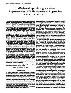
paragraph and longer monologues, which cover various phonetic-acoustic contexts. To use such databases for the construction of a unit selection synthesizer, it is necessary to segment and label the positions of the units. In speech synthesis, segmentation and annotation of the speech at the phonemic level has become a standard requirement. The synthesis block of the Text-to-Speech (TTS) systems concatenates the phone units (present in the inventory) based on the left and right contexts. The quality of segmentation is crucial because an error in segmentation results in an audible error in the synthesized speech. However, boundary errors of the order of 20-30 ms are not audible and are considered acceptable. Segmentation, from now on, refers to speech segmentation at phone level, unless otherwise mentioned. The difficulty of this segmentation problem is compounded because of the phenomenon of co-articulation of speech sounds, where it may be modified in various ways by the adjacent ones such as blending smoothly, fusing, splitting, or at times even disappearing. This phenomenon may happen between adjacent words just as easily as within a single word. Whether ‘true’ phone boundaries do exist is subject to discussion. Therefore the term correct phone boundaries, here, refer to locations in time-domain, which are marked by human experts based on prominent acoustic events such as sudden changes in speech spectra or energy [6]. Hence, the classical solution to this (segmentation) problem is to manually label and segment spectrograms. The process of manual labeling and segmenting of speech can be seen as a two-step process. In the first step, a trained person listens to a speech signal, recognizes the word and phoneme sequence, and roughly determines the position of each phonetic boundary. The second step involves examining several speech signal features (waveform, energy, spectrogram etc.,) to place a phonetic boundary time mark, where these features best satisfy a certain set of conditions specific for that kind of phonetic boundary [7]. The changes in spectral and temporal characteristics used to segment the phones in a speech waveform can be seen in Fig. 1.1. Manual labeling and segmentation, though reliable, has two disadvantages. First,

Introduction

4

it is very time consuming as manual labeling of a single utterance can take several hours. The cost of establishing a sizeable acoustic phonetic database is therefore high. More is the difficulty of generating reproducible results. Informal comparisons during the establishment of an acoustic-phonetic database of continuous speech shows the near impossibility of two researchers obtaining identical segmentation results even though a strategy is laid down in fine detail. A rough segmentation at the syllable level might be consistent. However, the finer segmentation remains arbitrary to a certain extent especially where several phones fall into one syllable without exhibiting any discontinuities of the parameter functions or their derivatives. The need for a large-scale acoustic-phonetic database and the concern about the validity of the speech analysis performed on such a database call for the development of automatic segmentation and labeling [8]. There are 2 types of automated segmentation: Implicit segmentation or blind segmentation does not have any priori knowledge of the phonetic transcription. Whereas, the problem of finding phonetic boundaries of a text given its phonetic content is known in the literature as linguistically constrained seg-

Figure 1.1: Manual Segmentation using temporal and spectral changes for the Kannada utterance - ‘SwasochAsadasangkyEkaDim’ using Praat software

Introduction

5

mentation or explicit segmentation. Implicit segmentation methods result in ‘deletions’ and ‘insertions’. Absence of an automated boundary within 20 ms of a manual boundary results in deleted boundary. When there is more than one automated boundary within 20 ms of a manual boundary or an automated boundary where there is no manual boundary, it is an inserted boundary.

1.1

Literature survey of implicit methods

The earliest attempts at automated segmentation were achieved using the spectrogram of the signal and counting the number of zero-crossings in a region of speech [9, 10]. Van Hemert used the intra frame correlation measure [11] between spectral features to obtain the segments. Though the method resulted in 91% accuracy, the experiments were on isolated words and not on continuous speech. Statistical modeling (AR, ARMA) [12] has also been used. It is based on Brandt’s model that every homogeneous segment of the signal is described by an AR model of order p, and hence a jump in the AR coefficients and variance of the residue corresponds to an event in speech signal. The most popularly used methods are the Spectral Transition Measure (STM) and the Maximum Likelihood (ML) segmentation methods [14]. STM method uses the fact that at the times when the vocal tract changes rapidly, as at the boundaries between different speech sounds, the magnitude of the derivative of the vector (representing spectral features) peaks. However, this method requires a threshold for peak picking. ML method is conditioned on the criteria that the acoustic inhomogeneity of a

Introduction

6

segment needs to be minimized. This inhomogeneity is seen as the intra-segmental distortion i.e., distortion from the frames that span the segment to the centroid of the segment. The centroid of a segment is viewed as the ML estimate of the frames in the segment. ML segmentation method uses the dynamic programming algorithm and is terminated when the distortion falls below a specified threshold. Alternatively, the method can also be input with the number of segments required (explicit method). Another method which uses average level-crossing rate (A-LCR) has been suggested by Sarkar [15]. This method explores detecting signal changes with a view that temporal features are more reliable than the standard feature domain methods, since both magnitude and phase information are retained. It uses the A-LCR to detect significant temporal changes in the signal. The method outperforms STM and doesn’t use the information of number of segments unlike STM and ML methods. Nagarajan, Murthy and Hegde [16] have used group delay functions to segment speech into syllable-like units. Three different minimum phase signals are derived from the short term energy functions of three sub-bands of the speech signal, as if it were a magnitude spectrum. Boundaries are defined by combining the peaks of the group delay functions of each of these three sub-bands. All the above cited methods do not need training and are implicit segmentation methods. However, ML and STM methods can be modified to take into account the number of segment boundaries required. In automating the segmentation process for TTS corpora, a forced alignment system can be used. The uttered word sequence is known in advance and the phonetic transcription of the recordings can be derived from the orthographic text using a grapheme to phoneme (G2P) converter. Thus, the task of the system is to find the best alignment of the transcription sequence to the speech signal. This is an explicit segmentation problem. Although in few cases, the utterance may deviate from its phonetic transcription, mainly due to dialectal variations, this problem is not dealt with in this work. It

Introduction

7

is assumed that the utterance corresponds to the phonetic transcription obtained from G2P.

1.2

Literature survey of explicit methods

The most successful segmentation methods have been borrowed from automatic speech recognition, such as Hidden Markov Models (HMM) [17] or Dynamic Time Warping (DTW) [18], because automatic alignment can be viewed as a simplified recognition task. In a HMM based segmentation technique, the HMM recognizer is used to do forced alignment. A known sequence of phoneme models is used with the Viterbi algorithm to generate a phonetic alignment giving an accuracy of around 79%. Context independent HMMs perform better than the context dependent HMMs. However, an initial estimate of the labeling is generated using a context dependent phone based HMM (CDHMM) [13, 19]. Finer refinement of boundaries is achieved by parsing through the sentence a second time. This refinement has been proposed using various techniques: Fuzzy logic, neural networks, Gaussian mixture models (GMMs) or Multi-layer perceptron (MLP) [20] with boundary accuracies of 94%, 96%, 94% and 94% within 20 ms of manually determined boundaries. Further, the accuracy increases to 99% when speaker adaptation techniques are used. On the other hand, if DTW were used, the signal is aligned with some kind of known reference containing the expected segments. In the above methods, the boundaries are inferred from the recognition results, which are not necessarily consistent with the correct phone boundaries. This might not significantly affect the recognition accuracies of speech recognizers, but deviations from prominent acoustic events affect the performance of speech processing algorithms heavily relying on precise phone boundary detections [21]. Also, these techniques do not appear to work that well on databases with longer utterances that are required for better super-sentential prosodic modeling [22]. Hence, these techniques also require a manual correction of boundaries. Also, they are data dependent

Introduction

8

- larger the training data, better is the performance of training based segmentation methods.

1.3

Literature survey on segmentation for Indian languages

A survey of segmentation techniques in the literature for Indian languages show techniques segmenting Tamil and Telugu databases at syllable level explored by Hema Murthy [16, 23, 24]. Subspace based segmentation at CV level was proposed by Muralishankar and Vijayakrishna [25] for Kannada and Tamil languages. Prahallad [26] proposes segmentation using neural networks on Hindi database with a reported accuracy of 95%. Ananthakrishnan [27, 28] proposed a filter bank approach for training-free, implicit segmentation at phone level (language independent), which gave good segmentation accuracy for Indian languages. However, literature available dealing with segmentation of speech at phone level for Indian languages is limited. The scenario for Indian languages is such that large standard databases are not available for training. Also, little literature is available for modeling prosody in Indian languages [30, 31, 32]. Research in this area is very recent [33]. Therefore, we have recorded long utterances at the paragraph level and monologues for creating the databases. Typically, sentences have an average of 170 phones and some sentences even extend to more than 1000 phones. Alignment of the text to recorded speech is limited by the fact that standard techniques do not handle such very long utterances well. Recently, Prahallad [34] discusses ways to handle issues in processing of large multi-paragraph speech databases that can be used in speech synthesis. The aim of this thesis is to automate the process of aligning a given sequence of phones for long spoken utterances recorded for the purpose of development of TTS application. Instead of attempting to segment the long utterances at once, segmenting it

Introduction

9

within smaller regions leads to better accuracy of segmentation. Here, we attempt to detect stop consonants and use them as anchor points for the next stage. Two methods have been proposed for force aligning of boundaries. Both methods rely on the accuracy of the above stop consonant detection stage. Another common stage of both the algorithms is the use of Bach scale filter bank to obtain the feature vectors. A distance function of these feature vectors shows peaks at the points, where the spectrum significantly changes [27, 28]. The first method is a multi-stage approach, which combines 3 algorithms. The first is the stop consonant detection stage. The next stage uses Quatieri’s sinusoidal model [42] to classify sounds within 2 successive stop consonants as voiced/unvoiced. The final stage uses the distance function of feature vectors of Bach scale filter bank to further obtain boundaries within the voiced and unvoiced regions. In this work, this method will be referred to as ‘Explicit Segmentation using Sinusoidal Analysis and Bach Scale Filter-banks’ (ES-SABSF). The second method uses duration statistics of the phonemes of the language. It again uses the distance function of Bach feature vectors (i.e., feature vectors obtained from Bach scale filter banks) to obtain peaks at the phone transitions and uses the duration statistics to assign probability to a particular peak being a boundary. In this thesis, this method will be referred to as ‘Explicit Segmentation using Duration Statistics and Bach Scale Filter-bank’ (ES-DSBSF). Both the methods are equally promising for the fact that they give low frame error rates as compared to those proposed in the literature. However, results show that the second method (ES-DSBSF) outperforms the first (ES-SABSF), because it incorporates the knowledge of durations. For the two proposed segmentation approaches to be useful, manual interventions are required at the output of stop detection stage and the final stage. However, these interventions are less tedious. In conclusion, we have proposed a practical solution to the segmentation prob-

Introduction

10

lem. The proposed methods reduce the time taken to segment each sentence by around 60% as compared to the time taken for manual segmentation. Being training free, language independent (method 1) and speaker independent, the algorithm facilitates development of TTS systems for multiple languages with reduced segmentation overhead. The outline of the thesis is as follows : The detection of stop consonants is dealt with in Chapter 2. Chapter 3 summarizes the implicit segmentation technique using Bach scale filter bank. Chapters 4 and 5 describe the ES-SABSF and ES-DSBSF methods, respectively along with a discussion on their performance. Chapter 6 concludes the thesis.

Chapter 2 Stop-consonant detection The major disadvantage of forcing boundary alignments on long utterances is that an error in detecting one of the segment boundary can result in error in subsequent boundaries. To circumvent this drawback, we propose to force boundaries between 2 known phones, so that the boundary error occurring at the start of the speech waveform does not propagate to the end. We can identify a phoneme class in either of the two ways : • Using a phoneme/ phoneme class recognition system • Using a phoneme/ phoneme class detection system. A recognition system will invariably lead to a system that requires training. However, our motivation is to segment speech with no training. Hence, a simple phoneme class detection algorithm can be used. The phonemes can be broadly classified into the following classes: • Fricatives • Vowels

Stop-consonant detection

12

• Nasals • Nasalized vowels • Diphthongs • Glides • Stop consonants • Silence Fricatives, vowels, nasals, diphthongs, nasal vowels and glides need some stored form of features to be able to detect them. Also, different phonemes in each class require different features. However, stop consonants can be efficiently detected without storing any features. Hence, we choose to detect all the stop consonants in the utterance as the first step and this is described in this chapter.

2.1

The stop-consonants

A stop or plosive or occlusive is a consonant produced by stopping the airflow in the vocal tract. All languages of the world have stops (some Polynesian languages have only three). Most languages have at least [p], [t], [k], [n], [m]. In the articulation of a stop consonant, three phases can be distinguished: • Catch or occlusion : The airway closes so that no air can escape through the mouth; hence the name occlusive. With nasal stops, the air escapes through the nose. • Hold or stop: The airway stays closed causing a pressure difference to build up; hence the name, stop. • Release, burst or plosive: The closure is opened. In the case of plosives, the released airflow produces a sudden impulse, causing an audible sound; hence the name plosive.


13

In certain languages, some stops may lack the final release. These are called unreleased stops. (Example. In English, [p] in ‘apt’ and [n] in ‘ant’ are unreleased stops.)

Based on the manner and place of articulation, stop consonants can be broadly classified as:

• Nasal or oral stops: If the velum is lowered, thus allowing air to escape through the nose during the production of the stop, then it is a nasal stop. Else it is an oral stop. • Voiced or unvoiced stops: Voiced stops are articulated with simultaneous vibration of the vocal cords, while unvoiced stops are articulated without vibration of cords. • Aspirated or unaspirated stops: In aspirated stops, there is a strong frication noise after release, whereas unaspirated stops have no frication after release. Most Indian languages have separate phonemes for aspirated stops. • Short or long stops: In a long stop, the second phase of the articulation of the stop takes more time than a short stop. Typically, long stops take about three times the closure duration of the short ones.

Stops may be made with more than one airstream mechanism:

• Pulmonic egressive: This is the normal mechanism, where the air flowing outward is powered by the lungs (actually, the ribs and diaphragm). All languages have pulmonic stops. • Ejectives or glottalic egressive: In this mechanism, the airstream is powered by an upward movement of the glottis rather than by the lungs or diaphragm. Plosives, affricates and occasionally, fricatives may occur as ejectives. All ejectives are unvoiced.


14

• Implosives or glottalic ingressive: Here, the glottis moves downward, but the lungs may be used simultaneously to provide voicing, and in some languages no air may actually flow into the mouth. The vast majority of implosive consonants are voiced and they are frequent among African languages. • Clicks: These are stops produced with two articulatory closures in the oral cavity. The two closures involved are : an anterior one which is regarded as primary and determines the click’s place of articulation, and a posterior one which can be oral or nasal, voiced or voiceless. The classification of stop consonant sounds based on manner of articulation results in a stop sound containing 2 to 4 of the following events: • Closure duration, which is mostly silent. • Release with clearly marked noise burst. • Frication after burst release for aspirated stops. • Voice Onset Time, (VOT), which is the length of time that passes between the release of the consonant and the beginning of the vibration of the vocal folds. VOT is near zero for unvoiced stops, negative for voiced stops and positive for aspirated stops. These events are also called ‘micro-phonetic segments’ with respect to stop consonants. Most of the Indian languages have evolved from Sanskrit. Fig. 2.1 shows the traditional listing of the Sanskrit consonants with the (nearest) equivalents in English or Spanish. Each consonant shown is deemed to be followed by the neutral vowel schwa (/a/), and is named as such below [35]. Except the nasal plosives, we classify the rest of the combinations of voiced or unvoiced, aspirated or unaspirated plosives in any Indian language in the stop consonant class.


15

Figure 2.1: Classification of stops in Sanskrit language: Along the rows is the manner of articulation and along the columns is the place of articulation.

2.2

Detection of stop consonants

The algorithm proposes to detect silence as a marker for stop consonants. It can be noted that every stop consonant has the silence as the cue for the closure region. However, voiced stop consonants have a low frequency signal in the closure region. To remove this low frequency signal, the speech signal is high pass filtered with a Bessel filter, whose cutoff frequency is 400 Hz. The magnitude and phase responses of the Bessel filter are shown in Fig. 2.2. A voiced stop consonant, before and after high pass filtering is shown in Fig. 2.3(a) and (b) respectively. The first few frames (considering a frame to be 10 ms long) of any spoken sentence is predominantly silence. Now, the MFCCs of all the frames of the filtered speech


16

are calculated. The Euclidean distance is computed between the MFCC of first frame and MFCC of every other frame. If this distance drops below a threshold value for a minimum of µ consecutive frames, then the algorithm decides that the corresponding region may contain the silence part of a stop consonant or a silent interval in speech or a combination of both. The frame within this region having the minimum distance from the first silence frame is surely a stop consonant (or silence or both) frame. Fig. 2.3(c) shows the output of the algorithm for the waveform in Fig. 2.3(a).

2.3

Results and analysis

If an output frame from the stop detection algorithm is well within the stop region/ silence region, then the first sample of that particular frame is an accurate output. If there is more than one output within a single stop region/ silence region, or if there Magnitude (dB) and Phase Responses 0

−100 Filter #1: Magnitude Filter #1: Phase

−50

−240

−100

−380

−150

−520

−200

−660

−250 0

Phase (degrees)

Magnitude (dB)

Normalized Frequency: 0.05004883 Magnitude (dB): −8.801062

−800

0.1

0.2

0.3 0.4 0.5 0.6 0.7 0.8 Normalized Frequency (×π rad/sample)

0.9

Figure 2.2: Magnitude and phase response of the high-pass Bessel filter with cutoff frequency 400Hz and sampling frequency 16KHz


17

Amplitude −−>

(a) Original speech waveform 0.05 0 −0.05

Low frequencies in the closure of /b/ 0

0.5

1

1.5

2

Samples −−>

2.5 4

x 10

Amplitude −−>

(b) High−pass filtered speech waveform 0.05

0

−0.05

Absence of low frequencies in closure of /b/ 0

0.5

1

1.5

2

Amplitude −−>

Samples −−>

2.5 4

x 10

0.05

0

−0.05 0

0.5

1

1.5

Samples −−>

2

2.5 4

x 10

Figure 2.3: (a). The original speech waveform for the Hindi utterance /U/n/k/O/b/A/i/zz/a/t/b/a/r/i/. There are 2 instances of the phoneme /b/. (b). The high-pass filtered signal. The low frequency portion in the closure of /b/ also known as voicing bar, is absent here in both instances of /b/ (c) Output of the stop detection algorithm. The vertical lines denote the stop consonants, as detected by the algorithm. is an output where there is no stop/ silence, then such detections are considered ‘insertions’. If there is no output from the algorithm in a stop/ silence region, then such zones are considered ‘deleted’. Experiments are conducted for finding the optimal choice of µ . A graph plotting percentage deletions and insertions of stops/silences for different values of µ is shown in Fig. 2.4. The optimum choice of µ, namely 4, can be justified by considering the


18

minimum duration of a stop consonant to be roughly around 40 ms. 45 Deletions Insertions

40

PERCENTAGE −−>

35 30 25 20 15 10 5

1

2

3

4

µ−−>

5

6

7

8

Figure 2.4: Performance of the stop detection algorithm for various values of µ (minimum number of consecutive frames.) Similar experiments are conducted for the choice of the order of the Bessel filter. A graph plotting the percentage insertions and deletions of stops/silences for different orders of filters is shown in Fig. 2.5. Filter of order 8 is found to give the minimum number of deletions and insertions and hence is considered as the optimal choice for our work. Experiments performed on 100 sentences from Hindi database (totaling to 2123 stop consonants and/or silence regions) give a stop consonant/silence detection accuracy of 86.6% with 20% insertions. From the phonetic transcription, we know the number of regions involving actual silence regions (between words) and the closure regions of the stop consonants. Using this, the number of silence regions to be detected is forced. In this case, the equal error rate (the number of insertions is equal to the number of deletions) is 11.2% for 100 files of Hindi speech. To further validate the algorithm, experiments are performed on 100 sentences of TIMIT database. The equal error rate achieved is 18%. This is nearly comparable to the stop detection accuracy reported in the literature (without training). The


19

21 20

PERCENTAGE−−>

19 Deletions 18

Insertions

17 16 15 14

2

3

4

5

6

7

8

9

10

FILTER ORDER −−>

Figure 2.5: The effect of the order of the Bessel filter on the performance of the stop detection algorithm. results are compared in Table 2.1. The algorithm is language independent and we tested its performance for three different languages. The results are tabulated in Table 2.2. The phonemes consistently getting detected as stops consonants are [n], [m] and [w], with the nasals, [n] and [m] accounting for 42%, [w] accounting for 16% of the total insertions. Interestingly, the fricatives [s] and [sh] accounted for 11% of the Table 2.1: Performance comparison of detection of stop consonants in the TIMIT database - Algorithms in the literature v/s proposed algorithm. Stop detection algorithm

Training

Error rate

Bayesian classifier

Yes

8.6%

Using Wavelets (unvoiced stops)

No

4.5%

Using Wavelets(voiced stops)

No

32.5%

Filter approach

Yes

16%

Proposed method

No

18%


20

Table 2.2: Performance of the proposed stop consonant detection algorithm for various languages Language Hindi

Error rate 11.2%

English (TIMIT)

18%

Kannada

15%

insertions. The acoustic attributes of nasal sounds are distinct from those of other sounds by their stable concentration of energy in the lower frequency regions. For nasals, the high density of formants in the central frequency range, together with the existence of anti-formants causes the sound energy to be spread evenly throughout the frequency range of 800-2300 Hz. Acoustic analysis reveals that the approximants like [w] have low amplitude energy and visible formant structure that are not present in the stops (which are less sonorous than the approximants). High pass filtering these sounds at around 400 Hz results in very low energy in these sounds, giving way for wrong classification as a stop consonant. The Euclidean distance between MFCC of the fricatives, [s] and [sh] and that of stops is not very high and hence is found to cause the misclassification. The stop consonants that were consistently not getting detected are [j], [g], [d], [D] and [b]. It can be seen that these are voiced stop consonants. Among them, [j] and [g] are prominent, accounting for 29.3% and 22.7% of undetected stops, respectively. This is due to the fact that in the neighborhood of vowels, the amplitude of closures of these voiced stops is quite high and the duration of the closure is lesser. This is illustrated in Fig. 2.6 for an instance of /d/. Experiments conducted by pre-classifying the nasals, [n] and [m] (which accounts


21

Figure 2.6: Instance of stop consonant that cannot be detected: Waveform and spectrogram of an utterance in Kannada - ”keLatudi”. The instance of /d/ cannot be detected by the expected amplitude change or spectral change or closure duration (lasting for only 25 ms) and may be missed. for 42% of insertions) as stops results in 87.5% of stop detection accuracy for the Hindi database. It also results in the rise of insertion rate of fricatives, [s] and [sh] from 11% to 34%. In the deletion list, the prominence of [j] and [g] reduce to around 10% each while [n] and [m] themselves account for around 32% deletion each. Hence, the inclusion of [n] and [m] into the stop consonant class is not considered ‘fruitful’ here. Both the proposed explicit segmentation methods rely on the above stop consonant detection stage. The stop detection stage requires a very accurate G2P output as its input. A manual intervention is required for such an accurate input to the stop detection stage. The proposed stop consonant algorithm handles voiced, unvoiced and aspirated stops well.


22

The detection of stop consonants is regarded as an independent problem. Further refinements are required to make it more accurate. However, for the present, it suffices to perform minimum required manual intervention to correct any misclassified stop consonants. Thus, in the next stage, we assume accurate stop consonant detection and describe the algorithms for segmenting the phones between 2 successive stop consonants.

Chapter 3 An overview of segmentation method using Bach-scale filter bank

3.1

The Bach scale filter bank

Since the explicit methods proposed for segmentation are built on the segmentation method proposed by Ananthakrishnan in [27, 28, 29], this chapter summarizes the approach. Majority of the contents of this chapter is from his masters thesis [29] (with due acknowledgements and permission from the author) and is explained here for clarity of the explicit methods proposed. The inspiration for construction a ‘Bach’ scale is obtained from music, where there are 12 semi-tones in an octave. Each of the semitones is related to the next one by a ratio of approximately 2(1/12) . This ratio was initially discovered by the great musician of the 17th century, J.S. Bach [36]. This ratio of 2(1/12) holds true for almost all genres of music and relates to some natural perceptual phenomenon. A filter bank corresponding to this scale is designed. Fig. 3.1 shows the relation between the frequency in ‘Hz’ and the relative ‘Bach’ scale.


24

Figure 3.1: The frequency in ‘Hz’, corresponding to the relative ‘Bach’ scale, with ‘Base’ frequency of 55 Hz (Source : [28]) The formulation of the relative Bach scale is as follows: Ã

Bach(f ) = 12 ∗ log2

f base

!

(3.1)

or f (Bach) = base ∗ 2

Bach 12

(3.2)

The center frequency of the nth filter is given by: n

f (n) = Base ∗ 2 12 For formulating the bandwidth, 2 approaches were used:

(3.3)


25

• Linear approach with respect to center frequency : BbachL (n) =

base ∗ (2

n+1 2

−2

n−1 2

)

(3.4)

2

• Non-linear approach with respect to center frequency : (2

BbachN (n) = base ∗ (2

−12 ) (n−1)∗log2 ( M12 M −1)

)

(3.5)

The filters designed are lag-windows obtained by the standard Blackman-Tukey spectral estimation method [37]. The design objective is to reduce the leakage incurred by the window hn (k) as much as possible given the bandwidth fb (n) of the nth filter of an arbitrary scale. The set of filter coefficients obtained is the eigenvector associated with the maximum eigen value of the matrix with elements γm,n = β ∗ sinc[(m − n) ∗ β ∗ π]

(3.6)

where 2 ∗ β = fb (n) in radians/sec and   0 sinc[x] =  sin(x) x

if x = 1 otherwise

(3.7)

The filter coefficients are real, symmetric and finite, so the phase responses are linear. The number of filter coefficients, N(n), used to generate the nth filter is determined by ! Ã 1 N (n) = 2 ∗ round (3.8) fb (n) The final set of filters hn (k) are obtained by modulating the low-pass filters hng (k) with the corresponding center frequency value fc (n) 2πj∗k∗fc (n) ) hn (k) = hng (k) ∗ e( Fs

where j =

√

−1.

(3.9)


26

The magnitude responses of the set of filters constructed by the ‘Bach’ linear and non-linear scales are shown in Fig. 3.2.

Figure 3.2: The log magnitude responses of Bach scale filters with (a). Non linear bandwidth(b). Linear bandwidth formulations.(Source : [27, 28]) Three more filter banks corresponding to Mel scale, Bark scale and Equivalent Rectangular Bandwidth (ERB) scale are designed using Blackman-Tukey spectral estimation method. In order to make a just comparison with the other scales, the first filter for all the banks is shifted by ‘base’ frequency and the total number of filters M is same for all (M = 79). A comparison of bandwidth of the filters against the center frequencies is shown in figure 3.3.

Figure 3.3: The comparison of the bandwidths of different scales (Source : [28])


3.2

27

Obtaining the feature vectors

The speech signal is filtered by each of the filters in the filter bank. So by using ‘M ’ filters, we obtain ‘M ’ filtered versions of the signal. Thus, for every time instant, we obtain a M -dimensional feature vector, which corresponds to the set of outputs of all the filters. The output of nth filter is obtained by Fn (k) = hn (k) ∗ s(k)

(3.10)

where s(k) is the speech signal and hn (k) is the nth filter of the filter bank. The feature vectors | Fn (k) |n=1:M is a 2-D representation of the signal s(k).

3.3

Two class problem

Speech is considered as a sequence of quasi-stationary units : phones. Segmentation should ideally segregate the signal into such quasi-stationary units. However, due to co-articulation effects, the boundaries are not clearly defined. Consider the k th speech sample s(k). Let the feature vectors obtained be denoted by Fn (k). Consider a length of W seconds, which is equal to w number of samples where w = FWs . Let samples [s(k−w) : s(k)] ∈ Class X. Its corresponding feature vectors are [Fn (k − w) : Fn (k)]. Let samples [s(k) : s(k + w)] ∈ Class Y. Its feature vectors are [Fn (k) : Fn (k +w)]. The choice of W is made empirically. Several distance functions (DF) can be defined, which denote the dissimilarity between the two classes. For every sample k ∈ [1 : T ] of s(k), a corresponding DF(k) (discussed in the next section) can be found using the distance measures, where T is the total length of the signal s(k). By the definition of a phone, the dissimilarity or distance between the classes X and Y on either side of the k th sample, should be local maximum when k is on a phone boundary. The segment boundary is attributed to the point of maximum difference between the two regions on either side of a sample of speech. This corresponds to a peak in the distance function. The intensity of the peak is


28

not relevant for segmentation; the mere presence denotes a phone boundary.

3.4

Distance functions

Suppose we have two sets of w M -dimensional feature vectors extracted from samples belonging to class X and class Y, respectively. i.e, Sx = (x1 , x2 , x3 , ..., xw ) ∈ X and Sy = (y1 , y2 , y3 , ..., yw ) ∈ Y . Let us define µX and µY to be the M-dimensional feature means of sets, Sx and Sy, respectively given by the equation below Pw

i=1

µX =

Pw

xi

µY =

w

i=1

yi

(3.11)

w

The following distance measures can be formulated :-

1. Euclidean Distance of Mean Features (EDM) : EDM (X, Y ) = kµX − µY k

(3.12)

2. Euclidean Distance of Mean Log Features (EDML) : Pw

`µX =

i=1

log10 xi w

Pw

`µY =

i=1

log10 yi w

EDM L(X, Y ) = k`µX − `µY k

(3.13) (3.14)

3. Normalized Euclidean Distance of Mean Log Features (NEDML) : νX = k`µX k νY = k`µY k N EDM L(X, Y ) =

(`µX − `µY )T (`µX − `µY ) νX νY

(3.15) (3.16)


29

4. Kullback-Leibler Distance (KLD) [38] : It is an asymmetric distance function. +∞ X

KLD(X, Y ) = k

j=−∞

pX (j) ∗ loge

pX (j) k, pY (j)

(3.17)

where pX and pY are the ‘probability mass functions’ of classes X and Y, respectively. 5. Itakura-Saito Distance (ISD) [39] : It is a symmetric distance function defined for discrete random variables ISD(X, Y ) = k

+∞ X j=−∞

Ã

!

pX (j) pX (j) − loge − 1 k, pY (j) pY (j)

(3.18)

where pX and pY are the ‘probability mass functions’ of classes X and Y, respectively. 6. Mahalanobis Distance (MD) [40] : The MD between µX and µY is defined for covariance matrix CXY , assuming that X and Y have the same distribution. q

M D(X, Y ) =

3.5

−1 (µX − µY )T CXY (µX − µY )

(3.19)

Comparative analysis.

An accurate boundary is an automatically detected (AD) phoneme boundary which falls within ±20 ms of a manually detected (MD) boundary. If more than one AD boundary falls within ±20 ms of a MD boundary or no MD boundary is found within ±40 ms of an AD boundary, then such boundaries are considered to be ‘insertions’. Similarly, if no AD boundary is found within ±40 ms of a MD boundary, then it is considered a ‘deletion’. The results are obtained for 100 sentences of English data from the TIMIT database (Fs = 16000 Hz) containing male and female speakers. The data has a Signal to Noise Ratio (SNR) of 36 dB. We also segmented 100 sentences of Hindi,


30

Tamil and Kannada data each. All the data have an SNR of 30 dB and a sampling frequency (Fs) of 16 kHz except Kannada, which has a sampling frequency of 44.1 kHz. The data available for Hindi, Kannada and Tamil are only that of male voices. Comparisons relevent to this work are obtained from [29] and are listed in the appendix (with due acknowledgements to the author):

• Proposed methods v/s methods in the literature - Table A.1. • Proposed filter bank v/s other filter banks - Table A.2. (In order to make a just comparison with the other perceptual scales, we impose identical values for the parameters M and base for all scales, e.g. for m = 12, Fs = 11000 Hz and base = 55 Hz, we obtain M = 79.) • Various distance measures - Table A.3. • Proposed method for different languages - Table A.4.

It was observed that the EDML function performs the best among the suggested distance functions and Bach scale (with linear bandwidth formulation) filter bank gives a slight improvement in performance over the other language independent automated segmentation methods. The stop detection algorithm was repeated using BFCC instead of MFCC (replacing the Mel scale by the proposed Bach scale). The results are compared in Table 3.1. Performance variation is marginal. Hence, either MFCC or BFCC can be used in the stop detection algorithm. Table 3.1: Performance of the stop consonant detection algorithm using MFCC and BFCC for various languages Language Hindi TIMIT Kannada

Error rate using MFCC 11.2% 18% 15%

Error rate using BFCC 13.1% 17.4% 14.5%


31

A time-frequency representation of a speech signal using the Bach scale filterbank was proposed. The Bach scale tries to model the human perception of music. This representation is a time-varying representation, since every time instant is represented by a unique set of frequency features. Why does the Bach scale perform better than the other perceptual scales even though it does not emulate the performance of the human ear in any way? In our opinion, the Bach scale probably gives us an idea about how humans interpret frequencies. Two frequencies, that fall within the scope of a semitone, may not be distinguished, even though the difference may be perceived. This opens up a wide scope of research, which deals with discerning between the ability to perceive and choosing to perceive. However, adequate studies need to be performed in other applications, like speech recognition, unit selection for TTS and speech coding, before coming to any conclusion about the effectiveness of the Bach scale filter bank for speech1 .

1

Ananthakrishnan G, ‘Music and Speech Analysis Using the Bach Scale Filter-bank’, M.Sc (Engg) thesis, Indian Institute of Science, Apr -2007, pp.66

Chapter 4 Explicit segmentation using sinusoidal analysis and Bach scale filter-bank The explicit segmentation using sinusoidal analysis and Bach scale filter bank (ESSABSF) method is a combination of Quatieri’s model and EDML function of Bach feature vectors and it proposes to explicitly segment speech signal between two stop consonants. It is implemented as a 3-stage explicit segmentation technique in this work.

4.1

Sinusoidal model for speech

One of the approaches in the analysis and synthesis of speech signals is to use the speech production model in which speech is viewed as the result of passing a source excitation waveform through a time-varying linear filter that models the resonant cavities of the vocal tract. In certain applications, it suffices to assume that the glottal excitation can be in one of the two states: voiced or unvoiced

ES-SABSF method

33

[41]. McAulay and Quatieri proposed a sinewave representation for speech signals that is valid irrespective of the source state. This model comprises of sinusoidal components having time varying amplitudes, frequencies and phases and it results in an analysis/synthesis system based on explicit sinewave estimation [42]. In voiced speech, these sinewaves are roughly harmonically related and linger over long durations. Karhunen-Loeve expansion [43, 44] allows random processes to be constructed over a finite interval from a series expansion of harmonic sinusoids with uncorrelated complex amplitudes. Unvoiced speech is made up of fricatives and plosives, which can be seen as sample functions of a random process. A mathematical analysis based on KarhunenLoeve expansion shows that the sinusoidal model is valid even for unvoiced speech, provided the frequencies are ‘close enough’ that the ensemble power spectral density changes slowly over consecutive frequencies. In order to apply the sinusoidal model to unvoiced speech, it is therefore necessary to assume that the frequencies corresponding to the periodogram peaks will be ‘close enough’ to satisfy the requirement imposed by the Karhunen-Loeve expansion. If the window width is constrained to be at least 20 ms wide, then, ‘on the average’, this sinusoidal analysis will lead to a set of periodogram peaks that will be approximately 100 Hz apart, and this should provide a sufficiently dense sampling to satisfy the constraints of the KarhunenLoeve sinusoidal representation for the unvoiced case. Thus, unvoiced regions now can still be represented by a large number of non-coherent sine-waves shorter in durations. The above analysis provides a justification for the representation of speech waveform in terms of the amplitudes, frequencies and phases of a set of sine waves. This representation can be written more concisely as: K(t)

s(t) =

X

k=1

Ak (t) expjθk (t)

(4.1)

ES-SABSF method

34

where Ak (t) = ak (t)M [t, Ωk (t)] θk (t) = φk (t) + Φ[t, Ωk (t)] =

Z t 0

Ωk (σ)∂σ + Φ[t, Ωk (t)] + φk

(4.2)

Equation 4.1 is the basic sinewave model that can be applied to any signal whereas equation 4.2 is speech dependent. It is to be emphasized here that this representation applies to a single analysis frame. The sinusoidal analyzer is common to many applications. The first step in this analysis of speech is to obtain different sets of parameters for each frame. In the next stage, it is required to associate amplitudes, frequencies, and phases measured on one frame with those that are obtained on a successive frame. The model proposes to extract parameters (amplitudes, frequencies and phases) of the sine-waves from the high resolution, short time Fourier transform (STFT) by locating peaks of associated magnitude function. A hamming window of 20 ms duration is used in the computation of STFT. As speech evolves from frame to frame, different sets of these parameters are obtained. Association of these parameters estimated at one frame with those of the next frame is addressed as follows: If the number of peaks were constant from frame to frame, then the parameter matching problem would simply require ordering of peaks according to frequencies. However, the pitch and spectrum of speech changes and hence the location and number of peaks also change during the rapidly varying portions of speech. In order to account for these rapid movements in spectral peaks and unequal number of peaks from frame-to-frame, the concepts of birth and death are introduced. If a frequency (corresponding to a peak in the spectrum) on the current frame

ES-SABSF method

35

lies within the matching interval, [−∆, ∆], relative to its matched frequency on the previous frame, then these 2 are part of a sine-wave track. The matching procedure is made dynamic by allowing tracks to begin at any frame (a birth) and to terminate at any frame (a death). These events occur when successive frequencies do not fall within the matching interval. Fig. 4.1 shows the sinusoidal tracks obtained from this analysis for a segment of speech. (a). Speech waveform Amplitude−−>

1

0.5

0

−0.5

0

2000

4000

6000

8000

10000

12000

Samples−−>

(b). Sinusoidal Analysis of speech waveform in (a) Frequencies −−>

5000 4000 3000 2000 1000 0

0

2000

4000

6000

8000

10000

12000

Samples −−>

Figure 4.1: Sinusoidal analysis of speech: (a). The portion of speech waveform between a silence region and a stop consonant from the utterance - ‘ She had’ with the phones /sh/,/iy/,/hv/,/ae/,/d/ from TIMIT database. (b). The sinusoidal tracks of the above waveform. The voiced portions have harmonics whereas the unvoiced do not have any. Each track is given a different color for distinguishing between them.

4.1.1

Segmentation into voiced and unvoiced regions

Voiced regions of speech contain harmonics and usually extend for long durations whereas unvoiced regions contain noise-like signals/transients without harmonics.

ES-SABSF method

36

By giving weights to the number of births or deaths of sinusoidal components in a frame along with the duration of each track, the voiced and unvoiced regions can be separated easily. Results obtained by segmenting speech using sinusoidal model into voiced/unvoiced regions are tabulated in Table 4.1. Table 4.1: Comparison of performance of sinusoidal model for different languages Language

%Matched v/uv boundaries

% Insertions

% Deletions

English

60.2

44.7

39.8

Hindi

68.8

50.5

31.2

Tamil

65.1

48.3

34.9

Recently, Sainath and Hazen [45] have employed this sinusoidal model for segment-based speech recognizer. They have shown that the word error rate (WER) degrades gracefully in the presence of noise.

4.2

The ES-SABSF algorithm

A 3-stage segmentation technique is proposed. The first stage detects the stop consonants. The next stage which segments the speech waveform between successive stop consonants into voiced or unvoiced regions using the sinusoidal model. The final stage further segments these voiced (or unvoiced) regions at the phonemic level using the EDML function of Bach feature vectors. Fig. 4.2 shows the block diagram of the proposed 3-stage ES-SABSF algorithm. The first stage was dealt with in chapter 2. The output of the first stage is the start of a frame considered to be surely part of a stop consonant (or silence) by the algorithm. Consider the portion of the waveform between the silence region and a stop consonant as shown in figure 4.3(a).

ES-SABSF method

37

Figure 4.2: Block diagram of the proposed ES-SABSF algorithm. Using the phonetic transcription, the phones are classified as either voiced or unvoiced. Unvoiced speech sounds include fricatives and stop consonants, while the rest are considered voiced. Between the successive stop consonants, the number of voiced to unvoiced transitions and vice versa can be obtained from the transcription and the required number of transitions can be detected using Quatieri’s speech model as explained in section 4.1. The output of this model are the boundaries of voiced and unvoiced regions between pairs of stop consonant frames. Fig. 4.3(b) shows the output of stage 2 for the waveform shown in Fig. 4.3(a). The final stage further segments the voiced (unvoiced) regions into the required number of phones (for example, the voiced region may have a vowel followed by a glide and then a nasal) . The number (N) of required boundaries is known and the best N such boundaries are chosen from the values of EDML function from the Bach feature vectors. Fig. 4.4 shows the EDML contour for the voiced portion (which contains a vowel, followed by a nasal and then another vowel). All the above boundaries are combined to form the automatically detected bound-

ES-SABSF method

38 (a) Speech waveform

Amplitude −−>

0.06

/n/

/s/

/o/

/E/

/n/

/k/

/A/

0.04 0.02 0 −0.02 −0.04 −0.06 0

1000

2000

3000

4000

5000

6000

7000

8000

9000

10000

9000

10000

Samples −−>

(b) Sinusoidal analysis of the speech waveform Frequency (Hz) −−>)

6000 5000 4000 3000 2000 1000 0

0

1000

2000

3000

4000

5000

6000

7000

8000

Samples −−>

Figure 4.3: (a). The portion of Hindi speech utterance between 2 silence regions - /n/o/s/E/n/A/k/. The vertical lines indicate the manually detected boundaries. (b). Sinusoidal analysis of the speech waveform in (a). The thin vertical lines indicate uv/v transitions whereas the thick vertical lines indicate v/uv transitions as detected by the algorithm. aries, shown in Fig. 4.5. Fig 4.6 to 4.14 show the outputs of the ES-SABSF algorithm at different stages for 3 other languages - English (TIMIT), Tamil and Kannada. Another example of performance of the ES-SABSF algorithm for a section of Hindi utterance is shown from Fig 4.15 to 4.17.

4.3

Results and discussion

The algorithm has been tested on 100 sentences each from TIMIT, Hindi, Kannada and Tamil databases. Table 4.2 compares the performance of the proposed ES-

ES-SABSF method

39 (a) Speech waveform

Amplitude −−>

0.1 0.05 0 −0.05 −0.1

0

500

1000

1500

2000

2500

3000

EDML function magnitude −−>

Samples−−>

(b) EDML function contour for the speech waveform in (a) 5 4 3 2 1 0

0

500

1000

1500

2000

2500

3000

Samples−−>

Figure 4.4: Segmenting for multiple boundaries within the voiced regions using EDML function:(a). The voiced portion of speech containing the vowels /E/, /n/ and /A/ (in Fig. 4.3(a)). The vertical lines indicates the manually detected boundaries. (b). The EDML function contour for the waveform in (a). The function peaks at the transition of phones. The vertical lines indicate the boundaries as detected by the algorithm. SABSF algorithm on 100 sentences of TIMIT database with that of other methods proposed in literature. The performance is measured as the percentage of detected boundaries that lie within a tolerance region of 25 ms. Table 4.2: Comparison of segmentation performances on TIMIT database: Algorithms in the literature vs ES-SABSF. Segmentation algorithm

%Matched phone boundaries

NTN [46]

66.6%

HMM [46]

65.7%

Dynamic Programming [46]

70.9%

ES-SABSF

67.8%

However, just knowing how many boundaries matched (or mismatched) does

ES-SABSF method

40 Speech waveform

0.06

0.04

Amplitude −−>

0.02

0

−0.02

−0.04

Speech waveform Manual boundaries Automated boundaries

−0.06

−0.08

0

1000

2000

3000

4000

5000

6000

7000

8000

9000

10000

Samples −−>

Figure 4.5: A segment of speech waveform from Hindi database (Fig. 4.3(a)) with its automated and manually detected boundaries. (a) Speech waveform 1

Amplitude −−>

/g/

/r/

/iy/

/s/

/iy/

/w/

/aa/

/sh/

0.5

0

−0.5

−1

0

2000

4000

6000

8000

10000

12000

14000

12000

14000

Samples −−>

(b) Sinusoidal analysis of speech waveform

Frequency (Hz)−−>

2000

1500

1000

500

0

0

2000

4000

6000

8000

10000

Samples −−>

Figure 4.6: (a). A portion of English speech utterance between 2 stop regions /g/r/iy/s/iy/w/aa/sh/ from the TIMIT database. The vertical lines indicate the manually detected boundaries. (b). Output of sinusoidal analysis of the speech waveform in (a). The thin vertical lines indicate uv/v transitions, whereas the thick vertical lines indicate v/uv transitions as detected by the algorithm.

ES-SABSF method

41

Amplitude −−>

(a) Speech waveform

0.5

0

−0.5

0

500

1000

1500

2000

2500

3000

3500

Samples −−>


(b) EDML function contour for the speech waveform in (a) 5 4 3 2 1 500

1000

1500

2000

2500

3000

3500

Samples −−>

Figure 4.7: Segmenting for multiple boundaries within the voiced region from TIMIT using EDML function:(a). The voiced portion of speech containing the vowels /iy/, /w/ and /aa/ (in Fig. 4.6(a)). The solid vertical lines indicate the manually detected boundaries. (b). The EDML function contour for the waveform in (a). The function peaks at the transition of phones. The vertical lines indicate the boundaries as detected by the algorithm. It can be seen that the second boundary detected is wrong. This is because, in the case of vowel-semivowelvowel transition, the event is not very explicit in either time or spectral domain. In such cases, it is more advantageous to simply place the boundary by dividing the region into equal segments, as shown by the dotted lines in 4.7(a). not give us a clear picture of the algorithm. It is required to know how far the mismatched boundaries are from the ‘true’ boundaries. Hence, another performance measure employed is the Frame Error Rate (FER). It is the ratio of the number of misclassified frames to the total number of frames in a sentence. Table 4.3 lists the results for the proposed method, assuming error free detection of stop consonants. From the Figs. 4.7 and 4.10, it can be observed that segmentation for multiple boundaries can be erroneous within voiced regions. This is particularly true, when the transition is from a vowel to a glide/diphthong or vice-versa. In such situations,

ES-SABSF method

42 Speech waveform

1 0.8 0.6

Amplitude −−>

0.4 0.2 0 −0.2 −0.4

Speech waveform Manual boundaries

−0.6

Automated boundaries −0.8

0

2000

4000

6000

8000

10000

12000

14000

Samples −−>

Figure 4.8: A segment of speech waveform from the TIMIT database (Fig. 4.6(a)) with the boundaries detected manually and by the algorithm. Table 4.3: Frame Error Rate (FER) between successive stop consonants of the proposed ES-SABSF method for different languages. Language

%FER

English (TIMIT)

36.3

Hindi

26.06

Tamil

34.3

Kannada

33.7

segmenting the voiced region into equal parts reduces the FER. The EDML function performs well for a nasal to vowel/glide/diphthong transitions or vice versa as can be observed from Figs. 4.13 and 4.16. However, the next method (ES-DSBSF) attempts to address this problem by using the duration statistics of the language.

ES-SABSF method

43

(a) Speech waveform 0.2

Amplitude −−>

/pl/

/O/

/l/

/i/

/y/

/a/

/n/

/u/

/kl/

0.1

0

−0.1

−0.2 1000

2000

3000

4000

5000

6000

7000

8000

9000

7000

8000

9000

Samples −−>

(b) Sinusoidal analysis of the speech waveform

Frequency(Hz) −−>

6000 5000 4000 3000 2000 1000 0

0

1000

2000

3000

4000

5000

6000

Samples −−>

Figure 4.9: (a). A portion of a Tamil utterance between 2 stop regions /pl/O/l/i/y/a/n/u/kl/. The vertical lines indicate the manual boundaries.(b). Result of sinusoidal analysis of the speech waveform in (a). The thin vertical lines indicate uv/v transitions whereas the thick vertical lines indicate v/uv transitions, as detected by the algorithm.

ES-SABSF method

44

(a) Speech waveform 0.2

Amplitude −−>

0.15 0.1 0.05 0 −0.05 −0.1 −0.15 0

500

1000

1500

2000

2500

3000

3500

4000

4500

5000

4500

5000

Samples−−>


(b) EDML function contour for the speech waveform in (a) 5

Though there is a peak here it is missed because of presence of other dominant peaks

4 3 2 1 0

0

500

1000

1500

2000

2500

3000

3500

4000

Samples −−>

Figure 4.10: Segmenting a voiced region in Tamil for multiple boundaries using EDML function:(a). The voiced portion of speech containing the vowels /O/, /l/, /i/, /y/, /a/, /n/ and /u/ (Fig. 4.9(a)). The solid vertical lines indicates the manual boundaries. (b). The EDML function contour for the waveform in (a). The function peaks at the transitions of phones. The vertical lines indicate the boundaries detected by the algorithm. All the boundaries detected are wrong. This is because of peaks in the EDML function, when there is a small error in the output of sinusoidal model (v/uv or uv/v transitions) i.e., EDML function is very sensitive to its input. In such cases also, it is more advantageous to simply place the boundary by dividing the region into equal segments, as shown by the dotted lines in 4.10(a).

ES-SABSF method

45 Speech waveform Speech waveform Automated boundaries Manual boundaries

0.15

Amplitude −−>

0.1

0.05

0

−0.05

−0.1

−0.15 0

1000

2000

3000

4000

5000

6000

7000

8000

Samples −−>

Figure 4.11: A speech segment from the Tamil database (Fig. 4.9(a)) with its boundaries detected automatically and manually. (a) Speech waveform 0.2 0.15

/g/

/a/

/m/

/a/

/p/

Amplitude −−>

0.1 0.05 0 −0.05 −0.1 −0.15 −0.2

0

2000

4000

6000

8000

10000

12000

14000

12000

14000

Samples −−>

(b) Sinusoidal analysis of speech waveform in (a)

Frequency (Hz) −−>

2000

1500

1000

500

0

0

2000

4000

6000

8000

10000

Samples −−>

Figure 4.12: (a). A portion of a Kannada speech utterance between 2 stop regions - /g/a/m/a/p/. The vertical lines indicate the manually detected boundaries.(b). Sinusoidal tracks of the speech waveform in (a). The thin vertical line indicate uv/v transition, whereas the thick vertical line indicate v/uv transition, as detected by the algorithm.

ES-SABSF method

46

(a) Speech waveform

Amplitude −−>

0.2

0.1

0

−0.1

−0.2

0

200

400

600

800

1000

1200

1400

1600

1800

1600

1800

Samples −−>


(b) EDML function contour for the speech waveform in (a) 3.5 3 2.5 2 1.5 1 0.5 0 0

200

400

600

800

1000

1200

1400

Samples −−>

Figure 4.13: Segmenting a voiced segment in Kannada for multiple boundaries using EDML function:(a). The voiced portion of speech containing the vowels /a/, /m/, /a/ (Fig. 4.12(a)). The solid vertical lines indicates the manually detected boundaries. (b). The EDML function contour for the waveform in (a). Here, the function peaks at the transition of phones. The vertical lines indicate the boundaries as detected by the algorithm. It can be seen that all the boundaries detected are accurate (within ±20 ms). This happens when there is a nasal to vowel/glide/diphthong transition or vice versa.

ES-SABSF method

47

Speech waveform 0.2

0.15

Amplitude −−>

0.1

0.05

0

−0.05

−0.1 Speech waveform −0.15

Manual boundaries Automated boundaries

−0.2

0

2000

4000

6000

8000

10000

12000

14000

Samples −−>

Figure 4.14: A speech segment from the Kannada database (Fig. 4.12(a)) with boundaries detected automatically and manually. (a) Speech waveform

Amplitude −−>

0.03

/n/

/a/

/h#/

/s/

/u/

/i/

/n/

/k/

0.02 0.01 0 −0.01 −0.02 0

1000

2000

3000

4000

5000

6000

7000

8000

9000

8000

9000

Samples −−>

Frequency (Hz) −−>

(b) Sinusoidal analysis of speech waveform in (a) 4000 3000 2000 1000 0 1000

2000

3000

4000

5000

6000

7000

Samples −−>

Figure 4.15: (a). Another portion of Hindi speech utterance between a silence and a stop regions - /h#/a/n/s/u/n/i/k/. The vertical lines indicate the manually detected boundaries.(b). Sinusoidal analysis of the speech waveform in (a). The thin vertical lines indicate uv/v transitions, whereas the thick vertical lines indicate v/uv transitions, as detected by the algorithm.

ES-SABSF method

48

(a) Speech waveform

Amplitude −−>

0.04 0.02 0 −0.02 0

200

400

600

800

1000

1200

1400

1600

1800

2000

1800

2000

Magnitude of EDML function −−>

Samples −−>

(b) EDML function contour for the speech waveform in (a) 6 5 4 3 2 1 0 0

200

400

600

800

1000

1200

1400

1600

Samples −−>

Figure 4.16: Segmenting in a voiced regions in Hindi (example 2) for multiple boundaries using EDML function:(a). The voiced portion of speech containing the vowels /u/, /n/, /i/ (Fig. 4.15(a)). The solid vertical lines indicates the manually detected boundaries. (b). The EDML function contour for the waveform in (a). The function peaks at the transition of phones. The vertical lines indicate the boundaries as detected by the algorithm. All the boundaries detected are accurate within ±20 ms. This happens when there is nasal to vowel/glide/diphthong transitions or vice versa.

ES-SABSF method

49

Speech waveform 0.05 Speech waveform Manual boundaries Automated boundaries

0.04

Amplitude −−>

0.03 0.02 0.01 0 −0.01 −0.02 −0.03

0

1000

2000

3000

4000

5000

6000

7000

8000

9000

Samples −−>

Figure 4.17: A portion of speech waveform from the Hindi database (Fig. 4.15(a)) with boundaries detected manually and automatically - example 2.

Chapter 5 Explicit segmentation using duration statistics and Bach scale filter-bank The ES-DSBSF method presents another automated explicit phonetic segmentation algorithm that aligns the signal of the utterance to a phonetic transcription. This is especially useful in the context of Text-to-Speech systems, where a huge database of phonetically segmented speech is needed. Unlike the ES-SABSF algorithm, this explicit algorithm uses the statistical knowledge of the durations of the phones and the distance function of the Bach feature vectors to force align the boundaries between successive stop consonants.

5.1

The proposed algorithm

We assume error free stop consonant detection and attempt segmentation of individual phonemes between pairs of successive stop consonants. Using the Bach feature vectors, the EDML function is calculated for the speech signal between every pair

ES-DSBSF method

51

of successive stop consonants. With the knowledge of the regions of stop consonants, the end of the first stop consonant, β1 and the start of the next stop consonant, β2 are found out using energy change in the signal. This is illustrated in Fig. 5.1 for a portion of a Hindi utterance . Speech waveform 0.05

0.04

/a/

/n/

/s/

/U/

/n/

/I/

/k/

0.03

Amplitude−−>

0.02

0.01

0

β1

−0.01

β2 −0.02

−0.03

0

1000

2000

3000

4000

5000

6000

7000

8000

9000

Samples −−>

Figure 5.1: A portion of a Hindi speech utterance between a silence and a stop region - /h#/a/n/s/U/n/i/k/. The vertical lines indicate the manually marked boundaries. Also, the end of one stop consonant/silence (β1 ) and the beginning of the next, (β2 ) are identified. The speech waveform between β1 and β2 is input to the ES-DSBSF algorithm. The aim is to segment the speech waveform between β1 and β2 for every successive pair of stop consonants. For that, we consider a rectangular window of size ` times the standard deviation of the duration of the next phone, centered at β1 + x where x is the mean duration of the next phone. Within this window, the maximum of the EDML function, EDM L(max) is computed and all the peaks greater than α ∗ EDM L(max) are detected. If the number of such peaks exceeds λ1 or is less than λ2 (where λ1 > λ2 ), then the best λ1 possible peaks within that window are chosen. Again, another rectangular window, of size ` times the standard deviation of the duration of the next phone, is centered at β1 + x + y where y is the mean duration

ES-DSBSF method

52

of the next phone. The same peak finding process is repeated for all the phones between successive stop consonants. Hence the possible choices are ≥ λ2 and ≤ λ1 for every boundary between two successive stop consonants to be detected . Fig. 5.2 shows the EDML contour for the speech waveform in Fig. 5.1 . Also shown are the peaks detected for λ1 chosen as 5 and λ2 chosen as 2. THE EDML CONTOUR BETWEEN SILENCE REGION AND A STOP CONSONANT

−4

8

x 10

7

Mean duration of /a/


6

Mean duration of /n/

Mean duration of /s/

Mean duration of /U/


Mean duration of /i/

5

4

3

2

1

0

−1

0

1000

2000

3000

4000

5000

6000

7000

8000

Samples −−>

Figure 5.2: Contour of EDML function of the speech waveform between β1 and β2 depicted in Fig. 5.1. A window is centered at the point away from β1 by the mean duration of phone /a/. The circles indicate the peaks chosen. It can be seen that some peaks are common choices for two successive phones. Assuming a Gaussian PDF for the duration of the phones, the probability of transition to the next boundary is found out for each of these possible choices. Now, the problem can be stated as: Find the best possible boundaries such that the product of the transition probabilities in that path is maximized. Equivalently, the sum of the negative log of the transition probabilities is minimized. We have employed a graph theoretic approach to the problem, wherein each possible choice for a boundary is a node and the transition probability is the weight of an edge. This is illustrated in Fig. 5.3.

ES-DSBSF method

53

Figure 5.3: Nodes with transition probabilities. The first and last nodes are β1 and β2 . Each choice for a boundary is considered a node. The edges indicate the negative log of transition probability. We want to find the best path that minimizes the cost of transition. Since the start and end nodes (β1 and β2 ) are known, we employ Dijkstra’s greedy algorithm. The best choices of nodes obtained from this algorithm are taken as the best possible boundaries within the 2 stop consonants currently considered. Fig. 5.4 shows the best possible boundaries obtained using the above algorithm as against the manually detected boundaries. Fig 5.5 to 5.13 show the outputs of the ES-DSBSF algorithm at different stages for 3 other languages - English (TIMIT), Tamil and Kannada using the same speech waveforms as in Fig. 4.6 to 4.17.

5.2

Results and discussion

The experiments are conducted on the Hindi database using the statistics of phone durations computed from the ES-SABSF algorithm after a manual intervention.

ES-DSBSF method

54 Speech waveform

0.05 Speech waveform Manual boundaries Automated boundaries

0.04

Amplitude −−>

0.03 0.02 0.01 0 −0.01 −0.02 −0.03

0

1000

2000

3000

4000 5000 Samples −−>

6000

7000

8000

Figure 5.4: Manually and automatically determined boundaries between β1 and β2 for the speech waveform shown in Fig 5.1. The thin vertical lines are the manually marked boundaries and the thick vertical lines are the boundaries identified by the ES-DSBSF algorithm. Speech waveform 0.8

g

0.6

/r/

/iy/

/s/

/iy/

/aa/

/w/

/sh/

epi

0.4

Amplitude −−>

0.2

0

−0.2

β1

−0.4

β2

−0.6

−0.8

0

2000

4000

6000

8000

10000

12000

14000

Samples −−>

Figure 5.5: A portion of an English speech utterance between 2 silence regions /g/r/iy/s/iy/w/aa/sh/epi/ from the TIMIT database. The vertical lines indicate the manually detected boundaries. Also, the end of one stop consonant/silence β1 and the beginning of the next, β2 are identified. The waveform between β1 and β2 is input to the ES-DSBSF algorithm.

ES-DSBSF method

55 THE EDML FUNCTION CONTOUR BETWEEN STOP CONSONANT AND SILENCE REGION

−4

12

x 10

10

Mean EDML function magnitude −−>

8 duration

of /r/

Mean duration of /iy/

Mean duration of /s/

Mean duration of /iy/

Mean duration of /w/

Mean duration of /aa/

Mean duration of /sh/

6

4

2

0

−2

0

2000

4000

6000

8000

10000

12000

Samples −−>

Figure 5.6: Contour of EDML function of the speech waveform between β1 and β2 for the waveform depicted in Fig. 5.5. A window is centered at the point away from β1 by the mean duration of phone /r/. The circles indicate the peaks chosen. It can be seen that some peaks are common choices for successive phones. Informal experiments showed that optimal results are obtained for the parameters ` = 8, α = 0.1, λ1 =5 and λ2 = 2. The performance on 100 sentences from the MILE Hindi database is tabulated in Table 5.1. The experiments are repeated for 100 sentences each of Kannada, Tamil and TIMIT database. Table 5.1: Frame Error Rate(FER) between 2 successive stop consonants for the proposed ES-DSBSF method for different languages. Language

%FER

English (TIMIT)

22.6

Hindi

22.8

Tamil

27.6

Kannada

19.7

From Figs. 5.1 to 5.13, it can be observed that most of the boundaries are more

ES-DSBSF method

56 Speech waveform

1 Speech waveform Manual boundaries Automated boundaries

0.8

0.6

Amplitude −−>

0.4

0.2

0

−0.2

Large deviation in this boundary

−0.4

−0.6

−0.8

0

2000

4000

6000

8000

10000

12000

14000

Samples −−>

Figure 5.7: The manually and automatically detected boundaries including β1 and β2 for the waveform in Fig. 5.5. The thin vertical lines are the manually marked boundaries and the thick vertical lines are those identified by the ES-DSBSF algorithm. Even if one automated boundary deviates (as shown), it does not reflect on the subsequent ones. Speech waveform 0.25

0.2

Amplitude −−>

0.15

/O/

/pl/

/l/

/i/

/y/

/a/

/n/

/u/

/kl/

0.1

0.05

0

−0.05

β2 β1 −0.1

0

1000

2000

3000

4000

5000

6000

7000

8000

Samples −−>

Figure 5.8: A portion of a Tamil utterance between 2 stop regions /pl/O/l/i/y/a/n/u/kl/. The vertical lines indicate the manually marked boundaries. Also, the end of one stop consonant/silence (β1 ) and the beginning of the next, (β2 ) are identified. The waveform between β1 and β2 is input to the ESDSBSF algorithm.

ES-DSBSF method

−3

x 10

57

THE EDML FUNCTION CONTOUR BETWEEN 2 STOP CONSONANTS

2.5

Mean duration of /O/

Mean duration of /l/

Mean duration of /i/

Mean duration of /y/

Magnitude of EDML function

2



Mean duration of /u/

1.5

1

This peak is not at all considered as a choice for boundary between /O/ and /l/

0.5

0 0

1000

2000

3000

4000

5000

6000

Samples−−>

Figure 5.9: Contour of EDML function of the speech waveform between β1 and β2 for the waveform depicted in Fig. 5.8. A window is centered at the point away from β1 by the mean duration of phone /O/. The circles indicate the peaks chosen. It can be seen that some peaks are common choices for successive phones. accurate than those of ES-SABSF method, once the duration of the phones are used. An error in one of the boundaries need not propagate to its consecutive one. The ES-DSBSF algorithm promises good segmentation provided the statistics of the phones are known. The statistics can be obtained from ES-SABSF method, after a manual intervention for segmenting sentences of a particular language. The mean durations and their standard deviations of the phones are scaled to the speaker’s rate of speech between the current set of two stop consonants.

ES-DSBSF method

58 Speech waveform

0.25

0.2

Amplitude −−>

0.15

0.1

0.05

0

−0.05

Speech waveform Manual boundaries Automated boundaries

−0.1

0

1000

2000

3000

4000

5000

6000

7000

8000

Samples −−>

Figure 5.10: The manually and automatically detected boundaries including β1 and β2 for the waveform in Fig. 5.8. The thin vertical lines are the manually marked boundaries and the thick vertical lines are those identified by the ES-DSBSF algorithm. Here too, the detection errors in one boundary is not carried to the subsequent ones. Speech waveform 0.2

0.15

/a/

/g/

/m/

/a/

/p/

Amplitude −−>

0.1

0.05

0

−0.05

β1

−0.1

−0.15

0

500

1000

β2

1500

2000

2500

3000

3500

Samples −−>

Figure 5.11: A portion of a Kannada speech utterance between 2 stop regions /g/a/m/a/p/. The vertical lines indicate the manually detected boundaries. Also, the end of one stop consonant/silence (β1 ) and the beginning of the next, (β2 ) are identified. The speech waveform between β1 and β2 is input to the ES-DSBSF algorithm.

ES-DSBSF method

59

−3

1.6

THE EDML FUNCTION CONTOUR BETWEEN 2 STOP CONSONANTS

x 10

1.4


Mean duration of /m/


1.2


1

0.8

0.6

0.4

0.2

0

0

500

1000

1500

2000

2500

Samples −−>

Figure 5.12: Contour of EDML function of the speech waveform between β1 and β2 for the waveform depicted in Fig. 5.11. A window is centered at the point away from β1 by the mean duration of phone /a/. The circles indicate the peaks chosen. It can be seen that some peaks are common choices for successive phones Speech waveform 0.2

0.15

Amplitude −−>

0.1

0.05

0

−0.05

Speech waveform

−0.1

Manual boundaries Automated boundaries −0.15

0

500

1000

1500

2000

2500

3000

3500

Samples −−>

Figure 5.13: The manually and automatically marked boundaries including β1 and β2 for the waveform shown in Fig. 5.11. The thin vertical lines are the manually marked boundaries and the thick vertical lines are those identified by the ES-DSBSF algorithm.

Chapter 6 Conclusions and future work Two algorithms have been proposed for explicitly segmenting speech signals. They are training free, thus making it useful at the current scenarios with respect to database for Indian languages. The accuracies of the proposed segmentation methods are at least comparable, if not better, to those of the methods that use training algorithms. The advantage of this method over contemporary methods (like HMM-based segmentation) is that this method can handle large number of phones (tested up to 700 phones) in a sentence. Both the proposed methods rely on the accurate detection of stop consonants. The stop detection stage requires a very accurate phonetic string as its input. A manual intervention is required for such an accurate input to the stop detection stage. The proposed stop consonant algorithm handles voiced, unvoiced and aspirated stops well. However, this detection algorithm being very crucial, calls for higher accuracy and robustness. Further avenues of research include improvement of the stop consonant detection algorithm for higher accuracy. The ES-DSBSF algorithm promises good segmentation, provided the statistics of

Conclusions and future work

61

the phones are known. The statistics can be obtained applying ES-SABSF method for segmenting sentences of a particular language and adding a manual intervention if required. The proposed practical solution for the segmentation problem is as follows: the first method (ES-SABSF) is used on a few sentences (typically 100 to cover all the phones in the language) to get the rough estimates of the boundaries. A manual refinement of the boundaries is performed. This can be seen as the initialization stage. Then, the duration statistics of the phones are obtained from these segmented sentences. Then, the second segmentation algorithm (ES-DSBSF) is used. Again, a manual refinement of the boundaries is required. The performance of these algorithms are compared against that of manually segmented speech sentences. To check the consistency of manual boundaries, 10 Kannada sentences are given independently to 2 trained segmenters. It is found that the frame error rate is around 9% between the manual segmentations carried out by them independently. Hence, the segmentation method using duration statistics gives a good performance. Depending on the phone transition to be detected, the effect of a variable size window for the Euclidean distance using Bach scale filter bank can be studied. The intuitive concept that detection of some more phone classes can improve the accuracy of automated segmentation needs to be verified. Future work can attempt to use the statistics of phone durations of one language for segmenting speech in another similar/related language. Also, refinement of the boundaries using some training algorithm can be tried to further minimize manual intervention.

Appendix A Comparative analysis of Bach scale filter bank An accurate boundary is an AD phoneme boundary which falls within ±20 ms of a MD boundary. If more than one AD segment boundary falls within ±20 ms of a MD boundary or no MD boundary is found within ±40 ms of an AD boundary, then such boundaries are considered to be ‘insertions’. Similarly, if no AD boundary is found within ±40 ms of a MD boundary, then it is considered as a ‘deletion’. The results are obtained for 100 sentences of English data from the TIMIT database (Fs = 16000 Hz) containing male and female speakers. The data has a Signal to Noise Ratio (SNR) of 36 dB. We also segmented 100 sentences of Hindi, Kannada and Tamil data each. The Kannada database has a sampling frequency of 44.1 kHz while the Hindi and Tamil data have a sampling frequency of 16 kHz. All the data have an SNR of 30 dB. The data available for Hindi, Kannada and Tamil are only that of male voices. The following comparisons are made:

• Proposed methods v/s methods in literature - Table A.1.

Appendix

63

• Proposed filter bank v/s other filter banks - Table A.2. (In order to make a just comparison with the other perceptual scales, we assume the same parameters of M and base for all scales, e.g. for m = 12, Fs = 11000 Hz and base = 55 Hz, we obtain M = 79.) • Various distance measures - Table A.3. • Proposed method for different languages - Table A.4.1

The following methods from the literature have been used on comparative basis to study the proposed method.

1. ML Segmentation using MFCC with a symmetric lifter (1 + A ∗ sin(1/2(n/L)), (A = 4, L is the MFCC dimension = 16) [14]. 2. Spectral Transition measure (STM) using feature vector and lifter combination [14]. 3. Average level crossing rate method (A-LCR) as described in [15] using nonuniform level allocation.

Also, Fig. A.1 shows the performance of the Bach filter bank for a few distance functions. Table A.1: Segmentation performance of various methods on the TIMIT database. Segmentation method used

1

% Accuracy

% Insertions

%Deletions

ML [14]

80.8

18.8

19.2

STM [14]

70.1

25.2

29.9

A-LCR [15]

79.8

24.2

20.2

EDML with Bach scale

82.5

18.9

22.3

Ananthakrishnan G, ‘Music and Speech Analysis Using the Bach Scale Filter-bank’, M.Sc (Engg) thesis, Indian Institute of Science, Apr -2007, pp.29-33

Appendix

64

Table A.2: Comparison of segmentation performances of various filter-banks on TIMIT database. Filter-Bank Type

%Accuracy

% Insertions

%Deletions

Mel

78.1

68.1

16.5

Bark

78.1

50.1

17.9

ERB

76.3

52.4

18.9

Bach

82.5

18.9

22.3

Table A.3: Comparison between the performances of various distance functions in segmenting the Hindi database. Distance function

%Accuracy

% Insertions

% Deletions

EDM

80.6

25.6

4.5

EDML

86.6

21.4

3.2

NEDML

84.7

39.8

2.5

KLD

41.6

46.3

21.4

ISD

69.9

34.0

15.5

MD

35.2

37.3

35.2

Table A.4: Comparison of the segmentation performance of EDML using Bach Linear filter-bank for various languages. Language

%Accuracy

%Insertions

%Deletions

English

82.5

18.9

22.3

Hindi

86.6

21.4

3.2

Tamil

81.9

23.7

15.3

Kannada

85.9

22.5

7.6

Appendix

65

Figure A.1: Segmentation using EDM, EDML and NEDML distance functions. The vertical lines indicate the actual phone boundaries.(Source : [29])

References [1] Roger K. Moore, ‘Spoken language processing: Piecing together the puzzle’, Speech Communication 49, 2007, pp. 418-435. [2] Srbijanka R. Turajlid and Zoran M. Saric, ‘Sequential speech segmentation based on the spectral ARMA transition measure’, Circuits Systems Signal Process, vol. 15, no. 1,1996, pp. 71-92. [3] Antonio Bonafonte, Albino Nogueiras and Antonio Rodriguez-Garrido, ‘Explicit segmentation of speech using Gaussian models’, Proc. ICSLP 96, pp. 1269-1272. [4] A. Black and K. Lenzo, ‘Limited domain synthesis’, ICSLP 2000, Beijing, China, 2000, vol. II, pp. 411-414. [5] A. Black and K. Lenzo, ‘Optimal data selection for unit selection synthesis’, 4th ESCA Workshop on Speech Synthesis, Scotland., 2001, pp. 63-67. [6] P. Leelaphattarakij, P. Punyabukkana and A. Suchato, ‘Locating phone boundaries from acoustic discontinuities using a two-staged approach’, Proc. ICSLP, Pittsburgh, USA, 2006, pp 17-21. [7] D. Torre Toledano, M. A.Rodrguez Crespo, J. G. Escalada Sardina, ‘Trying to mimic human segmentation of speech using HMM and fuzzy logic postcorrection rules’, Proc 3rd ESCA/COCOSDA Workshop on Speech synthesis, Sydney, 1998, pp. 207-212.

REFERENCES

67

[8] Michael Wagner, ‘Automatic labelling of continuous speech with a given phonetic transcription using dynamic programming algorithms’, Proc IEEE, 1981, pp 1156-1159. [9] D.R. Reddy, ‘Segmentation of speech sounds’, JASA, 1966, volume 40, issue 2, pp. 307-312. [10] James R. Glass and Victor W. Zue, ‘Multi level acoustic segmentation of continuous speech’, Proc. ICASSP 1988, pp. 429-432. [11] Jan P. van Hemert, ‘Automatic segmentation of speech’, IEEE Trans.on Signal Proc., April 91, vol 39, issue 4, pp 1008-1012. [12] R. Andre-Obrecht, ‘Automatic segmentation of continuous speech signals’, Proc. ICASSP-Tokyo, 1986, pp. 2275-2278. [13] D.T. Toledano, L.A. Hernandez Gomez, and L.V. Grande, ‘Automatic phonetic segmentation’, IEEE Trans. Speech and Audio Proc., 2003, volume 11, issue 6, pp. 617-625. [14] T. Svendsen and F.K. Soong, ‘On the automatic segmentation of speech signals’, Proc. ICASSP 1987, Dallas, pp. 77-80. [15] Anindya Sarkar and T.V. Srinivas, ‘Automatic speech segmentation using average level crossing rate information’, Proc. ICASSP 2005, pp. 397-400. [16] T.Nagarajan, Hema A. Murthy and Rajesh M. Hegde, ‘Segmentation of speech into syllable-like units’, Eurospeech 2003, Geneva, pp. 2893-2896. [17] Brugnara F., Falavigna D., and Omologo M., ‘Automatic segmentation and labeling of speech based on hidden Markov models’, Speech Communication 1993, vol 12, issue 4, pp. 357-370. [18] Malfrere F., Deroo O., and Dutoit T., ‘Phonetic alignment: speech synthesis based vs. hybrid HMM/ANN’, Proc. ICSLP 98, pp. 1571-1574. [19] Abhinav Sethy and Shrikanth Narayanan, ‘Refined speech segmentation for concatenative speech synthesis’, Proc. ICSLP 2002, pp. 145-148.

REFERENCES

68

[20] Ki-Seung Lee, ‘MLP-based phone boundary refining for a TTS database’,IEEE Trans. Audio, Speech, and Language Processing, May 2006, vol. 14, no. 3,pp. 981-989. [21] Sirinoot

Boonsuk,

Proadpran

Punyabukkana

and

Atiwong

Suchato, ‘Phone boundary detection using selective refinements and context-dependent acoustic features’, web link: indian.cp.eng.chula.ac.th/cpdb/pdf/research/fullpaper/833.pdf [22] Arthur R. Toth, ‘Forced alignment for speech synthesis databases using duration and prosodic phrase breaks’, Proc 5th ISCA Speech Synthesis Workshop, Pittsburgh, USA, 2004, pp 225-226. [23] Lakshmi A, Hema A Murthy, ‘A syllable based continuous speech recognizer for Tamil’, ICSLP 2006, Pittsburgh, pp. 1878-1881. [24] Hema A.Murthy, T.Nagarajan and N.Hemalatha, ‘Automatic segmentation and labeling of continuous speech without bootstrapping’, EUSIPCO, Vienna, 2004, pp.561-564. [25] R. Muralishankar, A. Vijaya krishna and A. G. Ramakrishnan, ‘Subspace based vowel-consonant segmentation’, IEEE Workshop on Statistical Signal Processing 2003, pp. 589-592. [26] K.S. Prahallad, ‘High performance acoustic boundary detection using a new architecture of neural network classifiers’, web link: http://speech.iiit.ac.in/ speech/publications/reports/segmentation.pdf. [27] G. Ananthakrishnan, H. G. Ranjani, and A. G. Ramakrishnan, ‘Language independent automated segmentation of speech using Bach scale filter-banks’, Proc. ICISIP, Dec 2006, pp. 115-120. [28] G. Ananthakrishnan, H. G. Ranjani, and A. G. Ramakrishnan, ‘Comparative study of filter-bank mean-energy distance for automated segmentation of speech signals’, Proc ICSCN Feb,2007, pp. 06-10. [29] Ananthakrishnan G, ‘Music and speech analysis using the Bach scale filterbank’, M.Sc (Engg) thesis, Indian Institute of Science, Apr -2007.

REFERENCES

69

[30] N. Sridhar Krishna, Hema A. Murthy, ‘Duration modeling of Indian languages Hindi and Telugu’, Proc. 5th ISCA Speech Synthesis Workshop - Pittsburgh, 2004, pp.197-202. [31] Venkatesh Keri, Sathish Chandra Pammi and Kishore Prahallad, ‘Pause prediction from lexical and syntax information’, Procs International Conference on Natural Language Processing (ICON), 2007. [32] K. Sreenivasa Rao, B. Yegnanarayana, ‘Modeling durations of syllables using neural networks’, Computer Speech and Language, Volume 21 Issue 2, April 2007, pp. 282-295. [33] http://speech.iiit.ac.in/ speech/publications.html [34] Kishore Prahallad, Arthur R Toth and Alan W Black, ‘Automatic building of synthetic voices from large multi-paragraph speech databases’, Procs. Interspeech, Belgium 2007, weblink:http://www.iiit.net/techreports/2007 21.pdf [35] http://en.wikipedia.org/wiki/Sanskrit [36] Owen H. Jorgensen, ‘Tuning: Containing the perfection of eighteenth-Century Temperament, the lost art of nineteeth-century temperament, and the science of equal temperament, complete with instructions for aural and electronic tuning’, Michigan State Univeristy Press, Michigan, 1991. [37] Petre Stoica and Randolph L. Moses, ‘Introduction to Spectral Analysis’, Prentice Hall, New Jersey, 1993. [38] T. M. Cover and J. A. Thomas, ‘Elements of Information Theory’, Wiley and Sons, New York, 1991. [39] L. Rabiner and B. H. Juang, ‘Fundamentals of Speech Recognition’,PrenticeHall, NJ, 1993. [40] R. O. Duda, P. E. Hart, and D. G. Stork. ‘Pattern Classification’, Wiley Interscience, 2000. [41] Thomas F. Quatieri, ‘Discrete Time Speech Signal Processing’, Pearson Education Inc., New Delhi, India, 2004.

REFERENCES

70

[42] R. J. McAulay and T. F. Quatieri, ‘Speech analysis/ synthesis based on a sinusoidal representation’, IEEE Trans. on ASSP, Aug 1986, vol 34, issue 4, pp.744-754. [43] Karhunen, K., ’Zur Spektraltheorie Stochastischer Prozesse’, Ann. Acad. Sci. Fennicae, 1946, 37. [44] Loeve, M.M., ’Probability Theory’, Princeton, N.J.: VanNostrand, 1955. [45] T.N. Sainath and T.J. Hazen ”A sinusoidal model approach to acoustic landmark detection and Segmentation for robust segment-based speech recognition,” Proc ICASSP 2006, pp. 525-528. [46] Sharma, M. Mammone, R., ”Automatic speech segmentation using neural tree networks”, Neural networks for signal processing, Proc IEEE workshop, Sep 1995, pp 282-290.

List of Publications arising from this thesis Published • Ranjani H G, G Ananthakrishnan and A G Ramakrishnan, ‘Explicit segmentation of speech signals using Bach filter banks’, Proc. of Workshop on Image and Signal Processing (WISP-2007), IIT Guwahati, Dec 28-29 2007, pp. 47-50. • Ranjani H G, G Ananthakrishnan and A G Ramakrishnan, ‘Sinusoidal analysis and music inspired filter bank for training-free speech segmentation for TTS’, Proc. of Workshop on Image and Signal Processing (WISP-2007), IIT Guwahati, Dec 28-29 2007, pp. 78-81. • G. Ananthakrishnan, H.G. Ranjani and A.G. Ramakrishnan, ‘Comparative study of filter-bank mean-energy distance for automated segmentation of speech signals’, Proc. Intern. Conf. Sig. Proc. Commn. Networking (ICSCN), Chennai, Feb 22-24, 2007, pp. 6-10. • G. Ananthakrishnan, H.G. Ranjani and A.G. Ramakrishnan, ‘Language Independent Automated Segmentation of Speech Using Bach Scale Filter-Banks’, Proc. IV Intl. Conf. on Intelligent Sensing and Info. Proc., (ICISIP 2006), Bangalore, Dec 15-18, 2006, pp. 112-118.

Posters • ‘Sinusoidal analysis and music inspired filter bank for training-free speech segmentation for TTS’, at WISP-2007, IIT Guwahati, Dec 28-29 2007. • ‘Explicit segmentation of speech signals using Bach filter banks’, at WISP2007, IIT Guwahati, Dec 28-29 2007.

Submitted • Ranjani H G, Ananthakrishnan G and Ramakrishnan A G, ‘Explicit segmentation of speech using Bach scale filter banks’ submitted to Computer Speech and Language, a journal of Elsevier.