Proceedings of FEDSM2005 2005 ASME Fluids Engineering Division Summer Meeting and Exhibition June 19-23, 2005, Houston, TX, USA
Proceedings of FEDSM2005 FEDSM2005-77206 2005 ASME Fluids Engineering Division Summer Meeting and Exhibition June 19-23, 2005, Houston, TX, USA
FEDSM2005-77206 EXPLICIT VS. IMPLICIT PARTICLE-LIQUID COUPLING IN FIXED-GRID COMPUTATIONS AT MODERATE PARTICLE REYNOLDS NUMBER Hung V. TRUONG
John C. WELLS
Gretar TRYGGVASON*
Dept. of Civil & Environmental Engineering, Ritsumeikan University Noji Higashi 1-1-1, Kusatsu 525-8577 Japan tel(81)77-561-2733, fax(81)77-561-2667
[email protected] *
Department of Mechanical Engineering,
ABSTRACT In an attempt to develop a reliable numerical method that can deal economically with a large number of rigid particles moving in an incompressible Newtonian fluid at a reasonable cost, we consider two fictitious-domain methods: a Constant-density Explicit Volumetric forcing method (CEV) and a Variable-density Implicit Volumetric forcing method (VIV). In both methods, the mutual interaction between the solid and the fluid phase is taken into account by an additional body force term to the Navier-Stokes equations, but the physical meaning of the forcing is different for the two methods. In the CEV method, which is built on a constantdensity Navier-Stokes solver, the net forcing added to the fluid is generally not zero, and must be cancelled by applying Newton’s first law to a rigid particle template which has the same shape as the rigid particle and carries the “excess mass” of the rigid particle, i.e. the excess over the mass of the displaced fluid. The “target velocity” to which one forces the velocity within the particle is evaluated through the equation of motion for the rigid particle template. In the VIV method, built on a variable-density incompressible flow solver, the rigid particle (angular) velocity is determined by averaging the (angular) momentum, within the particle domain, of the fractional-step velocity field, and the net forcing is zero. By design, this method does not require any rigid particle template equations, so it can be applied for both neutral and non-neutral density ratios without any difficulties. We
Worcester Polytechnic Institute, USA consider two test problems with single freely moving circular disks: a disk falling in quiescent fluid, and a disk in Poiseuille channel flow. At near-neutral density ratios, the CEV method is found to perform better, while the VIV method yields more accurate results at higher relative density ratios. INTRODUCTION Simulation of solid-fluid two-phase flows based on the fictitious domain approach has been investigated by many research groups, because it can be applied to a wide range of complex flows in mechanical, aerospace and chemical engineering, and also geology and biology. The overall ideas of this approach are to apply the same equations over the entire flow domain using a fixed Cartesian grid, and to add body force terms to the momentum equations to account for the presence of the body. For fixed vs. freely moving bodies, the role of the added body force is different. For fixed bodies, it is simple to enforce the boundary condition at the immersed interface. The amount of the forcing can be determined based on the known interface’s position and velocity. Lima E Silva et al. [1] proposed a Physical Virtual Model (PVM) to calculate the forcing field over the immersed interface based directly on the Navier-Stokes equations. One major advantage of this approach is there are no ad-hoc constants, and no special algorithm to capture the neighboring grid points of the fixed body’s immersed interface is required in their forcing model.
1
Downloaded From: http://proceedings.asmedigitalcollection.asme.org/ on 10/15/2014 Terms of Use: http://asme.org/terms
Copyright © 2005 by ASME
Although their results for uniform 2D flow past a cylinder agreed well with the other numerical results, it seems unreasonable to extend this method to a large number of fixed or moving rigid bodies because of the high computational cost to calculate the forcing field. Freely-moving bodies are fundamentally more difficult, as they correspond to a free-boundary problem. Depending on the applied forcing model, the role of the added body force can be to enforce the no-slip condition at the immersed interface, and/or to constrain the body to rigid motion. Another important issue in solving the free body problem is how to calculate the body’s motion, i.e. should it be calculated before, after or simultaneously with the fluid velocity? This issue becomes extremely important when the bodies can collide anywhere and at any instant. Based on that issue, one can classify the existing methods for free bodies into two main classes, namely explicit momentum coupling and implicit momentum coupling. We review first methods with explicit momentum coupling. The method proposed by Höfler and Schwarzer [2] employs a simple penalty method[5], in which springs and dampers keep a particle “template” follow the fluid flow. Such a method can handle a large number of rigid bodies; unfortunately, such a method is not feasible for particle Reynolds number greater than about 20. Feng and Michaelides [3] combined the lattice Boltzmann and the immersed boundary methods [4]. In order to calculate the added body forces to enforce the boundary condition, they employ a penalty method, and correspondingly their method is applicable only to low particle Reynolds numbers. Kajishima et. al [6] introduced a method that can simulate several thousand rigid bodies up to particle Reynolds number of 400 in turbulent flow. In their method, instead of evaluating the Lagrangian force at the immersed interface and transmitted it to the nearby region, they applied a volumetric forcing to the grid cell which is proportional to the solid volume fraction in that cell. As we will show, such methods are less accurate in calculating the body acceleration at higher density ratios. The second class is that of implicit momentum coupling. Vikhansky [7] suggested a variant of the immersed boundary method that does not require explicitly calculating the forcing term. By combining the interpolation technique considered in [8] with a variational principle (which permits implicit calculation of the interaction forces between the fluid and the immersed body), rigid body motion is constrained automatically. This method is more efficient than the Distributed Lagrange Multiplier (DLM) method [9]. Although these methods are quite accurate for moderate particle Reynolds numbers, it is not practical to apply them for simulating thousand of 3D moving bodies due to the computationally expensive algorithms. In the present paper, we introduce two simple methods that can deal with many rigid bodies at moderate Reynolds number, at a reasonable cost.
domain filled with an incompressible Newtonian fluid. Let Ωp, Ωf respectively be the regions occupied by the rigid body and the fluid, and Ω= Ωp + Ωf be the entire computational domain which contains both the solid and fluid phases. The system is governed by the following equations of motion: Navier-Stokes equations of motion for the fluid in Ωf in stress divergence form
NUMERICAL METHODS
where
D( ρ f u f ) Dt ∇ ⋅u f = 0
= ∇.σ f
in Ωf
(1)
in Ωf (2) and equations of motion for the centroid of the rigid body Ωp
M pU
p
~ = M p U p + ∆t ( F l + M p g )
(3)
•
I p Ωp = T where
ρf
(4)
is the fluid density, u f is the fluid velocity, and
σ f = pδ + µ[∇u f + (∇u f )T ]
is
the
stress
tensor;
~ M p is the body mass, U p and U p are the body centroid velocity at the current and last time steps, respectively, and
Ω p is the body angular velocity; F l is the hydrodynamic force acting on the rigid body; I p is the body’s inertial moment and T is the total torque. Rigid body
Grid cell
(1 − α )
α
Figure 1: Solid volume fraction in a cell Illustration of a submerged body in the computational domain is given in Figure 1. Denoting the solid volume fraction in a grid cell by α , the averaged density in a grid cell is determined by:
ρ =(1 − α ) ρ f + α ρ p
(5)
To apply equation (1) throughout the computational domain, as explained presently, we specify the viscosity for convenience as
We frame the problem, and report results, for two dimensions; extension of the algorithm to 3D is obvious. Consider a single free rigid body submerged in a rectangular
µ =(1 − α ) µ f + α µ p ρ µp = µf p ρf
2
Downloaded From: http://proceedings.asmedigitalcollection.asme.org/ on 10/15/2014 Terms of Use: http://asme.org/terms
(6)
Copyright © 2005 by ASME
To smooth temporal and spatial changes in material properties, we determine volume fraction α from a smoothed distribution. The present paper considers only disks in 2D, for which: 1 r − (R − σ ) 1 α = 1 + cos π m 2 2σ 0
if rm ≤ (R − σ )
if R − σ < rm < R + σ
(7)
A constant density explicit volumetric forcing method (CEV) Following the forcing model proposed by C.Diaz-Goano et. al [11], Equations (1) and (2) can be extended to the entire domain Ω as :
D( ρ f u )
if rm ≥ (R + σ )
where rm is the distance from a cell center to the center of disk m, and σ is the half-width of the smoothing fringe, typically one or two grid spacings. Results reported here are insensitive to the choice of σ within this range.
Dt ∇⋅u = 0
A variable-density Navier-Stokes solver
Ωp
Suppose the entire computational domain Ω is governed by the following variable- density Navier-Stokes equations with a
or
in Ω
(8)
in Ω (9) We summarize here the variable density flow solver that is used in our simulations[10]. Equation (8) is discretized from time level n to time level n+1 by a first-order, explicit forward Euler method as: n +1
n
n n − ρnu + A = −∇ h p + D + f ∆t
n
An = ∇ h ⋅ ρ n u u
n
n
(10)
T
h denotes a discrete approximation to the differential operator. Suppose that the data at the time step n are known, the values at the time step n+1 are calculated by a second-order pressure correction method which is similar to the one used in [1]. In
~ is the predictor step, the fractional step velocity field u calculated by: n n
n
= − A − ∇h pn + D + f
∆t
n
(13)
In the corrector step, the velocity and pressure are updated by:
p n +1 where
ϕ n +1 ∇h
ρ n+1
⋅ ∇ hϕ
n +1
(19)
Ωp
∆M p
dU p = ∆M p g + ∫ f dΩ dt Ωp
or *
u = u f − ( ρ f u f ⋅ ∇u f + ∇ ⋅ σ )
(20)
(15)
1 = ∇ h ⋅ u~ ∆t
(16)
which we solve by a multi-grid method. We employ a fixed, regular, staggered grid with a second-order centered difference scheme for all variables.
∆t
f
is defined
in Ω p
(21)
in Ω (22)
ρf
*
f = −α
ρ f (u p − u ) ∆t
in Ω
(23)
where α is the solid volume fraction in a grid cell defined by Equations (7). Note that Equation (23) is similar to the one proposed by Kajishima et. al [6]. However, Equation (20) differs from Kajishima in that the excess mass ∆M p appears in place of the particle mass
M p in ref [6]. In
practice, using Equation (20) makes the numerical scheme unstable for low relative density ratios, e.g. less than 1.9 [15]. In view of this restriction, the present CEV scheme employs the following Equation [6] for relative density ratios less than 1.9:
Mp
(14)
satisfies the following Poisson-like equation
1
:
dΩ = ∫ [( ρ p − ρ f ) g + f ]dΩ
(u p − u f ) − ρ f u f ⋅ ∇u f + ∇ ⋅ σ − ρ f f = ∆t 0 in Ω f
n +1
− ρ n+1 u~ = −∇ hϕ n +1 ∆t = p n + ϕ n+1
ρ n+1 u
Dt
in excess of the mass of displaced fluid, and by:
n
D n = ∇ h ⋅ µ n (∇ h u + ∇ h u ) (12) where ρ is the density, ∆t is the time step, and the subscript
ρ n+1 u~ − ρ n+1 u
D[( ρ p − ρ f )u p ]
(11) n
(17)
where ∆M p is the “excess mass” of the particle, i.e. the part
D( ρ u ) = ∇.σ + f Dt ∇⋅u = 0
ρ n +1 u
in Ω
in Ω (18) and the momentum equation for the rigid particle (3) can be written as :
∫
body force f :
= ∇.σ − f
dU p = ∆M p g + ∫ f dΩ dt Ωp
(24)
and Equation (20) otherwise. But as we will show later in our numerical experiments, such a numerical scheme is not accurate for higher relative density ratios. By this definition f is an unphysical body force term added to force the “fluid” velocity within Ωp to be the particle target velocity determined by stepping Equation (20). Our numerical scheme is given below: 1) Move the center new position
X of each spherical rigid body to the
3
Downloaded From: http://proceedings.asmedigitalcollection.asme.org/ on 10/15/2014 Terms of Use: http://asme.org/terms
Copyright © 2005 by ASME
X
n +1
n
n
= X + ∆t U p
2) Calculate the solid volume fraction α (by Equation (7) for a disk or sphere). 3) Solve the variable-density Navier-Stokes equations n +1
*
n
ρ f (u − u ) ∆t
1
ρf
n
= − A − ∇h pn + D
n
* 1 ∇h ⋅u ∆t
∇ h ⋅ ∇ hϕ n +1 =
ρ f (u~ − u )
where the stress tensor and the velocity are defined over the entire domain Ω by
σ = pδ + µ[∇u + (∇u )T ] u = (1 − α )u f + α u p variable density ρ and variable
(28) and the viscosity µ are respectively calculated by Equations (5) and (6). From Equation (26) and the incompressible condition for the special fluid having variable density and viscosity, the coupled system is governed by the following equations:
D( ρ u ) = ∇.σ + ( ρ p − ρ f ) g − f Dt ∇⋅u = 0
*
= −∇ hϕ ∆t p n +1 = p n + ϕ n+1
n +1
4) Update the velocity field at the new time step (based on the old body velocity)
u
n +1 p
n p
n p
=U +Ω ×r n +1
n +1
• n +1
I p Ω p = ∑(x − X
∆M p U
n +1 p
in Ω
(29)
in Ω (30) where the momentum conservation law for the coupled system requires :
∫ f dΩ = 0
(31)
Ωp
u p − u~ f p = −α ρ f ∆t n +1 n +1 ρ f u = ρ f u~ − ∆t f p n +1
(27)
n +1
)× f
n +1 p
= ∆M p U + ∆t ( h 2 ∑ f n p
n +1 p
+ ∆M p g )
Note that Equation (29) has the form of a variable density Navier-Stokes equation, and Equation (31) implies that the net momentum added to the fluid must be zero. Thus the rigid motion of any immersed particles at any instant could be recovered from the corresponded velocity field [12]. The numerical scheme comprises the following steps: 1) Move spherical rigid bodies to the new positions For simplicity, rigid bodies are advanced by forward Euler method:
X
n +1
n
n
= X + ∆t U p
where X is rigid body center A variable-density implicit volumetric forcing method (VIV)
2) Calculate the solid volume fraction
Calculating the particle’s tentative velocity according to Equation (20) or (24) in the above scheme does not guarantee an accurate calculation of particle acceleration. In the fictitious
µ
domain approach, for moving bodies the role of f should not simply be to enforce boundary conditions at the immersed interface, but also to constrain the immersed solid particles to move with a physically correct acceleration. Thus the particle tentative velocity must be treated as unknown and be solved simultaneously with the fluid equation. It implies that the equation of motion for the rigid particle must be solved implicitly through the fluid equation. This condition could be satisfied by requiring the net rate of change of momentum averaged over the particle’s fictitious domain to equal that for
3) Calculate density field
α
based on
ρ
or extend to the entire domain Ω as
D( ρ u ) f =− + ∇.σ + ( ρ − ρ f ) g ] in Ω Dt
.
and viscosity field
n +1
=(1 − α n+1 ) ρ f + α n+1 ρ p
n +1
ρp ρf
4) Solve variable-density Navier-Stokes equations *
ρ n+1 u − ρ n u
n
∆t ∇h
(25)
n
n
= − A − ∇ h p n + D + ( ρ n +1 − ρ f ) g
1
ρ
⋅ ∇ hϕ n+1 = n +1
ρ n+1 u~ − ρ n +1 u in Ω p
ρ
n +1
µ n+1 =(1 − α n+1 ) µ f + α n+1 µ f
the physical particle. We redefine f as:
D( ρ p u p ) + ∇.σ + ( ρ p − ρ f ) g − f = Dt 0 in Ω f
n +1
α n +1
p n +1
* 1 ∇h ⋅u ∆t
*
= −∇ hϕ n +1 ∆t = p n + ϕ n+1
4) Update velocity field at the new time step (see [13,14])
V = h3
(26)
4
Downloaded From: http://proceedings.asmedigitalcollection.asme.org/ on 10/15/2014 Terms of Use: http://asme.org/terms
Copyright © 2005 by ASME
M pU
n +1 p
n +1
n +1
) × α n +1 u~ )
= ρ p V (∑ α n+1 u~ ) n +1
up =U p +Ω
n +1
×r
n +1
n +1 c
1) 2)
n +1
p
RESULTS AND DISCUSSION We apply the CEV and VIV methods presented above to two well-known 2D numerical experiments with a single free circular disk; a disk falling into a quiescent fluid, and a disk in Poiseuille channel flow. The calculated results are compared with each other and with those reported in [9, 15, 16]. Circular disk dropped from rest in a quiescent fluid In the first test problem we consider the motion of a rigid circular disk falling into an incompressible viscous Newtonian fluid. Numerical and computational parameters in our simulation, which match those in [15] and [9] except for the grid spacing, are given in Table 1. In our calculations, the used grid spacing is at least two times coarser than those in [15] and [9]. Increasing the grid resolution gives more accurate solutions but in balancing between the accuracy and the computational cost we retain this resolution. Our numerical experiments yielded results that are nearly independent of the grid resolution beyond 32 grid spacings per particle diameter. At the initial state, the circular disk of radius R is submerged in the fluid domain [0, Height] × [0,Width] at the location [xc, yc] and everything is at rest. When dropped, the circular disk accelerates until its immersed weight balances the fluid drag force. The velocity trajectories calculated by the CEV and VIV methods are plotted together with the reference data in [15] and [9] for two different cases in Figures 2 and 3.
Doma in
xc
yc
R
1) 2)
[0,4]x[0,2] [0,6]x[0,2]
0.5 “
0.5 “
0.1 0.125
h
ν
1) 2)
1/128 “
0.001 0.01
-2.25
0.72
0 0
5
10
15
20
25
-0.02
30
tim e
-0.04 -0.06 -0.08 -0.1 -0.12 -0.14
Figure 2: Calculated velocity histories, Case 1. Symbol is reference data from [15], dashed curve is CEV calculation and solid curve is VIV calculation -1 0
0.05
0.1
0.15
0.2
0.25
0.3
time
-4
-7
Case
Error (%) CEV VIV 0.86 1.74
In Case 1, when the particle Reynolds number and the relative density ratio are sufficiently low, the curve calculated by the VIV method deviates more from the calculation in [15] than those calculated by the CEV method, but the discrepancies between them are small. At the larger relative density ratio and particle Reynolds number of Case 2, the discrepancies are significant. In contrast to Case 1, the curve calculated by the VIV method is closer to the reference curve in [9] than that calculated by the CEV method. The instantaneous settling velocities calculated by the CEV and the VIV methods are under-predicted, which implies that these methods overpredict the drag.
Table 1: Numerical and computational parameters in our simulations. h is the used grid spacing.
Case
Terminal velocity CEV VIV Ref. (ReT) 0.115 (23.0) 0.114 0.113 12.43 (310.8) 12.71 12.34
Case
u p − u~ f p =α ρ ∆t n +1 n +1 n +1 n +1 ~ ρ u = ρ u + ∆t f n +1
Table 2: Comparison between our calculated terminal velocities with those in [15] and [9] for Cases 1 and 2.
setling velocity
= ρ p V (∑ ( x − X
n +1
-10
settling velocity
IΩ
-13
g 9.81 981
ρp / ρf 1.01 1.5
The calculated terminal velocity, and corresponding Reynolds number Re= 2 RV p / ν , are given in Table 2.
Figure 3: Calculated velocity histories, Case 2. Symbol is reference data from [9], dash curve is CEV calculation and solid curve is VIV calculation The rapid decrease in accuracy of the CEV method corresponding to the higher density ratio of Case 2 suggests that this method does not correctly capture the effect of the added mass. This conclusion is supported in the next test problem.
5
Downloaded From: http://proceedings.asmedigitalcollection.asme.org/ on 10/15/2014 Terms of Use: http://asme.org/terms
Copyright © 2005 by ASME
Table 3 : Numerical and computational parameters in the simulation. ν h Case Domain x y R c
3) 4) 5)
[0,22]x[0,12] “ “
c
6
1 “ “
“ “
3/32 “ “
1 “ “
g
ρp / ρf
∆p
Ωp
Re
981 “ 9.81
1.01 1.01 2.0
2.0 4.5 4.5
0 “ “
12 27 27
Case 3) 4) 5)
11 “ “
Table 4 : Comparison between our calculated terminal velocities of the dropping disk for Cases 3 to 5 and those reported in [16]. Case 3) 4) 5)
Equilibrium position Ref. data CEV VIV 1.11 1.19 1.28 4.44 4.53 4.60 “
5.95
4.73
Relative error (%) CEV VIV 7.2 15.3 2.0 3.6 11.5
6.5
At the initial state, the circular disk and the fluid are at rest. The disk is then released at the channel centerline while the flow is driven by a pressure drop that determines the shear Reynolds number Re = ρ f Ld 2 ∆p / 2 µ 2 , where L is the height of the channel. Figure 4 shows the trajectories of a nonneutrally buoyant disk at different shear Reynolds numbers and relative density ratios, as calculated by both CEV and VIV methods. As can be seen from the figure, the disk settles laterally to an equilibrium position, with an overshoot before steady state is obtained. As with the dropping disk, the reported values in Table 4 for Case 3 and 4 also show that the CEV method is more accurate than the VIV method at such a near-neutral relative density. Between Case 4 and Case 5, the relative density ratio is changed, but all other non-dimensional parameters are kept the same, so the disk equilibrium position must be unchanged [15]. In practice, our calculations as shown in Table 4 and Figure 4 show that the results of the CEV method depend on the relative density ratio, while those for the VIV method are nearly identical.
y(cm)
6
A single freely moving circular disk in a Poiseuille channel flow In this test problem we perform the simulation of a single freely moving circular disk in Poiseuille channel flow and compare the results with those in [16] by the Arbitrary Lagrangian Eulerian (ALE) method. Details of the test problem and non-dimensional parameters are described in [16]. The channel dimensions, material properties and calculation parameters are summarized in Table 3. Our computational mesh (256x128) resulted in about 10 grid spacings per particle diameter, which is rather coarse.
5 4 3 2 1
t(s)
0 0
10
20
30
40
50
Figure 4: Particle lateral migrations vs. time of a nonneutrally buoyant particle at different shear Reynolds numbers and relative density ratios. Dash curves are CEV calculations, solid curves are VIV calculations. Green, blue and black correspond to Cases 3 to 5 and their benchmark equilibrium positions [16] are 1.11, 4.44 and 4.44, respectively. CONCLUSIONS We have presented two fictitious-domain methods for solidliquid flow, the Constant-density Explicit Volumetric Forcing Method (CEV) and Variable-density Implicit Volumetric Forcing Method (VIV), and tested them in the context of a circular disk dropped in quiescent fluid, and of a single freely moving circular disk in a Poiseuille channel flow. In the first test problem, we noticed that the discrepancies between calculated velocity histories of the CEV method and the benchmark data in [15] are much more sensitive to relative density ratio than those of the VIV method. Testing further with Poiseuille flow in a horizontal channel, we observed that the CEV method is somewhat more accurate than the VIV method at very low relative density ratios, but that it is inaccurate at higher relative density ratios. We believe that the source of errors of the CEV method is due to the use of a separate equation of motion for calculating the particle target velocity, while that of the VIV method might come from the way of smoothing material properties between phases. ACKNOWLEDGEMENTS This work has been supported by a grant-in-aid for scientific research from the Japanese MEXT Ministry, and by the Environmental Flows Research Group at Ritsumeikan University. We acknowledge Dr. T. Kajishima and Dr. M. Uhlmann for useful discussions. REFERENCES [1] Lima E Silva, A.L.F., Silveira-Neto, A., Damasceno, J.J.R., 2003, “Numerical simulation of two-dimensional flows over a circular cylinder using the immersed boundary method,” J. Comput. Phys., 189, 351-370. [2] Höfler, K. and Schwarzer, S., 2000, “Navier-Stokes simulation with constraint forces: Finite-difference method for particle-laden flows and complex geometries,” Phys. Rev. E., 61(6): 7146-7160. [3] Feng, Z.G., Michaelides, E.E., 2004, “The immersed boundary-lattice Boltzmann method for solving fluid-particles interaction problems,” J. Comput. Phys., 195, 602-628.
6
Downloaded From: http://proceedings.asmedigitalcollection.asme.org/ on 10/15/2014 Terms of Use: http://asme.org/terms
Copyright © 2005 by ASME
[4] Peskin, C.S., 2002, “The immersed boundary method, Acta numerica,” 479-517. [5] Goldstein, D., Handler, R. and Sirovich, L., 1993, “Modeling a no-slip boundary with an external force field,” J. Comput. Phys. 105, 354-366. [6] Kajishima, T., Takiguchi, S., Hamasaki, H. and Y. Miyake, Y. , 2001, “Turbulence structure of particle-laden flow in a vertical plane channel due to vortex shedding,” JSME Int. J., Series B, 44(4), 526–535. [7] Vikhansky, A., 2003, “A new modification of the immersed boundaries method for fluid-solid flows: moderate Reynolds numbers, “ J. Comput. Phys., 191, 328-339. [8] Mohd-Yusof, J., 1997, “Combined immersed boundary/Bspline methods for simulations of flows in complex geometries,” Annual Research Briefs, NASA Ames Research Center/Stanford University Center for Turbulence Research, Stanford, CA, 317-327. [9] Glowinski, R., Pan, T.W., Hesla, T.I., Joseph, D.D, Periaux, J., 2001, “A fictitious domain approach to the direct numerical simulation of incompressible viscous flow past moving rigid bodies : application to particulate flow,” J. Comput. Phys. 169, 363-426. [10] Tryggvason, G., Brunner, B., Esmaeeli, A., Juric, D. Alrawashi, N., Tauber, W., Han, J. Nas, S. and Jan., Y.J., 2001, “A front tracking method for the computations of multiphase flow,” J. Comput. Phys., 169, 708-759. [11] Diaz-Goano, C., Minev, P.D., Nandakumar, K., 2003, “A fictitious domain/finite element method for particulate flows,” J. Comput. Phys., 192, 105-123. [12] Patankar, N.A., 2001, “A formulation for fast computations of rigid particulate flows,” Center for Turbulence Research Annual Research Briefs, 185--196. [13] Sharma, N., and Patankar, N. A., 2005, “A fast computation technique for the direct numerical simulation of rigid particulate flows”, J. Comput. Phys 205, 439-457 [14] Wells, J.C., Trygvasson, G.,Truong, H.V., 2004, “A new algorithm for simulating dispersed solid bodies in turbulent flow”, Memoirs of the Institute of Science and Engineering, Ritsumeikan University, No. 62, 33-41 [15] Uhlmann, M., 2003, “First experiments with the simulation of particulate flows,” Technical Report No. 1020, CIEMAT, ISSN 1135-9420 [16] Patankar, N. A., Huang, P. Y., Ko T. and Joseph, D. D., 2001, “Lift-off of a single particle in Newtonian and viscoelastic fluids by direct numerical simulation,“, Journal of Fluid Mechanics, 438, 67-100.
7
Downloaded From: http://proceedings.asmedigitalcollection.asme.org/ on 10/15/2014 Terms of Use: http://asme.org/terms
Copyright © 2005 by ASME