We introduce a novel approach to incremental e-mail categorization .... curacy over the 100 messages in the batch is calculated, however if a message in the.
Exploiting Concept Clumping for Efficient Incremental E-Mail Categorization Alfred Krzywicki and Wayne Wobcke School of Computer Science and Engineering University of New South Wales Sydney NSW 2052, Australia {alfredk|wobcke}@cse.unsw.edu.au
Abstract. We introduce a novel approach to incremental e-mail categorization based on identifying and exploiting “clumps” of messages that are classified similarly. Clumping reflects the local coherence of a classification scheme and is particularly important in a setting where the classification scheme is dynamically changing, such as in e-mail categorization. We propose a number of metrics to quantify the degree of clumping in a series of messages. We then present a number of fast, incremental methods to categorize messages and compare the performance of these methods with measures of the clumping in the datasets to show how clumping is being exploited by these methods. The methods are tested on 7 large real-world e-mail datasets of 7 users from the Enron corpus, where each message is classified into one folder. We show that our methods perform well and provide accuracy comparable to several common machine learning algorithms, but with much greater computational efficiency. Keywords: concept drift, e-mail classification.
1 Introduction Incremental, accurate and fast automatic document categorization is important for online applications supporting user interface agents, such as intelligent e-mail assistants, news article recommenders and Helpdesk request sorters. Because of their interaction with the user in real time, these applications have specific requirements. Firstly, the document categorizer must have a short response time, typically less than a couple of seconds. Secondly, it must be sufficiently accurate. This is often achieved by trading higher accuracy for lower coverage, but from a user point of view, high accuracy is preferred, so that the categorizer must either provide a fairly accurate category prediction or no prediction at all. The problem of e-mail categorization is difficult because of the large volume of messages needed to be categorized, especially in large organizations, the requirement for consistency of classification across a group of users, and the dynamically changing classification scheme as the set of messages evolves over time. In our earlier work (Wobcke et al. [19]), we pointed out that the classification patterns of messages into folders for the e-mail data set studied typically changed abruptly as new folders or topics were introduced, and also more gradually as the meaning of the classification scheme (the user’s intuitive understanding of the contents of the folders)
2
Alfred Krzywicki and Wayne Wobcke
evolved. We suggest that it is particularly important for classification algorithms in the e-mail domain to be able to handle these abrupt changes, and that many existing algorithms are unable to cope well with such changes. On the other hand, we observe that the e-mail classification exhibits a kind of “local coherence” which we here term clumping, where over short time periods, the classification scheme is highly consistent. An extreme example of this is when there are many messages in a thread of e-mail that are categorized into the same folder. However, much existing work on e-mail classification fails to address these complex temporal aspects to the problem. What we call “clumping” is related to, but is different from, concept drift, which is usually taken to be a gradual shift in the meaning of the classification scheme over time. There is much research specifically on detecting and measuring various types of concept drift. A popular method is to use a fixed or adaptive shifting time window [7], [6], [17]. Nishida and Yamauchi [12] use statistical methods to detect concept drift by comparing two accuracy results, one recent and one overall. Vorburger and Bernstein [15] compare the distribution of features and target values between old and new data by applying an entropy measure: the entropy is 1 if no change occurs and 0 in the case of an extreme change. Gama et al. [5] measure concept drift by analysing the training error. When the error increases beyond certain level, it is assumed that concept drift has occurred. Our approach to classification in the presence of concept drift is different in that we address unexpected local shifts in context, rather than gradual temporal changes. Our methods are also suitable for classifying randomly sequenced documents as long as the sequence shows some sort of clumping. In our previous work (Krzywicki and Wobcke [9]) we introduced a range of methods based on Simple Term Statistics (STS) that addresses computational requirements for e-mail classification. We showed that, in comparison to other algorithms, these simple methods give relatively high accuracy for a fraction of the processing cost. For further research in this paper we selected one of the overall best performing STS methods, referred to as Mb2 , further explained in Section 3. In this paper we aim to undertake a more rigorous analysis of clumping behaviour and propose two new methods, Local Term Boosting and Weighted Simple Term Statistics, which can take advantage of clumping to improve classification accuracy. These methods weight each term according to its contribution to successful category prediction, which effectively selects the best predicting terms for each category and adjusts this selection locally. The weight adjusting factor is also learned in the process of incremental classification. Weighted Simple Term Statistics is also based on term statistics but weighted according to the local trend. Our expectation was that this method would benefit from using the global statistical properties of documents calculated by STS and local boosting provided by Local Term Boosting. All methods were tested on the 7 largest sets of e-mails from the Enron corpus. The accuracy of these methods was compared with two incremental machine learning algorithms provided in the Weka toolkit [18]: Naive Bayes and k-Nearest Neighbour (k-NN), and one non-incremental algorithm, Decision Tree (called J48 in Weka). We also attempted to use other well known algorithms, such as SVM, but due to its high computation time in the incremental mode of training and testing it was not feasible for datasets of the size we used.
Exploiting Concept Clumping for E-Mail Categorization
3
Our categorization results on the Enron corpus are directly comparable with those of Bekkerman et al. [1], who evaluate a number of machine learning methods on the same Enron e-mail datasets as we use in this research. These methods were Maximum Entropy (MaxEnt), Naive Bayes (NB), Support Vector Machine (SVM), and Winnow. In these experiments, methods are evaluated separately for 7 users over all major folders for those users. Messages are processed in batches of 100. For each batch, a model built from all previous messages is tested on the current batch of 100 messages. Accuracy over the 100 messages in the batch is calculated, however if a message in the batch occurs in a new category (i.e. not seen in the training data), it is not counted in the results. The paper does not mention how terms for the classification methods are selected, however it is reasonable to assume that all terms are used. The most accurate methods were shown to be MaxEnt (an algorithm based on entropy calculation) and SVM. It was noted that the algorithms differed in terms of processing speed, with Winnow being the fastest (1.5 minutes for the largest message set) and MaxEnt the slowest (2 hours for one message set). Despite a reasonably high accuracy, the long processing time makes SVM and MaxEnt unsuitable for online applications. Only Winnow, which was not the best overall, can be used as an incremental method, while the other two require retraining after each step. The temporal aspects of e-mail classification, including concept drift, are mentioned in the paper, but no further attention was given to these issues in the evaluation. The rest of the paper is structured as follows. In the next section, we describe concept clumping and introduce clumping metrics. In Section 3, we present Simple Term Statistics in the context of concept clumping and introduce the Local Term Boosting and Weighted Local Term Boosting methods. Section 4 discusses the datasets, evaluation methodology and experimental results. In Section 5, we discuss related research on document categorization, concept drift and various boosting methods. Finally, Section 6 provides concluding points of the paper and summarizes future research ideas.
2 Concept Clumping In this section we provide definitions of two types of clumping: category and termcategory clumping, and introduce a number of metrics to quantify their occurrence. 2.1
Definitions
Our definition of category clumping is similar to that of permanence given in [2]. A concept (a mapping function from the feature space to categories) is required to remain unchanged for a number of subsequent instances. The definitions of concept clumping are given below. Let D = {d1 , ...} be a sequence of documents presented in that order, F = {f1 , ...} a set of categories, and Td = {td1 , ...} a set of terms in each document d. Each document is classified into a singleS category and each Pcategory f is assigned a set of documents Df = {df 1 , ...} so that f Df = D and f |Df | = |D|. Definition 1. A category clump {df 1 , ...} for category f in D is a maximal (contiguous) subsequence of D for which df 1−1 ∈ Df and each df i ∈ Df . Let us call this type of clumping CLf .
4
Alfred Krzywicki and Wayne Wobcke
That is, a category clump is a (contiguous) sequence of documents (excluding the first one) classified in the same folder. Since each document is in a single category, a document can be in only one category clump. Definition 2. Let Dt be the possibly non-contiguous subsequence of D consisting of all documents in D that contain t. Then a term-category clump for term t and category f in D is defined as a category clump for f in Dt . That is, a term-category clump Dtf = {dtf 1 , ...} for term t and category f in D is a maximal contiguous subsequence of Dt such that d′ ∈ Df where d′ is the document preceding dtf 1 in Dt , and each dtf i ∈ Df . Let us call this type of clumping CLt . Less formally, a term-category clump is a (possibly non-contiguous) sequence D′ of documents from D having a common term t that are classified in the same folder f , for which there is no intermediate document from D not in D′ in a different folder that also contains t and so “breaks” the clump. A document may be in more than one termcategory clump, depending on how many terms are shared between the documents. Notice that in the above definitions, the first document in a sequence of documents with the same classification does not belong to the clump. The reason for defining clumps in this way is so that the clump corresponds to the potential for the categorizer to improve its accuracy based on the clump, which is from the second document in the sequence onwards.
Fig. 1. Clumping types
Figure 1 illustrates the idea of clumping, where category clumps P1, P2 and P3 span over a number of adjacent instances in the same category, whereas term-category clump O1 for category f1 continues for the same term t1 and skips instance d5 of category f2, which does not contain t1. There are documents of category f1 with term t1 later again, but they cannot belong to clump O1, because document d7 earlier in the sequence contains term t1, but is in a different category. Therefore instances d12 and d14 in category f1 form another term-category clump O2. Document d13 is not in O2 because it does not contain t1. Broken lines denote documents that start the sequence but, according to the definition, do not belong to clumps.
Exploiting Concept Clumping for E-Mail Categorization
5
To measure how clumping affects the accuracy of the methods, we define a metric, the clumping ratio. Note that this metric is not used to detect clumps, as this is not required by our categorization methods. Let M be a set of n clumps M = {M1 , ..., Mn }, each consisting of one or more documents from a sequence. Definition 3. The theoretical maximal number of clumps cmax (d) for a document d in a document sequence is defined by cmax (d) = 1 for category clumping, and cmax (d) = |Td | for term-category clumping. Definition 4. The clumping ratio r of a non-empty document sequence Pn D (for both |Mi | . category clumping and term-category clumping) is defined as r = P|D|i=1 j=1
cmax (dj )
Note that this ratio is always between 0 and 1.
3 E-Mail Categorization Methods In this section, we provide a summary of Simple Term Statistics (STS) and introduce two new incremental methods: Local Term Boosting (LTB) and Weighted Simple Term Statistics (WSTS). 3.1
Simple Term Statistics (STS)
In Krzywicki and Wobcke [9], we described a method of document categorization based on a collection of Simple Term Statistics (STS). Each STS method is a product of two numbers: a term ratio (a “distinctiveness” of term t over the document set, independent of folder-specific measures), and the term distribution (an “importance” of term t for a particular folder). STS methods bear some resemblance to commonly used tf-idf and Naive Bayes measures, but with different types of statistics used. Each term ratio formula is given a letter symbol from a to d and term distribution formulas are numbered N from 0 to 8. In this paper we focus on Mb2 = N1ft ∗ Ndtf , where Nft is the number dt of folders where term t occurs, Ndtf is the number of documents containing term t in folder f and Ndt is the number of documents in training set containing term t. This method performs well across most of the datasets used in this research, therefore it is used as a representative of STS methods in the experimental evaluation section. The predicted category fp for document d is defined as follows: fp = argmaxf (wf ) when maxf (wf ) ≥ θ P
(1)
where wf = t∈d wt,f . In the previous work, we were particularly interested in datasets where not all documents needed to be classified, hence a threshold θ was used to determine when a document was classified. In the datasets in this paper, every document is classified, so θ is set to 0.
6
Alfred Krzywicki and Wayne Wobcke
3.2
Local Term Boosting (LTB)
In online applications, documents are presented in real time and the categorizer learns a general model. Such a model may cover all regularities across the whole set of documents, for example the fact that some keywords specifically relate to some categories. However, the training data may contain sequences of documents having the same local models that differ among themselves. These differences are not captured by general models of the data, so it is advantageous if a learner can adapt to them. For example, a sequence of documents may have a single category, or may contain sets of similar term-to-category mappings. In Section 2 these local regularities have been defined as category clumping and term-category clumping respectively. We show that they can be exploited to increase the prediction accuracy by a method called Local Term Boosting (LTB), which we introduce in this section. In short, Local Term Boosting works by adjusting the term-category mapping values to follow the trend in the data. LTB is also sensitive to same-category sequences (category clumping). The method can be used for text categorization by itself or can be mixed with other methods, as shown in the next section. Similar to STS, an array of weights wt,f (|T | × |F |) is maintained for each term t and each folder f . Note that in online applications the array would need to be expanded from time to time to cover new terms and folders. The difference is in the way the term weights for each category wt,f are calculated. Initially, all weights are initialized to a constant value of 1.0. After processing the current document d, if the predicted folder fp is incorrect, weights are modified as follows, where ft is the target category. As above, weights are calculated P for both the predicted folder fp and the target folder ft using the formula wf = t∈d wt,f , where b is a boosting factor and represents the speed of weight adjustment, and ǫ is a small constant (here set to 0.01). Algorithm 1 (Adjusting Weights for Local Term Boosting) 1 δb = |wfp − wft |/2 + ǫ 2 b = (b ∗ N + δb )/(N + 1), where N is current number of instances 3 forall terms t in document d 4 if t ∈ ft then wt,ft := wt,ft ∗ (1 + b/(wft + b)) 5 if t ∈ fp then wt,fp := wt,fp ∗ (1 − b/(wfp + b)) 6 endfor
Essentially, the term-folder weight is increased for the target category ft and decreased for the incorrectly predicted folder fp . The predicted category fp for document d is calculated in the same way as for STS as defined in Equation 1 but where the weights are calculated as above. It seems intuitive that the boosting factor b should be smaller for slow and gradual changes and larger for abrupt changes and should also follow the trend in the data. Experiments using a sliding window with varying values for b showed, however, that this was not the case. It was possible to find an optimal constant boosting factor, different for each dataset, that provided the best accuracy for that entire data set. For this reason the following strategy was adopted in LTB to automatically converge to such a constant b, based on the running average of the differences in weights δb . After classifying an instance, according to Equation 1, an array of sums of weights is available for
Exploiting Concept Clumping for E-Mail Categorization
7
each category. If the category prediction is incorrect, a minimal adjustment δb is calculated in such a way that, if added to the target category weight and subtracted from the predicted category weight, the prediction according to Equation 1 would be correct. This adjustment is then added to the running average of b. In the general case where θ 6= 0, instead of δb , the absolute value |δb | is used to address the following problem. If a message should be classified into a folder, but is not classified due to the threshold θ being higher than the maximum sum of term weights wmax , δb may take a large negative value. This would decrease the running average of b, while in fact it should be increased, therefore a positive value of δb is used. Since the goal is to adjust the sum of weights, we need to apply only a normalized portion of b to each individual term weight, hence the b/(wft + b) expression in Equation 1. As N becomes large, b converges to some constant value and does not need further adjustments (although periodic adjustment may still be required when dealing with a stream of documents rather than a limited number of messages in the datasets). We observed that for all of the datasets, after around 1000 iterations of Algorithm 1, b had converged to a value that produced a high classification accuracy. The success of the Local Term Boosting method depends on how many clumps there are in the data. In Section 2 we defined two types of clumping: category clumping CLf and term-category clumping CLt . We will discuss below how Local Term Boosting adapts to both types of clumping. For CLt , this is apparent from Algorithm 1. After a number of examples, the term-folder weights are adjusted sufficiently so that same terms (or group of terms) indicate the same folders. For CLf , this is not so obvious, as the category clumping does not seem to depend on term-folder weights at all. Let us assume that there is a sequence of documents Dσ such that the target folder is always f , but all the documents are classified into some other folders, different from f . Any term t common to this sequence of documents will have its weight wt,f increased. If the term t occurs m times in this sequence of documents, its weight will become roughly wt,f ∗ (1 + bn )m , where bn is the normalized boosting factor used in Algorithm 1. Therefore, as long as the same terms occur regularly in the sequence of documents, so that their weights all continue to increase, it becomes more likely that f is predicted. Since it is likely that at least some terms occur frequently in all documents in such a sequence, this condition is highly likely. The results in Section 4.3 confirm this expectation. 3.3
Weighted Simple Term Statistics (WSTS)
STS bases the prediction on the assumption that the statistical properties of terms present in a document and their distribution over categories indicate the likelihood of the document class. As the term significance may change over time and new terms are introduced that initially do not have sufficienly reliable statistics, by combining these statistics with locally boosted weights, we would expect that the classifier would follow the local trend even more closely. This, in summary, is the main idea of Weighted Simple Term Statistics (WSTS) introduced in this section, which is a combination of STS and LTB. The WSTS method maintains two types of term-category weights: one for STS, which we will denote by ρt,f , and one for LTB, denoted as before by wt,f . Again the predicted category fp for document d is calculated according to Equation 1, except that
8
Alfred Krzywicki and Wayne Wobcke
the total term-folder weight is obtained by multiplying STS weights by LTB weights, P i.e. wf = (ρ ∗ wt,f ). As in LTB, the boosting factor b is used to adjust the t,f t∈d weights wt,f after the prediction is made, according to Algorithm 1. 3.4
Comparison of Methods
Based on the above definitions of STS, LTB and WSTS, it is interesting to compare all three methods in terms of their potential ability to classify documents in the presence on concept drift and clumping. The STS method Mb2 should have its best prediction if there are terms unique to each category. This is because if such a term t exists for folder f , the STS weight wt,f would be set to its maximal value of 1. Similarly, STS is able to efficiently utilize new terms appearing later in the sequence of documents when they are unique to a single folder. If the same term is in more than one folder, then the weight would become gradually smaller. In circumstances where no new folders are introduced, as the number of documents Ndtf in the folder increases, the term-folder weight also increases, and tends to stabilize at some value determined by the number of folders and the distribution of the term across folders. Therefore STS can sometimes positively respond to both category and term-category clumping. The main advantage of LTB is its ability to modify weights to improve folder prediction. Since the prediction is based on a maximal sum of weights of terms for a folder, by adjusting the weights, LTB should be able to identify groups of terms that best indicate each category. Unlike STS, however, LTB is able to increase the weights theoretically without limit, therefore is better able to adapt to both types of clumping. WSTS is expected to take advantage of both LTB and STS, therefore should be able to utilize new terms for a folder and to increase the weights beyond the limit of STS when required. WSTS weights are expected to be generally smaller than LTB weights as they are multiplied by the STS component, which is in the 0–1 range.
4 Experimental Evaluation In this section, we present and discuss the results of testing all methods described in Section 3. For comparison with our methods, we also include three additional algorithms available in the Weka toolkit: two updatable algorithms: Naive Bayes and k-NN (called IBk1 in Weka), and Decision Tree (J48 in Weka). 4.1
Statistics on Enron Datasets
We present evaluation results on 7 large e-mail sets from the Enron corpus that contain e-mail from the folder directories of 7 Enron e-mail users. We call these e-mail sets by the last name of their users: beck, farmer, kaminski, kitchen, lokay, sanders and williams. A summary of dataset features is provided in Table 1. There is a great variation in the average number of messages per folder, ranging from 19 for beck to over 200 for lokay. Also, some message sets have specific features that affect prediction accuracy, for example williams has two dominant folders, which explains the high accuracy for all methods. For all users, the distribution of messages
Exploiting Concept Clumping for E-Mail Categorization
9
Table 1. Statistics of Enron Datasets #e-mails #folders % e-mails in largest folder Category Clumping Ratio Term-Category Clumping Ratio
beck 1971 101 8.4
farmer 3672 25 32.4
kaminski 4477 41 12.2
kitchen 4015 47 17.8
lokay 2489 11 46.9
sanders 1188 30 35.2
williams 2769 18 50.2
0.151
0.28
0.162
0.235
0.38
0.387
0.891
0.25
0.435
0.292
0.333
0.404
0.459
0.806
across folders is highly irregular, which is typical for the e-mail domain. Some more details and peculiarities of the 7 Enron datasets can be found in Bekkerman et al. [1]. The last two rows of the table show the values of the earlier introduced clumping measures applied to each dataset. It is noticeable that datasets with dominating folders (e.g. williams and lokay) also have higher clumping measures. This is not surprising, since messages in these folders tend to occur in sequences, especially for the williams dataset, which contains two very large folders. The percentage of messages in the largest folder, although seeming to agree with the measures, does not fully explain the value of clumping ratios as they also depend on the term and folder distribution across the entire set. 4.2
Evaluation Methodology
Training/testing was done incrementally, by updating statistics (for STS and WSTS) and weights (for LTB and WSTS) for all terms in the current message di before testing on the next message di+1 . STS and WSTS statistics on terms, folders and messages are incrementally updated, and the term-folder weights based on these statistics are recalculated for all terms in a document being tested. LTB and WSTS weights are initialized to 1 for each new term and then updated before the prediction step. Accuracy was calculated as a micro-average, that is, the number e-mails classified correctly in all folders divided by the number of all messages. For comparison with Bekkerman et al. [1], if a test message occurred in a newly introduced folder, the result was not counted in the accuracy calculation. The Naive Bayes and k-NN methods are implemented in Weka as updatable methods, therefore, similar to our algorithms, the prediction models for these methods were updated incrementally without re-training. The Decision Tree method, however, had to be re-trained for all past instances at each incremental step. The execution times for all methods were taken on a PC with Quad Core 4GHz processor and 4GB memory. 4.3
Evaluation Results
Table 2 provides a summary of the performance of the methods on all message sets. The table shows the accuracy of the methods in the experiments for predicting the classifi-
10
Alfred Krzywicki and Wayne Wobcke
cation over all major folders (i.e. except Inbox, Sent, etc.), and the total execution time for updating statistics and classifying all messages in the folder. For WSTS the table also shows the relative increase in accuracy over the basic methods (STS and LTB). Table 2. Accuracy and Execution Times on All Enron Datasets
LTB STS WSTS WSTS/STS WSTS/LTB Execution times Naive Bayes Execution times k-NN (IBK1) Execution times Decision Tree Execution times Bekkerman et al. Best Method
beck 0.542 0.534 0.587 1.098 1.086 8s 0.16 20s 0.316 47s 0.286 2h 0.564 SVM
farmer 0.759 0.719 0.783 1.089 1.029 9s 0.58 14s 0.654 192s 0.619 14h 0.775 SVM
kaminski 0.605 0.609 0.632 1.037 1.039 19s 0.273 24s 0.37 336s 0.334 20h 0.574 SVM
kitchen 0.55 0.475 0.58 1.221 1.045 23s 0.271 29s 0.307 391s 0.304 38h 0.591 MaxEnt
lokay 0.79 0.750 0.805 1.073 1.020 10s 0.624 7s 0.663 105s 0.616 4.5h 0.836 SVM
sanders 0.75 0.701 0.795 1.134 1.056 7s 0.454 5s 0.569 13s 0.517 32min 0.73 SVM
williams 0.939 0.917 0.933 1.017 0.993 6s 0.88 7s 0.87 114s 0.888 3h 0.946 SVM
The highlighted results are for the method that produces the highest accuracy for the given dataset. Out of the presented methods, WSTS is the best method overall. On average, WSTS is 9.6% better than STS and 2.9% better than LTB. Moreover, using WSTS does not increase the execution time compared to STS, which is of high importance for online applications. Out of the three general machine learning methods, k-NN provided the best accuracy, but is still much below STS. The last row in the table shows the most accurate method obtained by Bekkerman et al. [1] chosen from a selection of machine learning methods. Note that these results are obtained by training on previous messages and testing on a window of size 100. While the most accurate method is typically SVM, it is impractical to retrain SVM after every message. The results of Bekkerman et al. on all Enron sets were P compared with WSTS P (accuracy× #messages)/ using the microaverage ( allsets (#messages)) and allsets P the macroaverage ( allsets (accuracy)/# sets). The WSTS accuracy is 1.8% higher when using the first measure, and 2% with the second measure. One of the important requirements for online applications is processing speed. Comparing the execution times, all LTB and STS methods are much faster than the updatable Naive Bayes and k-NN methods, with Naive Bayes being the faster but less accurate of the two. The execution time for STS and LTB is proportional to #terms in e-mail× #e-mails, which explains the differences between the datasets. Bekkerman et al. [1] does not give runtimes, however notes that training the SVM, which is the best performing method, can take up to half an hour on some datasets, but the machine details are not provided. Given that our incremental step is one document, as opposed to 100 documents for Bekkerman et al., STS and Local Term Boosting are much faster.
Exploiting Concept Clumping for E-Mail Categorization
4.4
11
Discussion: Accuracy vs Clumping
In this section we discuss the dependency between the accuracy of our STS, LTB and WSTS methods and term-category clumping. Figure 2 shows the WSTS accuracy (upper line) and term-category clumping (lower line) for selected Enron users. The other datasets, with the exception of williams, exhibit similar trends; the williams dataset is highly abnormal, with most messages contained in just two large folders. Clumping numbers were obtained by recording the number of terms that are in clumps at each point in the dataset. For this figure, as well as for the correlation calculations presented later, the data was smoothed by the running average in a window of 20 data points.
Fig. 2. Accuracy and Clumping on Selected Enron Datasets
12
Alfred Krzywicki and Wayne Wobcke Table 3. Correlation of Accuracy and Term-Category Clumping for All Methods
LTB CLf LTB CLt STS CLf STS CLt WSTS CLf WSTS CLt Naive Bayes CLf Naive Bayes CLt k-NN CLf k-NN CLt Decision Tree CLf Decision Tree CLt
beck 0.504 0.754 0.452 0.771 0.443 0.784 0.336 0.365 0.245 0.379 0.266 0.371
farmer 0.21 0.768 0.217 0.597 0.190 0.737 0.078 0.341 0.083 0.408 0.186 0.341
kaminski 0.204 0.695 0.193 0.738 0.231 0.737 0.098 0.292 0.116 0.413 0.150 0.363
kitchen 0.547 0.711 -0.083 0.044 0.552 0.688 0.451 0.489 0.154 0.210 0.320 0.354
lokay 0.207 0.509 0.344 0.425 0.362 0.588 -0.017 0.264 0.084 0.390 -0.005 0.309
sanders 0.289 0.674 0.145 0.426 0.201 0.662 0.199 0.447 0.321 0.434 0.158 0.399
williams 0.696 0.822 0.648 0.778 0.718 0.847 0.706 0.817 0.663 0.825 0.647 0.807
Visual examination of the graph suggests that the accuracy is well aligned with the term-category clumping for all datasets. To confirm this observation, we calculated Pearson correlation coefficients between the accuracy and clumping measures for all methods and all datasets, shown in Table 3. Although we mainly consider term-category clumping (CLt ), the category clumping (CLf ) is also shown for completeness. The correlations of LTB and WSTS accuracy with term-category clumping is above 0.5 for all datasets, which indicates that these methods are able to detect and exploit local coherencies in the data to increase accuracy. The average correlation for WSTS on all datasets is slightly higher than LTB (about 2%), which to some degree explains its higher accuracy. STS also shows a correlation above 0.5 for 4 out of 7 datasets, although much lower than WSTS (about 25% on average). Other methods (Naive Bayes, k-NN and Decision Tree) show some degree of correlation of accuracy with term-category clumping, but about 40% lower on average. This suggests that these commonly used machine learning methods, even when used in an incremental (Naive Bayes and k-NN) or pseudo-incremental (Decision Tree) mode, are not able to track changes in the data and local coherence to the same degree as LTB and WSTS. It is apparent in the graphs in Figure 2 that the degree of clumping itself varies over time for all the datasets, which is again a property of the e-mail domain. There are several sections in the datasets that exhibit greater than normal fluctuations in clumping, and here the WSTS method is still able to track these changes with high accuracy. We now look at these more closely. For example, there are abrupt changes in clumping in the kaminski dataset between messages 1 and 190 which is aligned extremely closely with WSTS accuracy (correlation 0.96), the kitchen dataset between messages 1600 and 1850 (correlation 0.96), the kitchen dataset between messages 3250 and 3600 (correlation 0.93), and the lokay dataset between messages 1970 and 2100 (correlation 0.87). It is interesting that these high spikes in clumping are aligned with much higher accuracy (reflected in these extremely high correlations) than the averages over the rest of the datasets.
Exploiting Concept Clumping for E-Mail Categorization
13
5 Related Work A variety of methods have been researched for document categorization in general and e-mail foldering in particular. Dredze et al. [3] use Latent Semantic Analysis (LSA) and Latent Dirichlet Allocation (LDA) to pre-select a number of terms for further processing by a perceptron algorithm. The paper is focused on selecting terms for e-mail topics, rather than machine learning for document categorization. In contrast to the work of Bekkerman et al. [1], where all major folders are used for each of the 7 Enron users, Dredze et al. [3] use only the 10 largest folders for each user (the same 7 users). We used both types of data in our evaluation and, as expected, found that it is much easier to provide accurate classifications for the 10 folder version of the experiment. For this reason we focused only on the data sets used by Bekkerman et al. Our methods show some similarities to methods presented in Littlestone [10], Littlestone and Warmuth [11] and Widmer [16]. Littlestone [10] described a binary algorithm called Winnow2, which is similar to Local Term Boosting in that it adjusts weights up or down by a constant α. In Winnow2, however, weights are multiplied or divided by α, while Local Term Boosting uses additive weight modification and the adjustment factor is learned incrementally. We chose an additive adjustment because it could be easily learned by accumulating differences after each step. Another difference is that Winnow2 uses a threshold θ to decide if an instance should be classified into a given category or not, whereas Local Term Boosting uses a threshold to determine if a message should be classified into a category or remain unclassified. If a document term can be treated as an expert, then the idea used in Weighted Simple Term Statistics is also similar to the Weighted Majority Algorithm of Littlestone and Warmuth [11], and the Dynamic Weighted Majority Algorithm of Kolter and Maloof [8]. One important difference, however, is that each expert in our method maintains a set of weights, one for each category, which allows for faster specialization of experts in categories. Another difference is that the weight adjusting factor itself is dynamically modified for Weighted Simple Term Statistics, which is not the case for the above algorithms. Simple Term Statistics methods also show some similarity to the incremental implementation of Naive Bayes of Widmer [16], except that we use a much larger collection of term statistics and their combinations. We use Local Term Boosting as a way to increase the accuracy in the presence of local context shifts in a sequence of documents. Classical boosting (Freund and Schapire [4]), adjusts the weights of the training examples, forcing weak learners to focus on specific examples in order to reduce the training error. Schapire and Singer [13] adapted AdaBoost to the text categorization domain by changing not only the weights for documents but also weights associated with folder labels. Instead of weighting documents and labels, we use weights that connect terms with folder labels. In this sense, our method is closer to incremental text categorization with perceptrons as used by Sch¨utze et al. [14]. As in Local Term Boosting, the weights remain unchanged if the document is classified correctly, increased if a term predicts the correct folder (which can be regarded as a positive example), and decreased if the term prediction is incorrect (corresponding to a negative example). The difference is, however, that a perceptron is a binary classifier and calculates the weight adjustment ∆ in a different way from our methods.
14
Alfred Krzywicki and Wayne Wobcke
6 Conclusion In this research, we introduce a novel approach to e-mail classification based on exploitation of local, often abrupt but coherent changes in data, which we called clumping. We evaluated two new methods that use concept clumping for e-mail classification: Local Term Boosting (LTB) based on dynamic weight updating that associates terms with categories, and Weighted Simple Term Statistics (WSTS), being a combination of Local Term Boosting and a Simple Term Statistics (STS) method introduced previously. We showed that these methods have very high accuracy and are viable alternatives to more complex and resource demanding machine learning methods commonly used in text categorization, such as Naive Bayes, k-NN, SVM, LDA, LSI and MaxEnt. Both STS and LTB based methods require processing only the terms occurring in each step, which makes them truly incremental and sufficiently fast to support online applications. In fact, we discovered that these methods are much faster, while showing similar performance in terms of accuracy, than a range of other methods. Our experiments showed that Local Term Boosting and Weighted Local Term Boosting are able to effectively track clumping in all datasets used to evaluate the methods. We also devised metrics to measure the clumping in the data and showed that the degree of clumping is highly correlated with the accuracy obtained using LTB and WSTS. WSTS, which is a combination of STS and LTB, is generally more accurate than STS or LTB alone. We believe that the combined method works better on some data sets with specific characteristics, for example, if different types of clumping occur many times in the data, but the data always returns to its general model rather than drifting away from it. In this case the general model alone would treat these sequences as noise, but combined with Local Term Boosting it has a potential to increase the accuracy by exploiting these local changes. The combined method may accommodate to the changes faster in those anomalous sequences, because the statistics collected by STS would preset the weights closer to the required level. If a single method was to be selected to support an online application, the choice would be WSTS, since it combines a global model (STS) with utilization of local, short but stable sequences in the data (LTB), has very good computational efficiency and works best on all datasets we have tested so far. The definition and experimentation with more complex metrics, or even a general framework including the application of all presented methods to multi-label documents, is left to future research.
References 1. Bekkerman, R., McCallum, A., Huang, G.: Automatic Categorization of Email into Folders: Benchmark Experiments on Enron and SRI Corpora. Technical Report IR-418, Center for Intelligent Information Retrieval, University of Massachusetts, Amherst (2004) 2. Case, J., Jain, S., Kaufmann, S., Sharma, A., Stephan, F.: Predictive Learning Models for Concept Drift. In: Proceedings of the Ninth International Conference on Algorithmic Learning Theory, pp. 276–290 (1998) 3. Dredze, M., Wallach, H.M., Puller, D., Pereira, F.: Generating Summary Keywords for Emails Using Topics. In: Proceedings of the 13th International Conference on Intelligent User Interfaces, pp. 199–206 (2008)
Exploiting Concept Clumping for E-Mail Categorization
15
4. Freund, Y., Schapire, R.E.: A Short Introduction to Boosting. Journal of the Japanese Society for Artificial Intelligence 14, 771–780 (1999) 5. Gama, J., Medas, P., Castillo, G., Rodrigues, P.: Learning with Drift Detection. In: Proceedings of the 17th Brazilian Symposium on Artificial Intelligence (SBIA 2004), pp. 286–295 (2004) 6. Hulten, G., Spencer, L., Domingos, P.: Mining Time-Changing Data Streams. In: Proceedings of the 7th ACM SIGKDD International Conference on Knowledge Discovery and Data Mining (KDD’01), pp. 97–106 (2001) 7. Klinkenberg, R., Renz, I.: Adaptive Information Filtering: Learning in the Presence of Concept Drifts. In: Workshop Notes of the ICML/AAAI-98 Workshop Learning for Text Categorization, pp. 33–40 (1998) 8. Kolter, J., Maloof, M.: Dynamic Weighted Majority: A New Ensemble Method for Tracking Concept Drift. In: Proceedings of the Third International IEEE Conference on Data Mining, pp. 123–130 (2003) 9. Krzywicki, A., Wobcke, W.: Incremental E-Mail Classification and Rule Suggestion Using Simple Term Statistics. In: Nicholson, A., Li, X. (eds.) AI 2009: Advances in Artificial Intelligence, pp. 250–259. Springer-Verlag, Berlin (2009) 10. Littlestone, N.: Learning Quickly When Irrelevant Attributes Abound: A New LinearThreshold Algorithm. Machine Learning 2, 285–318 (1988) 11. Littlestone, N., Warmuth, M.: The Weighted Majority Algorithm. Information and Computation 108, 212–261 (1994) 12. Nishida, K., Yamauchi, K.: Detecting Concept Drift Using Statistical Testing. In: Corruble, V., Takeda, M., Suzuki, E. (eds.) Discovery Science, pp. 264–269. Springer-Verlag, Berlin (2007) 13. Schapire, R.E., Singer, Y.: BoosTexter: A Boosting-Based System for Text Categorization. Machine Learning 39, 135–168 (2000) 14. Schutze, H., Hall, D.A., Pedersen, J.O.: A Comparison of Classifiers and Document Representations for the Routing Problem. In: Proceedings of the 18th International Conference on Research and Development in Information Retrieval, pp. 229–237 (1995) 15. Vorburger, P., Bernstein, A.: Entropy-Based Concept Shift Detection. In: Proceedings of the 6th International Conference on Data Mining (ICDM’06), pp. 1113–1118 (2006) 16. Widmer, G.: Tracking Context Changes through Meta-Learning. Machine Learning 27, 259– 286 (1997) 17. Widmer, G., Kubat, M.: Learning in the Presence of Concept Drift and Hidden Contexts. Machine Learning 23, 69–101 (1996) 18. Witten, I.H., Frank, E.: Data Mining. Morgan Kaufmann, San Francisco, CA (2005) 19. Wobcke, W., Krzywicki, A., Chan, Y.-W.: A Large-Scale Evaluation of an E-Mail Management Assistant. In: Proceedings of the 2008 IEEE/WIC/ACM International Conference on Web Intelligence and Intelligent Agent Technology, pp. 438–442 (2008)