(CPCA, as introduced by Sloan et al. ... an incremental update over standard NWA when profitable. ..... We show the norm of energy (darker is more) in.
Eurographics Symposium on Rendering (2006) Tomas Akenine-Möller and Wolfgang Heidrich (Editors)
Exploiting Temporal Coherence for Incremental All-Frequency Relighting Ryan Overbeck, Aner Ben-Artzi, Ravi Ramamoorthi and Eitan Grinspun Columbia University
Abstract Precomputed radiance transfer (PRT) enables all-frequency relighting with complex illumination, materials and shadows. To achieve real-time performance, PRT exploits angular coherence in the illumination, and spatial coherence in the light transport. Temporal coherence of the lighting from frame to frame is an important, but unexplored additional form of coherence for PRT. In this paper, we develop incremental methods for approximating the differences in lighting between consecutive frames. We analyze the lighting wavelet decomposition over typical motion sequences, and observe differing degrees of temporal coherence across levels of the wavelet hierarchy. To address this, our algorithm treats each level separately, adapting to available coherence. The proposed method is orthogonal to other forms of coherence, and can be added to almost any all-frequency PRT algorithm with minimal implementation, computation or memory overhead. We demonstrate our technique within existing codes for nonlinear wavelet approximation, changing view with BRDF factorization, and clustered PCA. Exploiting temporal coherence of dynamic lighting yields a 3×–4× performance improvement, e.g., all-frequency effects are achieved with 30 wavelet coefficients per frame for the lighting, about the same as low-frequency spherical harmonic methods. Distinctly, our algorithm smoothly converges to the exact result within a few frames of the lighting becoming static. Categories and Subject Descriptors (according to ACM CCS): I.3.7 [Computer Graphics]: Color, Shading, Shadowing, and Texture
1. Introduction
Standard PRT (30 Wavelets)
Our Algorithm (30 Wavelets)
Precomputed radiance transfer (PRT) addresses an important goal in computer graphics: real-time rendering with dynamic natural lighting, realistic materials and complex shadows [SKS02]. We focus on all-frequency PRT methods, which use wavelet representations for intricate lighting and shadowing effects. In their simplest form, these methods compute [NRH03] B = T L, (1) where B is a vector of outgoing light intensities (or image pixels), T is a light transport matrix, and L is a vector of lighting coefficients. Each column Ti represents the appearance of the scene under basis light Li . T is precomputed for a static scene, and multiplied at real-time rates with the dynamic illumination L. PRT can be viewed as a compressed, accelerated matrixvector multiplication for Eq. 1. Ng et al. [NRH03] compressed L using a nonlinear wavelet approximation (NWA), with only 100-200 terms. Liu et al. [LSSS04] and Wang et al. [WTL04] extended NWA to glossy materials with changing view via BRDF factorization. While these works exploited angular coherence in L, Liu et al. [LSSS04] also exploited spatial coherence in the scene to compress the transport matrix T using clustered principal component analysis (CPCA, as introduced by Sloan et al. [SHHS03]). We identify another important form of coherence: in realtime rendering, illumination is temporally coherent. We design more efficient algorithms by incrementally compressing c The Eurographics Association 2006.
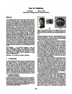
Figure 1: Comparison of our algorithm (per-band incremental or PBI) with standard (non-incremental) PRT. PBI integrates easily into existing frameworks, eg. image relighting (top) and clustered PCA (bottom). PBI (right) captures caustics(top) and sharp shadows (bottom) which at these framerates are blurred by non-incremental methods (left). Insets compare quality of the lighting approximation.
R. Overbeck, A. Ben-Artzi, R. Ramamoorthi, & E. Grinspun / Exploiting Temporal Coherence for Incremental All-Frequency Relighting
the difference in lighting between consecutive frames. Besides further accelerating PRT, our approach naturally yields a solution which quickly and smoothly converges to an exact (up to the approximation of the transport T ) representation of L under static or slowly varying lighting. Our specific contributions are: Analysis of Temporal Coherence: This paper explores temporal coherence as a key avenue for further research and compression in PRT methods. A series of experiments (see Sec. 4) on a rotating lighting environment exposes (i) the approximations and artifacts of alternative algorithms, and (ii) the inherent spatio-temporal coupling of the coherence in complex illumination (see Fig. 5). Per-Band Incremental (PBI) Wavelet Algorithm: We develop an algorithm (see Sec. 5) that adapts to the temporal coherence of each wavelet level, dynamically choosing an incremental update over standard NWA when profitable. The results, compared to standard PRT methods, are often dramatic (see Fig. 1), and free of the flickering and ghosting artifacts of a straightforward basic incremental (BI) method (Sec. 3). When the evolution of the lighting is slow, static or changes only over a sparse set of directions, PBI is able to incrementally update all the wavelet bands, preserving or approaching a nearly exact solution. Even when the lighting changes rapidly, PBI preserves temporal coherence of the coarser wavelets. Integration with PRT Methods: PBI integrates easily into existing all-frequency methods: it leaves open the alternatives for precomputing and representing T . We demonstrate PBI in the context of the original image relighting method [NRH03], the extension to changing view using BRDF factorization [WTL04], and clustered PCA [LSSS04] (see Sec. 6). In all cases, only about 100 lines of extra code is required, and time and memory overheads are negligible. While the lighting is changing dynamically, our method can usually lead to improvements by a factor of three or four. We obtain high-quality all-frequency effects with only 30 wavelet lighting terms per frame (see Fig. 1), comparable to the coefficient budget of low-frequency spherical harmonic methods. Within a few frames of the lighting remaining static (the user being idle), we converge to the exact result. The exact solution is maintained even under changing viewpoint in methods such as [LSSS04, WTL04]. 2. Previous Work Precomputation-based relighting or radiance transfer (PRT) was introduced by Sloan et al. [SKS02, SHHS03, SLS05], building on prior work on design of time-dependent lighting by Dorsey et al. [DAG95] and others. Much of this work focuses on low-frequency effects, using spherical harmonics [RH01]. We will discuss these methods briefly in Sec. 7 and in greater detail in [Ove06], but here we focus primarily on all-frequency relighting [NRH03], which reproduces a richer class of visual effects and stands to benefit more from leveraging temporal coherence. We work with the fundamental algorithms [NRH03, WTL04, LSSS04], that form the building blocks for allfrequency PRT. Our focus is on real-time rendering— thus, we do not consider all-frequency triple product algorithms [NRH04, ZHL∗ 05] that are not real-time. Recent advances (e.g., translucent materials [WTL05]) fit into our approach as they are variants of Eq. 1, differing only in the
transport matrix T . Since we change the representation of L only, our method can be easily integrated into most existing PRT algorithms. The ideas for the basic incremental (BI) algorithm (see Sec. 3) were also motivated by our concurrent work on manipulating 1D curves for editing BRDFs ( [Ano06] Sec. 6). In general, the literature in rendering, and even beyond graphics, is rich in its coverage of temporal coherence. Since most of these previous approaches are not suitable for PRT algorithms, we give only a brief survey. One may imagine applying video compression [SS00] to a pre-defined lighting sequence. However, the size of the lighting is small compared to the size of the transport matrix T . Moreover, the lighting sequence in an interactive system is not predetermined. Finally, our goal is really to accelerate the matrix-vector multiplication in Eq. 1, which is not sped up by compression techniques such as optical flow or sparse bitrate coding. For offline rendering of dynamically-lit animations, Wan et al. [WWL05] exploit temporal coherence in importance sampling environment maps to reduce flickering. They build adaptive spherical quad-trees for creating point-samples in a raytracing framework, whereas PRT necessitates a function (wavelet) basis in Eq. 1. While reduced flicker is a side benefit of our approach, our main focus is on improved efficiency for real-time rendering. In frameless rendering [BFMZ94, DWWL05], pixels update asynchronously, while in our approach, wavelet lighting coefficients update asynchronously; combining these orthogonal approaches remains future work. 3. Basic Incremental (BI): A Didactic Example Consider a basic incremental wavelet algorithm that leverages temporal coherence in L. This algorithm, which motivates the remainder of the paper, will need significant improvement later, so we call it basic incremental (BI). To be concrete, consider equation 1 and [NRH03] (NWA) as the initial, non-incremental framework . L is the lighting vector in a full wavelet basis. First, we rewrite Eq. 1 to make the approximation explicit, B = T L˜ ,
(2)
where L˜ = Approx(L) is the (compressed) lighting vector in a truncated wavelet basis (typical dimension 30–200). Our basic idea is to consider the change in lighting from the previous frame, ∆L, replacing Eq. 2 with the incremental update, Bnew = Bold + ∆B ∆B = T ∆L .
(3) (4)
The computational and memory overhead is minimal. Storage of the previous frame Bold is negligible compared to the size of T , and the cost of computing Eq. 3 is negligible relative to the matrix-vector multiplication in Eq. 4 (or 2). Our insight is that ∆L is much more compressible than L. Therefore we write, � ∆L = Approx Lnew − L˜ , (5) ˜L = L˜ + ∆L . (6) c The Eurographics Association 2006.
R. Overbeck, A. Ben-Artzi, R. Ramamoorthi, & E. Grinspun / Exploiting Temporal Coherence for Incremental All-Frequency Relighting
Frame =
1 : Initial
30 : Initial
75 : Intermediate
125 : Intermediate-Final
400 : Final
NonIncremental 30 Wavelets
Reference 24576 Wavelets
Exact
1b
a = Reference b = Basic Incremental c = PBI 1c 2a 2b 2c
Ghosting
1b
Ghosting and Artifacts 2b
1c
No Ghosts Drop High Frequencies 2c
Still Good
Per-Band Incremental 30 Wavelets
Frame 75 1a
2a
Still Good
Basic Incremental 30 Wavelets
Exact
1a
Frame 125 3a
Artifacts
3a
4a
Converged
3b
Converging Still Ghosts 4b
Converging
Converged
3c
4c
a = Reference b = Basic Incremental c = PBI 3c 4a 4b 4c
3b
Converging, Still Artifacts
Ghosting
Figure 2: Comparison of lighting approximations with 30 wavelet terms, for rotating the Grace Cathedral cubemap. The top row is NWA (non-incremental PRT), followed by the reference image, the basic incremental BI algorithm from Sec. 3, and the per-band incremental PBI method to be developed in Sec. 5. The bottom row shows details that reveal the performance and artifacts of the different algorithms. We use a tilde for L˜ in Eq. 6, to signify that it is a wavelet approximation to the lighting, which is updated at each frame. Basic Incremental (BI) algorithm: Eqs. 3, 4, 5 and 6 make up the most basic approach to an incremental lighting update. The method leverages the observation that Lnew − L˜ can be more aggressively and sparsely approximated than Lnew . To initialize , we usually set L˜ 0 = L0 at the intial frame 0 by computing the full matrix-vector multiply in Eq. 1. In our implementation, we adopted the Haar wavelet basis on a 6 × 64 × 64 cubemap [NRH03]. However, there is nothing in the above discussion that restricts the basis representation used. Besides the high compressibility of ∆L, a useful property of BI is that it progressively converges to the exact result when the user is idle (lighting Lnew is static) in a design session. Observe that a constant Lnew acts as a fixed point under repeated iteration of BI. In contrast, all current PRT algorithms will maintain a static approximate image using L˜ from Eq. 2. Moreover, when the lighting change is sparse (ie. moving and resizing an area light source) convergence is often achieved in a single timestep. c The Eurographics Association 2006.
Frame = 30
75
400
NonIncremental 30 Wavelets Blurred Shadows and Highlights
Reference 24576 Wavelets
Ghost Shadow
Exact
Basic Incremental 30 Wavelets
Figure 3: Rendered images for the lighting sequence in Fig. 2, comparing NWA (top), the reference (middle), and basic incremental BI (bottom). A comparison of BI with the PBI method is shown later, in Fig. 8.
R. Overbeck, A. Ben-Artzi, R. Ramamoorthi, & E. Grinspun / Exploiting Temporal Coherence for Incremental All-Frequency Relighting Coverage Color Key (overlapping colors add)
Single Frame Coverage Frame =
29
30
74
4096 1024 256 64
Wavelet Area
75
16
4
125
124
Basic Incremental 30 Wavelets
NonIncremetal 30 Wavelets
Basic Incremental NonIncremental
100 80 60 40 20
121
125
120
120
100
100 Number Chosen
NonIncremetal 30 Wavelets
120
Number Chosen
Basic Incremental 30 Wavelets
5 Frame Accumulated Coverage and Histograms 30 71 75
26
Number Chosen
Frame =
80 60 40 20
80 60 40 20 0
0
4096 1024 256 64 16 4 Wavelet Areas
0
4096 1024 256 64 16 4 Wavelet Areas
4096 1024 256 64 16 4 Wavelet Areas
Figure 4: Top: Coverage maps for incremental (BI) and non-incremental (NWA) algorithms for some frames from Fig. 2. Bottom: Histogram and averages, over a 5 frame interval, of which wavelets and wavelet levels are chosen by incremental (BI) and non-incremental (NWA) algorithms. 4. Analysis of Temporal Coherence We conducted experiments to better understand BI and more generally temporal coherence of dynamic lighting. The observations in this section motivate the robust, efficient PBI method in Sec. 5. 4.1. Comparison of Incremental and Non-Incremental Consider a rotation of the Grace Cathedral lighting environment. Figs. 2 and 3 depict temporal evolution of the lighting cubemap and the rendered image, respectively (see also Fig. 9–bottom). This example is representative of numerous experiments spanning a range of light manipulations, scenes, and shading complexities. Rotations are the most challenging test because the illumination is dynamic almost everywhere. We compare NWA, reference, BI, and (for completeness) PBI, always using 30 wavelet terms. Initial Frames: Initially (frame 0) L˜ 0 = L0 , and BI’s lighting approximation exactly matches the reference. Indeed, early on, while rotation is relatively slow, BI’s lighting approximation is significantly sharper and more accurate than NWA’s (see frame 30, Fig. 2). The resulting images (see Fig. 3) also display much sharper shadows, accurately matching the reference. Intermediate Behavior and Artifacts: Next, consider intermediate times (see frame 75 in Figs. 2 and 3). The lighting now differs significantly from its intial state, and rotation rate is relatively fast. BI’s quantitative error is still smaller than NWA’s. Even so, while BI’s shadows and lighting continue to be sharper than NWA’s, they are inaccurate and spurious in many locations. Fig. 2-(1a/1b) highlights undesirable ghosting artifacts. For instance, consider the small bright light in the inset.
With its limited wavelet budget, BI cannot keep up, with lights leaving trails or ghosts in the old locations. This can lead to spurious sharp shadows in the images (see frame 75, Fig. 3). There are also significant high-frequency artifacts (see insets 2a–2b, Fig. 2) where BI cannot approximate the lighting sharply enough. In Sec. 5, we introduce a per-band incremental algorithm (PBI) which avoids these artifacts by using an incremental update only for wavelet bands that have sufficient temporal coherence; compare Fig. 2-(1b/1c) or Fig. 2-(2b/2c). Final Frames and Convergence: We stop the rotation sequence at frame 99, and let the lighting be static. As discussed in Sec. 3, this allows the incremental algorithm to converge to the correct lighting. Since we are using 30 wavelets per timestep, frame 125 in Fig. 2 is effectively using a 750-term wavelet approximation, and some regions have begun to converge (compare insets 4a and 4b). However, the previous ghosting is severe enough that some regions still show artifacts (compare insets 3a and 3b). Moreover, note from the insets that the PBI method in Sec. 5 is essentially converged at frame 125. Finally, at frame 400, the incremental algorithm has converged fully, and the image in Fig. 3 accurately matches the reference. 4.2. Detailed Analysis of Temporal Coherence We now show some more detailed results, characterizing the nature of temporal coherence. Coverage of Wavelets in Incremental and NonIncremental: In Fig. 4, we compare which wavelets are updated at each frame (what the coverage of the lighting is) for non-incremental NWA, versus incremental BI. Similar results also hold for the PBI method. From the top of Fig. 4, we see that BI by design upc The Eurographics Association 2006.
Temporal TEM P OR ALFRWavelet EQU NC Y Size
R. Overbeck, A. Ben-Artzi, R. Ramamoorthi, & E. Grinspun / Exploiting Temporal Coherence for Incremental All-Frequency Relighting
Per-Band Incremental Wavelets (PBI)
2 4
Procedure SetupBands() // Described in Sec. 5.2 for all Bands i IsIncri = Incremental(i); // Should band i be incremental Wi = Wavelets(i) ; // Which wavelets in i to update end ; Procedure PBI() // Per-Band Algorithm 5. SetupBands() ; 6. for all Bands i 7. if IsIncri // Update incrementally 8. for all chosen wavelets j in W i ˜ 9. ∆L j = Lnew // Eq. (5) j −Lj ; new ˜ 10. Lj = Lj ; // Eq. (6) 11. Bi = Bi + T j ∆L j ; // Eqs. (3) and (4) 12. end; 13. else // Update non-incrementally 14. Bi = 0 ; L˜ Band i = 0 ; // Zero or reset lights and image 15. for all chosen wavelets j in W i 16. L˜ j = Lnew ; // Eq. (6) j 17. Bi = Bi + T j L˜ j ; // Eq. (2) 18. end; 19. end ; 20. B = ∑6i=1 Bi ; // Sum over all bands 1. 2. 3. 4.
8
16
32 64
128 4096
1024
S P A
256 TIA LF
64
RE Q U E N C
Y
16
4
Spatial Wavelet Area Figure 5: A study of temporal coherence, independent of any algorithm. We show the norm of energy (darker is more) in each spatio-temporal wavelet band, as measured for the (uncompressed reference) rotation sequence of Fig. 2. Columns correspond to spatial bands, rows to temporal bands, and the evident diagonal structure implies that progressively finer spatial bands exhibit progressively diminishing temporal coherence. dates different regions of the environment at adjacent frames (once a wavelet is updated, the change in the next frame will not usually warrant it being updated immediately again). By contrast, essentially the same wavelets are chosen at adjacent frames for NWA. In these images, a pixel is shaded based on how many of the wavelet levels that overlap it are chosen at each frame. Coarser blocks indicate coarser wavelet coverage, and finer blocks indicate finer coverage in those regions. The bottom of Fig. 4 considers the cumulative result over 5 frames of lighting motion. NWA has a cumulative coverage that looks very similar to each individual frame. By contrast, BI updates a large number of wavelets with much finer frequencies. The bottom of Fig. 4 also shows a histogram of how many wavelets are updated at each level. NWA must always choose low-frequency coarse wavelets, that usually have the greatest energy. In fact, levels finer than 256 are not chosen at all, so the effective resolution of the environment map is only 6 × 8 × 8. However, we will see that these coarse wavelets also exhibit the greatest temporal coherence, and BI only needs to update them once every several frames to maintain an accurate approximation. Hence, many more terms can be devoted to finer wavelets, producing a more uniform distribution into finer levels, and higher-quality images that use an effectively higher resolution environment map. It is also instructive to compare the three frames (columns) in Fig. 4. On the left (frame 30), BI can keep track of very high frequencies, as seen in the histogram. In the middle (frame 75), the lighting rotation is faster, and more updates must be given to lower frequencies, somewhat reducing the effective resolution. Towards the end (frame 125), the lighting is static and the approximation is converging, with work focused exclusively on the higher-frequency or smaller wavelet bands. By contrast, non-incremental NWA always updates essentially the same (coarse) wavelet levels. Relation of Spatial Frequency and Temporal Coherence: Fig. 5 visualizes temporal coherence, independent of any specific practical algorithm. We take the first 128 frames of the rotation sequence, wavelet transformed along the spatial (angular) dimensions in the normal way, and then apply a c The Eurographics Association 2006.
Figure 6: Pseudocode for Per-Band Incremental Wavelet Algorithm (PBI). 1D Haar transform along the time dimension. We plot the total energy for given spatial and temporal wavelet bands, with darker regions having more energy. The coarsest spatial wavelets with area 4096 = 64 × 64 have almost all of their temporal energy in the lowest frequency temporal band (size 128). As we go to finer spatial wavelets, there is more energy in finer temporal wavelets—the visible diagonal structure indicates that the extent of temporal coherence decreases with spatial wavelet frequency. Unfortunately, the basic incremental algorithm treats each band similarly, which (due to the dark upper-right quarter of Fig. 5) can lead to ghosting and artifacts at high spatial frequencies. 5. Per-Band Incremental Wavelet Algorithm Building on these observations, we propose a per-band incremental (PBI) lighting update algorithm that treats each wavelet band separately, choosing either an incremental or non-incremental approach, based on the available temporal coherence. 5.1. Basic Per-Band Algorithm First, we group wavelets having area 4096 = 64 × 64 (the coarsest wavelet and scaling function) into one band, those with area 1024 = 32 × 32 (the next coarsest) into another band and so on. Since we consider cubemaps with resolution 64 × 64, there will in general be 6 wavelet levels or bands. For each band separately, we will decide whether to update it incrementally, as per Sec. 3, or in the standard nonincremental fashion, as per Eq. 2. The details of our algorithm are summarized in Fig. 6. First, we set up all the bands, determining whether they are updated incrementally or not (lines 2 and 5). How we do this optimally is a critical part of our algorithm, discussed in Sec. 5.2. Then, we must choose which wavelets to update (line 3). This is straightforward, since we simply need
R. Overbeck, A. Ben-Artzi, R. Ramamoorthi, & E. Grinspun / Exploiting Temporal Coherence for Incremental All-Frequency Relighting
Percentage Area-Weighted L1 Error
30
25
Per-Band Incremental 30 Wavelets 16 Simple 15 Exhaustive
20
13
NWA 30 Wavelets
14
BI 30 Wavelets
12 55 NWA 60 Wavelets
15
Basic Incremental (BI) (30 Wavelets) Ghosts and Artifacts
85
NWA 100 Wavelets
10
5 0
70
Frame 75 : Intermediate Per-Band Incremental (PBI) (30 Wavelets) No Ghosts or Artifacts Higher Frequencies Removed
PBI Simple 30 Wavelets
NWA 500 Wavelets
0
50
100 Frame
150
200
Figure 7: Comparison of lighting accuracy over time for different algorithms (standard or non-incremental NWA, incremental BI, per-band incremental PBI). The inset compares the two selection methods for PBI. to sort them in the standard way based on their magnitudes. We use area weighting for choosing wavelets, as recommended in [NRH03]. If a band is updated non-incrementally, we use the area-weighted magnitude of wavelet j, Area( j) | Lnew | for sorting; otherwise, we use the difference Area( j) | j ˜ ∆L j |= Area( j) | Lnew j − L j |. We treat each band separately (line 6), eventually summing their contributions (line 20). If the band is updated incrementally (lines 8-11), we use Eqs. 3–6. For each wavelet j in that band’s approximation, we compute the change ∆L j relative to the current value L˜ j (line 9), and also bring the current value up to date (line 10). In line 11, we add the contributions to the band image Bi . Since we are considering a single wavelet j, we will use a single column T j of the transport matrix. If the band does not have sufficient temporal coherence for an incremental update, it is simply updated as in standard PRT (line 17). We still update L˜ j = Lnew in line j 16, because future frames can (and usually will) still choose to update the band incrementally. 5.2. Selecting When to Update Incrementally We need to know when there is enough temporal coherence to update a band incrementally. One possibility is to let the user specify a threshold, with coarser bands updating incrementally, and finer bands using standard PRT. However, a static threshold is difficult to specify or adapt to different speeds of motion. Ideally, we would like the algorithm to automatically pick coarser bands for incremental updates when the lighting changes rapidly, and finer bands for slower lighting changes where there is more temporal coherence. We have tested several automated approaches that range from exhaustive and expensive, to very simple and efficient. We describe two of them below. 5.2.1. Exhaustive Search We consider every possibility for incremental vs nonincremental update over all bands, and pick the one that results in the least error for the lighting. For N wavelet bands, there are 2N possibilities. While this method imposes too much computational overhead to be practical, it is exhaustive (optimal within the scope of one frame) and therefore serves as a useful baseline to compare alternatives.
Figure 8: Comparison of images from PBI and basic incremental BI. 5.2.2. Simple and Fast Per-Band Test At the other extreme, we simply test each band separately, determining whether it is better approximated incrementally or not. To do so, we compare the norm for each band k Lnew − L˜ k with k Lnew k. If the former has a smaller error, we use an incremental update, using non-incremental otherwise. In practice, we find the L1 norm best for the quality of the final images, although similar quantitative results are also obtained with L2 . Note that non-incremental updating can be thought of as incremental with a previous value of 0, and our comparison is equivalent to seeing if the new light˜ This ing is closer to 0 or to the current approximation L. makes it explicit that the lighting can sometimes drift so far from the current approximation, that it is better to reset or zero the band. The method is greedy because the error comparison is done once at the beginning, before knowing how many wavelet terms are actually allocated to the band. Because of its simplicity, this algorithm has little computational overhead, and is very easy to implement. 5.3. Results and Discussion We now discuss some properties of the PBI algorithm and compare it with basic incremental BI and non-incremental NWA methods. Fig. 7 plots the area-weighted L1 error for the sequence in Fig. 2. PBI clearly out-performs BI and non-incremental NWA. Moreover, it converges faster than BI. Note that BI always performs better quantitatively than NWA, but has relatively large errors in the middle of the rotation sequence because of the ghosting and artifacts. Its performance is close to PBI in the early part of the sequence, when both methods accurately approximate the lighting. The inset in Fig. 7 compares the two methods just discussed for selecting whether or not to update incrementally in PBI. In most cases, both approaches perform nearly identically—we do not show both curves in the main plot since one cannot distinguish them at that scale (the error axis in the inset is magnified). There are only marginal improvements for exhaustive over the simple per-band test. Hence, because of its implementation simplicity and low computational overhead, we will always use the simple test. We can also attempt to see how many wavelets are needed in standard PRT to produce equal quality results as PBI. Because of the fundamentally different nature of the algorithms, we plot a number of curves in Fig. 7. PBI with 30 wavelets is essentially always better than standard nonc The Eurographics Association 2006.
R. Overbeck, A. Ben-Artzi, R. Ramamoorthi, & E. Grinspun / Exploiting Temporal Coherence for Incremental All-Frequency Relighting Time
averaged 14.2 frames per second, and standard NWA averaged 14.8 fps. Since the computational overhead for PBI is minimal, we refer to the number of wavelets used to quantify performance through out this paper (rather than running times that are implementation and machine-specific).
4096 Wavelet Area
1024 256 64 16
6. Integration with PRT methods
Rotation Angle (degrees)
4 40
Rotation Starts
In this section, we integrate our per-band incremental (PBI) wavelet algorithm into the methods that form the basic building blocks for all all-frequency PRT algorithms, showing a variety of results.
Rotation Ends
30 20 10 0
6.1. Basic Image Relighting 11
30
75 99 Time (Frames)
125
Figure 9: Incremental (horizontal line) vs non-incremental (vertical line) updates for different bands using PBI. Bands are occasionally reset, or evaluated non-incrementally, when they drift too far from the stored value, with more frequent resets for higher frequency or finer wavelets. incremental NWA with 60 wavelets. Moreover, approximately 100 wavelets in non-incremental are needed to be comparable (sometimes better, sometimes worse) to PBI over the full sequence, while the lighting is rotating. However, if we include the static regions, where PBI converges, even a 500 wavelet non-incremental approximation cannot achieve equal quality as our method within 25 time steps of stopping rotation. Fig. 8 compares PBI to BI (for intermediate frame 75 from Fig. 3). We can clearly see a sharp shadow without the ghosting and artifacts. Similarly, Figs. 1 and 2, and the closeups, clearly show that PBI significantly outperforms BI and standard PRT. Fig. 9 shows the characteristic behavior of PBI for different wavelet sizes or bands. The vertical lines correspond to frames where that band was updated non-incrementally. As can be seen, the bands update incrementally most of the time, but are occasionally reset or zeroed out, updating nonincrementally for that frame. The frequency of restarting (non-incremental frames) depends on the speed of motion (lighting change) and wavelet level. Coarser wavelets exhibit greater temporal coherence—in fact, the two coarsest levels (sizes 4096 and 1024) always update incrementally. As the wavelet level gets finer, restarting becomes more frequent. PBI automatically adapts the frequency of restarts, or nonincremental updates, to the rate of illumination change and wavelet level. Finally, we consider the computational and memory overhead for PBI. The memory overhead is primarily the stored value or previous frame’s (floating point 512 × 512) image for each of the 6 wavelet bands. Together with (small) auxiliary data structures, the total extra storage is 19.2 megabytes. By comparison, the transport matrix and auxiliary structures for the scene in Fig. 2 occupy 229 MB, and this can be larger for more complex scenes. Hence, the memory overhead is only 8% for this scene. The computational overhead comes primarily from adding the per-band images in line 20 of Fig. 6. This is a fixed cost, and the relative time decreases as we increase the wavelet budget. Even if we only update 1 wavelet per frame, the overhead is only 20%. For realistic wavelet budgets, such as the dynamic lighting sequence in Fig. 2 with 30 wavelets, the overhead is less than 5%—PBI c The Eurographics Association 2006.
We have already seen basic image relighting [NRH03] in Figs. 1 (top), 2 and 8. For implementation, we simply modified the code framework in [NRH03] to incorporate PBI. The modifications affected only the lighting approximation and matrix multiplication phases, and required only about 100 lines of additional code. Figure 10 shows another example on a 512 × 512 image of the plant scene with intricate shadowing. We compare closeups as we increase the number of terms in both PBI and standard PRT. For equal time (30 or 100 wavelets), PBI has significantly sharper shadows in dynamic lighting. Three to four times as many terms are needed in standard PRT for equal quality across a fair range of wavelet approximations (about 100 in standard for 30 wavelets in PBI, and 300 in standard for 100 in PBI). Finally, within 5 frames of stopping lighting motion, PBI has essentially converged, and a 30 term approximation is comparable to 300 terms in standard PRT. Since the quality of the image (such as the sharpness of shadows) in PBI depends on the speed of lighting variation, the shadows will get softer or sharper as the user speeds up or slows down the change in lighting. In many applications, such as lighting design, this is a very desirable behavior, with low-frequency feedback for rough lighting placement and all-frequency for fine adjustments. In some other applications, this change in quality may sometimes be interpreted as undesirable flickering—however, all non-linear wavelet approximation methods exhibit some flicker. This flicker can be reduced by increasing the wavelet budget. For example, 100 PBI wavelets (equivalent to 300 NWA wavelets during rotation) is essentially artifact free. 6.2. Changing View with BRDF Factorization We now consider the extension to varying view as well as lighting, taking glossy materials into account using the methods of [LSSS04, WTL04]. Those methods use an in-out factorization of the BRDF, with a separate Tk for each BRDF term k. To take advantage of temporal coherence, we simply apply PBI to the lighting once, and then use this lighting approximation for all k, and each matrix-vector multiplication Tk L. Again the PBI method can be integrated in less than a hundred lines of code. It involves negligible computational or memory overhead and results in the same 3×–4× improvement and converges as before. 6.3. Clustered PCA Clustered PCA [LSSS04, SHHS03] or CPCA compresses the transport matrices T using spatial coherence, for greater
R. Overbeck, A. Ben-Artzi, R. Ramamoorthi, & E. Grinspun / Exploiting Temporal Coherence for Incremental All-Frequency Relighting PBI (30 Wavelets)
NWA (30 Wavelets)
30 Wavelets
100 Wavelets
300 Wavelets
PBI
PBI
PBI
NWA
NWA
NWA
Frame 45 (While rotating)
Frame 117 (5 frames after stopping)
PBI
PBI
PBI
NWA
NWA
NWA
Figure 10: Comparison of different numbers of wavelet terms for PBI and standard NWA, while rotating (top) and within 5 frames of stopping (bottom). On top, we see that three to four times as many wavelet terms are needed for equal quality in standard PRT. Moreover, about 10 times as many terms is needed within a few frames of stopping (bottom). For equal time, with the same number of wavelets, PBI consistently has much sharper shadows than standard PRT. compactness and efficiency. The vertices of the scene are broken into clusters, each of which is approximated with a low-dimensional PCA basis. We emphasize that our method can be applied “blindly” with any representation of T , including CPCA, since we simply modify the lighting approximation L. However, even greater speedups can be obtained if we understand the CPCA method, and modify it to be fully incremental, as described below. In the first rendering step, CPCA computes per-cluster coefficients, Pic = Mic L,
(7)
where the superscript denotes the cluster number c, and the subscript denotes the PCA basis function i. Mic can be thought of as a K × N matrix, where N is the lighting resolution (in our case 6 × 32 × 32). For glossy objects( [LSSS04], [WTL04]), each row of Mic corresponds to a specific term k in the BRDF factorization, and each element of the K element vector Pic is a dot product of this row in Mic and the lighting vector L. In the second rendering step, the per-vertex weights are used to blend the coefficients Pic , with Uv =
S
∑ wvi Pi
c(v)
,
(8)
i=1
where v is the vertex, c(v) is its corresponding cluster, wvi is the weight for vertex v and basis function i, and we sum over all S PCA basis functions i. Note that U v is a K element vector, with a separate value for each term of the BRDF. The final step weights by the BRDF factors gk , Bv (ωo ) =
K
∑ gk (ωo )Ukv .
(9)
k=1
Step 3, (Eq. 9) is usually very efficient, since K is small, and we compute it in the standard way. In [LSSS04], step 2, (Eq. 8) is expensive, since it is done for each vertex— but is usually much more efficient than standard PRT, since one needs to sum over only S basis functions. Getting very
sharp all-frequency shadows requires a large number of clusters, as well as more PCA basis functions than used by a low-frequency implementation ( [SHHS03]). In this regime, steps 1 and 2 have comparable computational expense (as they do in the related technique of [NBB04]), and we would ideally like both steps to exploit temporal coherence. Step 1 (Eq. 7) has essentially the same form as Eqs. 1 and 2, and we can directly apply the PBI method to L. Step 2 (Eq. 8) is more interesting. For a given BRDF term k and cluster c, we can concatenate the weights wvi for all i into a large matrix W , whose rows correspond to vertices and columns to coefficients i. In that case, step 2 becomes U = W P,
(10)
where P is an S-element vector of (dynamically-changing) coefficients for that cluster. We now have a very similar form to Eq. 1, with the vector P taking the place of the lighting. Since there is no clear concept of bands, we apply the basic incremental algorithm of Sec. 3, which works well since S is usually small. We usually choose the number of incremental terms to be S/4, which gives us a four-fold improvement, while maintaining a high accuracy solution that avoids ghosting. In summary, we perform both steps of CPCA rendering incrementally, with PBI wavelets used for step 1 (lighting approximation and per-cluster coefficients), and basic incremental used for step 2 (per-vertex weights). Figs. 11 and 12 show a complex scene, with 40,029 vertices (largely on the ground plane to capture intricate shadows), 398 clusters, S = 25 PCA bases, and complex BRDFs (note the fairly sharp Phong highlights on the street lamps, especially in the right column of Fig. 11—we use K = 4 BRDF terms) . We use 6 incremental basis functions per cluster in Fig. 11. We render this complex scene at real-time rates. Another example is shown in the bottom of Fig. 1. In both cases, our algorithm captures significantly sharper shadows than standard CPCA. To stress the generality of our method, the first two columns of Fig. 11 show two types of light manipulation— rotation as before, and interpolating two environments (Grace and StPeters). Note that the view can also simultanec The Eurographics Association 2006.
R. Overbeck, A. Ben-Artzi, R. Ramamoorthi, & E. Grinspun / Exploiting Temporal Coherence for Incremental All-Frequency Relighting
Rotating the Lighting Environment
Interpolating the Lighting Environment
Changing View (Constant Lighting)
NonIncremental (NWA) 30 Wavelets
PBI Simple 30 Wavelets
Non-Incremental (NWA) 100 Wavelets
Figure 11: Comparison of images with standard PRT and PBI for 30 wavelets, as well as standard PRT with 100 wavelets (which is marginally worse quality than the 30 term PBI approximation). For dynamic lighting (first two columns), PBI produces much sharper shadows than PRT with the same number of wavelet terms. We obtain exact results when only the view is changing in the right column—in this case, PBI is much sharper than the 100 term non-incremental result. PBI + Incremental PCA Bases 100 Wavelets, 6 PCA Bases
Non-Incremental (NWA) 100 Wavelets, 6 PCA Base
CPCA Clusters
2 PCA Bases
4 PCA Bases
6 PCA Bases
25 PCA Bases Non-Incremental Wavelets (300) + Incremental Bases Non-Incremental Wavelets (300) + Non-Incremental Bases
Figure 12: CPCA, using our temporal coherence algorithm. On left, we show the CPCA clusters color coded—we use several to accurately capture sharp shadows. On right, we compare our method with standard CPCA, clearly showing the higher quality in the images. The closeups below show the effect of changing the number of incremental terms in the second step of CPCA, and we see that S/4 = 6 is enough for very high quality (in the closeups, we always use high quality non-incremental updates for the lighting projection (first) step, so we can focus only on comparing incremental and non-incremental PCA bases).
c The Eurographics Association 2006.
R. Overbeck, A. Ben-Artzi, R. Ramamoorthi, & E. Grinspun / Exploiting Temporal Coherence for Incremental All-Frequency Relighting
ously change in these examples. As seen in the bottom row, even 100 wavelet terms in standard PRT performs somewhat worse than PBI. In the third column, we change viewpoint only. Since the lighting is static, the PBI algorithm very rapidly converges to the exact solution, which is accurately maintained while changing view, and is much sharper than the 100 term standard PRT comparison. The closeups in the bottom row of Fig. 12 show how the quality improves as we increase the number of incremental terms in step 2 (Eq. 10). Clearly, S/4 = 6 terms suffices to give almost reference quality images in dynamic lighting. Hence, as with the earlier algorithms, we get a performance improvement by a factor of about four for both steps of CPCA in dynamic lighting, with rapid convergence in static lighting even if the view changes. 7. Conclusions and Future Work We have explored a critical source of coherence and compression in all-frequency PRT methods—temporal coherence in the lighting. We have analyzed the nature of temporal coherence, and developed an efficient per-band incremental wavelet algorithm. The method is very simple to implement and can be integrated with essentially all current real-time all-frequency PRT methods, while imposing minimal computational or memory overhead. For dynamicallyvarying lighting, we can obtain a performance improvement of 3×–4× without sacrificing quality. Equivalently, we can substantially increase the quality of all-frequency PRT methods, without sacrificing speed. Moreover, our algorithm converges to the exact result within a few frames of the lighting being static. There is nothing in Eqs. 1 and 2 restricting us to use wavelets or all-frequency methods. Indeed, we have conducted some preliminary experiments with spherical harmonics [Ove06]. With a slightly modified PBI algorithm, we were able to achieve comparable improvements as for wavelets, although the visual benefits are less dramatic. [NRH03] concluded that NWA converges exponentially faster than a linear harmonic approximation as the number of terms increases. Therefore, PBI for spherical harmonics converges exponentially slower than for wavelets. More research is needed to determine the best way to integrate the incremental method into low-frequency approaches, and efficient GPU implementations of those methods. Finally, we have exploited temporal coherence only in the lighting for static scenes. One could also exploit temporal coherence of the transport matrices for dynamic scenes, in applications like lighting design for pre-determined animated sequences. We predict that future PRT and other highquality real-time rendering algorithms will be designed to take full advantage of temporal coherence in lighting, viewpoint and scene geometry. 8. Acknowledgements This research was funded in part by a Sloan Research Fellowship and NSF grants #0305322 and #0446916. We thank Ren Ng for making available his code frameworks and scenes for all-frequency relighting.
References [Ano06] A NONYMIZED: Real-time BRDF editing in complex lighting. In Accepted to SIGGRAPH 06 (2006).
[BFMZ94] B ISHOP G., F UCHS H., M C M ILLAN L., Z A GIER E.: Frameless rendering: Double buffering considered harmful. In Proceedings of SIGGRAPH (1994), pp. 175–176. [DAG95] D ORSEY J., A RVO J., G REENBERG D.: Interactive design of complex time dependent lighting. IEEE Comp. Graph. and Apps. 15, 2 (March 1995), 26–36. [DWWL05] DAYAL A., W OOLLEY C., WATSON B., L UEBKE D.: Adaptive frameless rendering. In EGSR (2005), pp. 265–275. [LSSS04] L IU X., S LOAN P., S HUM H., S NYDER J.: Allfrequency precomputed radiance transfer for glossy objects. In EGSR (2004), pp. 337–344. [NBB04] NAYAR S., B ELHUMEUR P., B OULT T.: Lighting-sensitive displays. ACM TOG 23, 4 (2004), 963– 979. [NRH03] N G R., R AMAMOORTHI R., H ANRAHAN P.: All-frequency shadows using non-linear wavelet lighting approximation. ACM TOG (SIGGRAPH 03) 22, 3 (2003), 376–381. [NRH04] N G R., R AMAMOORTHI R., H ANRAHAN P.: Triple product wavelet integrals for all-frequency relighting. ACM TOG (SIGGRAPH 04) 23, 3 (2004), 475–485. [Ove06] OVERBECK R.: Exploiting Temporal Coherence for Pre-computation Based Rendering. Master’s thesis, Columbia University, 2006. CUCS-025-06. [RH01] R AMAMOORTHI R., H ANRAHAN P.: An efficient representation for irradiance environment maps. In Proceedings of SIGGRAPH (2001), pp. 497–500. [SHHS03] S LOAN P., H ALL J., H ART J., S NYDER J.: Clustered principal components for precomputed radiance transfer. ACM TOG (SIGGRAPH 03) 22, 3 (2003), 382– 391. [SKS02] S LOAN P., K AUTZ J., S NYDER J.: Precomputed radiance transfer for real-time rendering in dynamic, lowfrequency lighting environments. ACM TOG (SIGGRAPH 02) 21, 3 (2002), 527–536. [SLS05] S LOAN P., L UNA B., S NYDER J.: Local, deformable precomputed radiance transfer. ACM TOG (SIGGRAPH 05) 24, 3 (2005), 1216–1224. [SS00] S HI Y., S UN H.: Image and Video Compression for Multimedia Engineering: Fundamentals, Algorithms, and Standards. CRC Press, 2000. [WTL04] WANG R., T RAN J., L UEBKE D.: Allfrequency relighting of non-diffuse objects using separable BRDF approximation. In EGSR (2004), pp. 345–354. [WTL05] WANG R., T RAN J., L UEBKE D.: Allfrequency interactive relighting of translucent objects with single and multiple scattering. ACM TOG (SIGGRAPH 05) 24, 3 (2005), 1202–1207. [WWL05] WAN L., W ONG T., L EUNG C.: Spherical Q2tree for sampling dynamic environment sequences. In EGSR (2005), pp. 21–30. [ZHL∗ 05] Z HOU K., H U Y., L IN S., G UO B., S HUM H.: Precomputed shadow fields for dynamic scenes. ACM TOG (SIGGRAPH 05) 25, 3 (2005).
c The Eurographics Association 2006.