Exploiting Hierarchical Domain Structure to ... - Semantic Scholar

Exploiting Hierarchical Domain Structure to Compute Similarity PRASANNA GANESAN, HECTOR GARCIA-MOLINA, and JENNIFER WIDOM Stanford University

The notion of similarity between objects finds use in many contexts, for example, in search engines, collaborative filtering, and clustering. Objects being compared often are modeled as sets, with their similarity traditionally determined based on set intersection. Intersection-based measures do not accurately capture similarity in certain domains, such as when the data is sparse or when there are known relationships between items within sets. We propose new measures that exploit a hierarchical domain structure in order to produce more intuitive similarity scores. We extend our similarity measures to provide appropriate results in the presence of multisets (also handled unsatisfactorily by traditional measures), for example, to correctly compute the similarity between customers who buy several instances of the same product (say milk), or who buy several products in the same category (say dairy products). We also provide an experimental comparison of our measures against traditional similarity measures, and report on a user study that evaluated how well our measures match human intuition. Categories and Subject Descriptors: H.3.1 [Information Storage and Retrieval]: Content Analysis and Indexing General Terms: Algorithms Additional Key Words and Phrases: Similarity measures, hierarchy, collaborative filtering, data mining

1. INTRODUCTION The notion of similarity is used in many contexts to identify objects having common “characteristics.” For instance, a search engine finds documents that are similar to a query or to other documents. A clustering algorithm groups together gene sequences that have similar features. A collaborative filtering system looks for people sharing common interests [Goldberg et al. 1992]. In many cases, the objects being compared are treated as sets or bags of elements drawn from a flat domain. Thus a document is a bag of words, a customer is a bag of purchases, and so on. The similarity between two objects is often determined by their bag intersection: the more elements two customers This material is based upon work supported by the National Science Foundation under Grants IIS0085896, IIS-9817799, and IIS-9811947. Prasanna Ganesan is supported by a Stanford Graduate Fellowship. Authors’ address: 353 Serra Mall, #432, Stanford University, Stanford, CA 94305-9025; email: [email protected]. Permission to make digital/hard copy of all or part of this material is granted without fee for personal or classroom use provided that the copies are not made or distributed for profit or commercial advantage, the ACM copyright/server notice, the title of the publication, and its date appear, and notice is given that copying is by permission of the ACM, Inc. To copy otherwise, to republish, to post on servers, or to redistribute to lists requires prior specific permission and/or a fee. ° C 2003 ACM 1046-8188/03/0100-0064 $5.00 ACM Transactions on Information Systems, Vol. 21, No. 1, January 2003, Pages 64–93.

Exploiting Hierarchical Domain Structure

•

65

Fig. 1. Music CD hierarchy.

purchase in common, the more similar they are considered. In other cases, the objects are treated as vectors in an n-dimensional space, where n is the cardinality of the element domain. The cosine of the angle between two objects is then used as a measure of their similarity [McGill 1983]. We propose enhancing these object models by adding a hierarchy describing the relationships among domain elements. The “semantic knowledge” in the hierarchy helps us identify objects sharing common characteristics, leading to improved measures of similarity. To illustrate, let us look at a small three-level hierarchy on the music CD domain, as shown in Figure 1. Say customer A buys Beatles CDs b1 and b2 , B buys Beatles CDs b3 and b4 , and C buys Stones CDs s1 and s2 . If we were to use a similarity measure based on set intersections, we would find that the similarity between any two of A, B, and C is zero. The Vector-Space Model would represent A, B, and C as three mutually perpendicular vectors and, therefore, the cosine similarity between any two of them is again zero. However, looking at the hierarchy of Figure 1, we see that A and B are rather similar since both of them like the Beatles, whereas A and C are somewhat less similar since, although both listen to rock music, they prefer different bands. The similarity between two CDs is reflected in how far apart they are in the hierarchy. In this article, we develop measures that take this hierarchy into account, leading to similarity scores that are closer to human intuition than previous measures. There are several interesting challenges that arise in using a hierarchy for similarity computations. In our CD example, for instance, customers may purchase CDs from different portions of the hierarchy: for example, customer D in Figure 1 purchases both Beatles as well as Mozart CDs. In such a case it is not as obvious how similar D is to A or B or to other customers with mixed purchases. As we show, there are multiple ways in which the hierarchy can be used for similarity computations, and in this article we contrast different approaches. Another challenge is handling multiple occurrences (multisets) at different levels of the hierarchy. For example, say we had another user E who buys a lot of Beatles CDs as well as a Mozart CD m1 (see Figure 1). The question is: Which of D or E is more similar to A? Customer D bought Beatles CD b1 , just like A. On the other hand, customer E did not buy that CD, but did buy a lot of other Beatles CDs. The traditional cosine-similarity measure favors multiple occurrences of an element. That is, if a query word occurs a hundred times ACM Transactions on Information Systems, Vol. 21, No. 1, January 2003.

66

•

P. Ganesan et al.

in a document, the document is more similar to the query than one in which the query word appears only once. If we use this approach in our example, we would say that E is more similar to A than D is, because E buys 14 Beatles CDs, whereas D buys just one. Unfortunately, it is not clear that this conclusion is the correct one. E is probably a serious Beatles fan, whereas A and D appear more balanced and similar to each other, so it would also be reasonable to conclude that D is more similar to A than E is. Thus measures like cosine-similarity, although suitable for query-document similarity, do not provide the right semantics for interobject similarity in many other situations. This problem has, in fact, been observed earlier even in the context of inter-document similarity [Shivakumar and Garcia-Molina 1995]. In this article, we study various semantics for multiple occurrences, and provide measures that map to these semantics. There has been a lot of prior work related to similarity in various domains and, naturally, we rely on some of it for our own work. In Sections 2 and 6 we discuss prior work in detail, but here we make some brief observations. In our example we have seen that with traditional measures customers A, B, and C have zero similarity to each other because their purchases do not intersect. When objects or collections are sparse (i.e., have few elements relative to the domain), intersections tend to be empty and traditional measures have difficulty identifying similar objects. There have been many attempts to overcome this sparsity problem through techniques such as dimension reduction [Sarwar et al. 2000], filtering agents [Sarwar et al. 1998], item-based filtering [Sarwar et al. 2001], and the use of personal agents [Good et al. 1999]. We believe that using a richer data model (i.e., our hierarchy) addresses this problem in a simple and effective way. Hierarchies are often used to encode knowledge, and have been used in a variety of ways for text classification, for mining association rules, for interactive information retrieval, and various other tasks where similarity plays a role [Feldman and Dagan 1995; Han and Fu 1995; Scott and Matwin 1998; Srikant and Agrawal 1995]. In this article, we focus on the case where attributes are confined to being leaves of the hierarchy. We believe that our work may be extended to deal with polyhierarchies, where the hierarchy is not required to be a strict tree, to permit attributes at multiple levels in the hierarchy, and to deal with generalizations of hierarchies, where similarity relationships between attributes are used to induce similarity relationships between objects consisting of sets of these attributes. We do not cover these extensions in this article. Our goal here is to rigorously study how a domain hierarchy can be used to compute similarity between sets of leaves and to explore, compare, and evaluate the various options available. Different applications require different notions of similarity and we expect that an analysis of the specific application would determine which of our proposed similarity measures suits it the best. There are many domains in which hierarchies exist and can be exploited as we suggest here. For example, there is an inherent hierarchical structure to the URLs of pages within a single site. This structure can be exploited in clustering user sessions identified from a Web log [Joshi and Krishnapuram 2000; ACM Transactions on Information Systems, Vol. 21, No. 1, January 2003.

Exploiting Hierarchical Domain Structure

•

67

Fig. 2. Evolution of similarity measures.

Nasraoui et al. 1999]. Although Nasraoui et al. [1999] do attempt to exploit this hierarchical structure in computing similarity, the proposed similarity measure turns out to be highly unintuitive and can provide arbitrarily low values of similarity even between identical sessions. We would expect the use of our similarity measures to provide a dramatic improvement in the quality of the results. To name a few other examples, the Open Directory [OPD ] is a hierarchy on a subset of pages on the Web. Thus, we can compute the similarity of Web users, for instance, based on a trace of the Web pages they visit. In the music domain, songs can be organized into a hierarchy by genre, band, album, and so on. This hierarchy can then be used, say, to find users with similar tastes, and recommend new songs to them. In the document domain, we can use existing hierarchies such as WordNet [Miller et al. 1990] to compute document similarity. In all of these cases, our general-purpose extended similarity measures can be used to improve functionality. In summary, the main contributions of this article are the following. —We introduce similarity measures that can exploit hierarchical domain structure, leading to similarity scores that are more intuitive than the ones generated by traditional similarity measures. —We extend these measures to deal with multiple occurrences of elements (and of ancestors in the hierarchy), such as those exhibited in A and E in Figure 1, in a semantically meaningful fashion. —We analyze the differences between our various measures, compare them empirically, and show that all of them are very different from measures that don’t exploit the domain hierarchy. —We report the findings of a user study to evaluate the quality of the various measures. Figure 2 shows the evolution of the measures that we discuss, and serves as a roadmap for the rest of the article. Section 2 describes traditional measures of similarity. Section 3 introduces our First-Generation measures, which exploit a hierarchical domain structure and are obtained as natural generalizations of the traditional measures. Section 4 introduces the multiple-occurrence problem, and evolves the measures into our Second-Generation measures. Section 5 ACM Transactions on Information Systems, Vol. 21, No. 1, January 2003.

68

•

P. Ganesan et al.

is devoted to a comparison of these measures and their evaluation. Section 6 describes related work.

2. TRADITIONAL SIMILARITY MEASURES Given two objects, or collections of elements C1 and C2 , our goal is to compute their similarity sim(C1 , C2 ), a real number in [0, 1]. The similarity should tend to 1 as C1 and C2 have more and more common “characteristics.” There is no universal notion of which “characteristics” count, and hence the notion of similarity is necessarily subjective. Here we define several notions of similarity, and discuss how intuitive they are. 2.1 The Set/Bag Model In many applications, the simplest approach to modeling an object is to treat it as a set, or a bag, of elements, which we term a collection. The similarity between two collections is then computed on the basis of their set or bag intersection. There are many different measures in use, which differ primarily in the way they normalize this intersection value [van Rijsbergen 1979]. We describe two of them here. Let X and Y be two collections. Jaccard’s Coefficient, simJacc (X , Y ), is defined to be: |X ∩ Y | simJacc (X , Y ) = . |X ∪ Y | Thus, in Figure 1, simJacc (A, D) = 1/(2 + 2 − 1) = we denote sim Dice (X , Y ), is defined to be: simDice (X , Y ) =

1 . 3

Dice’s Coefficient, which

2 ∗ |X ∩ Y | . |X | + |Y |

Once again referring to Figure 1, simDice (A, D) = (2 ∗ 1)/(2 + 2) = 12 . Other such measures include the Inclusion Measure, the Overlap Coefficient, and the Extended Jaccard Coefficient [Strehl et al. 2000; van Rijsbergen 1979]. 2.2 The Vector-Space Model The Vector-Space Model is a popular model in the information retrieval domain [McGill 1983]. In this model, each element in the domain is taken to be a dimension in a vector space. A collection is represented by a vector, with components along exactly those dimensions corresponding to the elements in the collection. One advantage of this model is that we can now weight the components of the vectors, by using schemes such as TF-IDF [Salton and Buckley 1988]. The Cosine-Similarity Measure (CSM) defines the similarity between two vectors to be the cosine of the angle between them. This measure has proven to be very popular for query-document and document-document similarity in text retrieval [Salton and Buckley 1988]. Again referring to Figure 1, ACM Transactions on Information Systems, Vol. 21, No. 1, January 2003.

Exploiting Hierarchical Domain Structure

•

69

and using uniform weights of 1: − → − → − → −→ − → − → − → −→ − → − → A · D b1 · b1 + b1 · m1 + b2 · b1 + b2 · m1 q q simCos (A, D) = − → − → = − → − → − → − → − → − → −→ −→ | A || D | b1 · b1 + b2 · b2 b1 · b1 + m1 · m1 1+0+0+0 1 √ = √ = . 2 1+1 1+1 Collaborative-filtering systems such as GroupLens [Resnick et al. 1994] use a similar vector model, with each dimension being a “vote” of the user for a particular item. However, they use the Pearson Correlation Coefficient as a similarity measure, which first subtracts the average of the elements from each of the vectors before computing their cosine similarity. Formally, this similarity is given by the formula: P j (x j − x)( y j − y) , c(X , Y ) = qP 2P 2 (x − x) ( y − y) j j j j where x j is the value of vector X in dimension j , x is the average value of X along a dimension, and the summation is over all dimensions in which both X and Y are nonzero [Resnick et al. 1994]. Inverse User Frequency may be used to weight the different components of the vectors. There have also been other enhancements such as default voting and case amplification [Breese et al. 1998], which modify the values of the vectors along the various dimensions. 2.3 Measures Exploiting a Hierarchy There are quite a few distance measures proposed in the literature that may be adapted to compute similarity while making use of a hierarchy. One such measure, popular in a variety of domains, is Earth-mover’s distance [Rubner et al. 1998; Chakrabarti et al. 2000]. This distance computes the dissimilarity between two collections of points in space by calculating the work to be done in moving “mounds of earth,” located at points in the first collection, to fill “holes,” located at the points in the second collection. It is possible to map bags in our domain into collections of points in space by using the hierarchy to compute the distance between any two elements of the domain in space. We could thus apply Earth-mover’s distance to our problem, but this happens to be unsatisfactory for many reasons, some of which are demonstrated by our user study, described in Section 5.2. We also provide a detailed analysis of the reasons underlying the inapplicability of such measures in the extended version of our article [Ganesan et al. 2002]. As noted in the introduction, there have been attempts to exploit hierarchical URL structure in clustering user sessions from a Web log [Joshi and Krishnapuram 2000; Nasraoui et al. 1999]. Unfortunately, the proposed measure turns out to be unintuitive, and can provide arbitrarily low similarity values between identical sessions. There are also other measures such as tree edit distance and MAC [Ioannidis and Poosala 1999] which could conceivably be applied to our problem. We provide more details on these measures in Section 6 ACM Transactions on Information Systems, Vol. 21, No. 1, January 2003.

70

•

P. Ganesan et al.

Fig. 3. Induced trees for collections A and B.

but, here, we simply note that neither of these measures proves to be a good fit for the problem at hand. 3. THE FIRST GENERATION We now describe two new measures we developed, based fairly directly on the traditional measures, that exploit a hierarchical domain structure in computing similarity. We first describe our model formally, define some associated concepts, and then proceed to develop the measures. 3.1 The Model Let U be a rooted tree, with all nodes carrying a distinct label. We do not impose any restrictions on the shape of U . Each node can have arbitrary fanout, and the leaves of U can be at different levels. Let LU be the set of all labels in U . Let LLU be the set of all labels on the leaves of U . LLU is the element domain, on which there is a superimposed hierarchy described by U . In our music example, LLU = {b1 , b2 , . . . , s1 , s2 , . . . , m1 , m2 , . . . , c1 , c2 , . . .}. A collection C is a bag whose elements are drawn from LLU . Let W be a function from LLU to the set of real numbers. W is an a priori weight function on the leaves of U , which captures the relative importance of different elements. There are many ways of deriving this weight function. It could be an Inverse User Frequency such as the one defined in Breese et al. [1998]. It could also be corpus-independent, and be determined by attributes of the elements, such as their cost (in monetary terms). Of course, the weight function also can be uniform. Since there is a hierarchical structure imposed on LLU , a collection C induces a tree, a subgraph of U that consists of the ancestral paths of each leaf in C. We refer to trees that are induced in this manner as induced trees. Notice that, since C is a bag, the induced tree might have more than one leaf with the same label. Figure 3 shows the induced trees for the collections A and B from Figure 1. As is conventional, the depth of a node in the hierarchy is the number of edges on the path from the root of U to that node. Given any two leaves l 1 and l 2 in U , define the Lowest Common Ancestor LCA(l 1 , l 2 ) to be the node of greatest depth that is an ancestor of both l 1 and l 2 . This LCA is always well defined since the two leaves have at least one common ancestor—the root node—and no two common ancestors can have the same depth. In Figure 1, LCA(b1 , b2 ) = b, and LCA(b1 , s1 ) = r. ACM Transactions on Information Systems, Vol. 21, No. 1, January 2003.

Exploiting Hierarchical Domain Structure

•

71

3.2 The Generalized Vector-Space Model To illustrate how the Vector-Space Model can be generalized to take the hierarchy into account, consider Figure 1 again. → Let us say that the unit vector corresponding to a leaf l is represented by l . Now, according to the traditional cosine-similarity measure, all leaf unit vectors are perpendicular to each other, which means that the dot product of any two of them is zero. The dot product of a unit vector with itself is equal to 1. We have already observed that b1 is, intuitively, somewhat similar to b3 since they are both Beatles CDs. Thus, if A buys b1 and B buys b3 , we need to make this fact contribute something to the similarity of A and B; that is, we want → − → − → − → − b1 · b3 to be nonzero. In the vector space, we want to assert that b1 and b3 are not really perpendicular to each other, since they are somewhat similar. We use the hierarchy to decide exactly what value to assign to this dot → − → − product. For example, let us decide that b1 · b3 = 23 , since they have a common ancestor that is two-thirds of the way down from the root. By a similar − → → − → → s1 be 13 . We let b1 · − m1 continue to be 0 since they reasoning process, we let b1 · − are in different sections of the hierarchy and don’t seem to have anything to do with each other, except for the fact that they are both music CDs. Formally, let the set of leaf labels LLU be {l 1 , l 2 , l 3 , . . . , l n }. Let Count A (l i ) be the number of timesPl i occurs in collection A. Then, collection A is represented − → − → n ai l i , where ai = W (l i ) ∗ Count A (l i ) for i = 1..n. This by the vector A = i=1 usage of weights is identical to the standard Vector-Space Model’s. For any two elements l 1 and l 2 , we define → 2 ∗ depth(LCAU (l 1 , l 2 )) − → − . l1 · l2 = depth(l 1 ) + depth(l 2 ) This definition is consistent, since the right side of this equation always lies between 0 and 1. Note that the dot product is equal to 1 if and only if l 1 = l 2 . We continue to measure similarity by the cosine-similarity measure, except that we have now dropped the assumption that the different “components” of the vector are perpendicular to each other. If collection A is represented by the − → P − − → P − → → vector A = i ai l i and B by the vector B = i bi l i , then n n → XX − →− − →− → A. B = ai b j l i . l j . i=1 j =1

Again, this equation is identical to the standard Vector-Space Model, except → − →− that l i . l j is not equal to 0 whenever i 6= j . Finally, the cosine similarity between A and B is given by the traditional formula: − → − → A · B q sim(A, B) = q . − → − → − → − → A · A B · B We call this measure the Generalized Cosine-Similarity Measure (GCSM). 3.3 The Optimistic Genealogy Measure The Generalized Cosine-Similarity Measure from Section 3.2 is not the only, or even the most intuitive, way to exploit a hierarchy for similarity. Next we ACM Transactions on Information Systems, Vol. 21, No. 1, January 2003.

72

•

P. Ganesan et al.

present a second, more natural, and intuitive measure, and contrast it with GCSM. Intuitively, the Optimistic Genealogy Measure1 computes a “similarity contribution” for each element in one collection, and then takes the weighted average of these contributions to be the similarity between the two collections. The contribution of an element is determined by how good a “match” it has in the other collection. Let C1 and C2 be the collections to be compared and let T1 and T2 be their induced trees as defined in Section 3.1. For any leaf l 1 in T1 , define LCAT1 ,T2 (l 1 ) to be the ancestor of l 1 of greatest depth that is present in T2 , that is, the lowest of the LCAs that l 1 shares with the leaves of T2 . This LCA provides an indication of how good the “best match” for l 1 can be. For example, for the trees in Figure 3, LCA A, B (b1 ) is Beatles, since it is present in tree B, and is the lowest ancestor of b1 that is present in B. (We abuse notation and let A and B refer both to the two collections and to their corresponding induced trees.) Now define: matchT1 ,T2 (l 1 ) = {l 2 ∈ C2 |LCA(l 1 , l 2 ) = LCAT1 ,T2 (l 1 )}. That is, matchT1 ,T2 (l 1 ) is the set of all leaves in T2 that can be the “best match” for l 1 . In Figure 3, match A, B (b1 ) is the set {b3 , b4 } since both elements match b1 at its parent Beatl es. Next, we define: leafsimT1 ,T2 (l 1 ) =

depth(LCAT1 ,T2 (l 1 )) . depth(l 1 )

The value leafsimT1 ,T2 (l 1 ) measures how similar l 1 is to its best match in T2 . If l 1 itself is present in T2 , then LCAT1 ,T2 (l 1 ) = l 1 , and therefore leafsimT1 ,T2 (l 1 ) = 1. On the other hand, if no ancestor of l 1 except for the root is present in T2 , we have depth(LCAT1 ,T2 (l 1 )) = 0 and, therefore, leafsimT1 ,T2 (l 1 ) = 0. In Figure 3, leafsim A, B (b1 ) is 23 and leafsim A, B (b2 ) is also 23 . Finally, for any two collections C1 and C2 with associated induced trees T1 and T2 , respectively, we define the Optimistic Genealogy Measure (OGM) as P l 1 ∈C1 leafsimT1 ,T2 (l 1 ) ∗ W (l 1 ) P sim(C1 , C2 ) = . (1) l 1 ∈C1 W (l 1 ) This is just the weighted average of the individual leafsim values of the leaves in T1 . Note that since C1 is a bag, the summation is over all members of the bag, and is not the set average. In our example, sim(A, B) is also 23 , since the contributions from b1 and b2 are identical. Note that OGM is, in general, asymmetric; that is, sim(A, B) 6= sim(B, A). The symmetric simlarity score between A and B is defined to be the average of the two asymmetric scores. 3.4 Discussion Table I shows the similarity values computed by various traditional measures discussed in Section 2, as well as by GCSM and OGM, for the collections in 1 The

reason for the name becomes clear in the next section.

ACM Transactions on Information Systems, Vol. 21, No. 1, January 2003.

Exploiting Hierarchical Domain Structure

•

73

Table I. Comparison of the Various Measures sim A, B A, C A, D B, C B, D C, D

JC 0 0 0.33 0 0 0

DC 0 0 0.5 0 0 0

CSM 0 0 0.5 0 0 0

GCSM 0.8 0.4 0.65 0.4 0.52 0.26

OGM 0.67 0.33 0.67 0.33 0.5 0.25

Figure 1. JC stands for Jaccard’s Coefficient and DC for Dice’s Coefficient. We compute similarity between every pair of customers, except for customer E, whom we use in a subsequent example. The values shown are symmetric similarity values, with the average of the two asymmetric values being used for OGM. As motivated in Section 1, we would expect to find that customers A and B are more similar to each other than A and C. C and D should be even less similar. From Table I, we see that both of our First-Generation measures produce this result, whereas the traditional measures do not. Intuitively, it is not clear whether sim(A, D) should be higher than sim(A, B). There is a case for saying that sim(A, B) is higher, since both A and B are “pure” Beatles persons. One could also contend that A and D have a CD in common, whereas A and B have none, and, therefore, that sim(A, D) ought to be higher. OGM gives them the same similarity values, and GCSM makes sim(A, B) higher. The traditional measures claim that sim(A, D) is higher, since they do not detect any similarity between A and B. GCSM and OGM can be tuned to adjust the conclusion in cases such as these. We discuss how to achieve this tuning in the extended version of this article [Ganesan et al. 2002]. 3.4.1 Contrasting GCSM with OGM. Having seen how the FirstGeneration measures fare on our simple example when compared with the traditional measures, we now examine the basic differences between GCSM and OGM. —GCSM uses many-to-many matches, whereas OGM uses many-to-one matches. In GCSM, the similarity contribution of an element in one collection is gathered from all elements in the other collection that have a nonzero similarity to that element. On the other hand, OGM simply uses the best similarity score it can find for each element. —GCSM is a symmetric measure, which means that we will not get high similarity scores if one collection is a subset of the other [Shivakumar and GarciaMolina 1995]. OGM can be used as an asymmetric measure, and conveys more information that may help us identify different semantic notions of similarity. For example, if we wanted to find an “expert” for a particular user A (i.e., someone who is knowledgeable about the things that A buys), we would look for a user B such that her purchases are close to a superset of A’s purchases. Thus sim(A, B) would be very high, but sim(B, A) might be fairly low. —GCSM has worst-case complexity quadratic in the number of elements in the two collections. OGM has complexity linear in the number of nodes in the induced trees of the two collections. ACM Transactions on Information Systems, Vol. 21, No. 1, January 2003.

74

•

P. Ganesan et al.

Fig. 4. Illustrating the problems with multiple occurrences.

4. DEALING WITH MULTIPLE OCCURRENCES—THE SECOND GENERATION The Vector-Space Model’s approach to multiple occurrences of elements is a consequence of its origins in query—document similarity. The presumption is that, given a query word, a document that has 100 occurrences of the word is more relevant to the query than a document that has one occurrence of it. (We note, however, that the use of normalization schemes may control how much more relevant the document with the 100 occurrences is.) Although this approach is reasonable for query—document similarity, it is not completely satisfactory for interdocument similarity, or, more generally, intercollection similarity. To see the problem, imagine three people X , Y , and Z . Let’s say that X buys 1 unit of some element e, Y buys 2 units of it, and Z buys 100 units of it (and all of them buy a few other, more-or-less similar elements). Intuitively, X and Y are more similar than X and Z , since X and Y buy about the same number of units of e, whereas Z is quite different from the two of them. This conclusion is the exact opposite of that obtained by GCSM. OGM offers the same conclusion as GCSM since it, too, uses simple many-to-one matches. Although one may not expect people to buy 100 copies of the same CD, there are many domains where such a situation does arise. More importantly, the use of a hierarchy exacerbates the problem, since we no longer insist on exact matches. For example, let us look at Figure 1 and compute the similarity between A and E. According to OGM, sim(A, E) is 0.75, whereas according to GCSM it is 0.89. Table I shows that sim(A, D), according to the two measures, is 0.65 and 0.67, respectively. Thus both measures claim that sim(A, E) is higher than sim(A, D). In this example, we don’t have multiple copies of any one element, but we have a mismatch in the number of elements under the Beatles branch. Thus multiple occurrences at any level in the hierarchy can prove to be a problem. In the rest of this section we use an abstract example, shown in Figure 4, to explain the behavior of the First-Generation measures and the new measures that we propose. In this figure, we compare a family of collections represented by tree T1 (i), for various i, to a collection represented by tree T2 . The weights of all leaves are taken to be 1. The right branch of T1 (1) is identical to the right branch of T2 . As i increases, we add more and more leaves to the same branch of T1 at node 13. We wish to see how sim(T1 (i), T2 ) changes as i increases. Table II shows the (asymmetric) similarity values computed by the various measures as a function of i. For example, the first column shows the behavior of ACM Transactions on Information Systems, Vol. 21, No. 1, January 2003.

Exploiting Hierarchical Domain Structure

•

75

Table II. Asymmetric Similarity Between T1 (i) and T2 i 1 2 3 4 ∞

OGM 0.7 0.717 0.725 0.730 0.75

GCSM 0.7 0.717 0.703 0.690 0.612

PGM 0.7 0.47 0.35 0.28 0.0

BGM(0.8) 0.7 0.667 0.620 0.573 0.0

RGM 0.7 0.638 0.617 0.606 0.575

Fig. 5. The Balanced Genealogy Measure.

OGM. We see that the similarity value progressively increases and converges to 0.75, which is what each additional leaf under node 12 contributes. According to our intuition, the similarity should decline as i increases, especially for large values of i. The second column shows the behavior of GCSM. We see that the similarity value goes up for a short while, and then eventually declines to 0.612. This pattern seems more promising but it, too, is inappropriate. The crucial fact to note is that this value of 0.612 is still dictated solely by the contribution of each additional leaf, which is 0.75. But now, instead of the similarity simply being equal to this value (0.75), it is proportional to the square root of this value. Intuitively, the reason for this behavior is that the magnitude of the collection corresponding to T1 (i) also increases as i increases since T1 (i) now has more “overlap” among its own elements. This increase has the effect of trying to lower the cosine similarity, but it is not strong enough to overcome the linear increase in the numerator of the formula for GCSM. We provide a more detailed comparison of the semantic implications of the various measures at the end of this section. The rest of the columns in the table show the behavior of the measures we describe in the remainder of this section. 4.1 The Balanced Genealogy Measure OGM admits of a simple generalization that solves the multiple occurrences problem. The general idea is to be less “optimistic” during similarity computation, and penalize many-to-one matches: if more than one leaf in the first tree gets its best match from the same leaf in the second tree, we lower the similarity values that the duplicate matches contribute. Since we don’t want to be too pessimistic in our similarity computation either, as the traditional measures are, we call this measure the Balanced Genealogy Measure (BGM). BGM has a parameter β, a real number in [0, 1], that controls the rate at which similarity decays with multiplicity of matches. To illustrate, consider the two trees T1 (3) and T2 in Figure 5. Each leaf of T1 (3) is annotated with the ACM Transactions on Information Systems, Vol. 21, No. 1, January 2003.

76

•

P. Ganesan et al.

leafsim value (recall Section 3.3) that BGM provides it. To see how these values are obtained, let us start with leaf 13 in T1 (3). This leaf scores a value of 1 since 13 also exists in tree T2 . Next, we move on and try to find a match for leaf 14. The only possible match for 14 is, once again, leaf 13. In OGM, we would have given this match a score of 0.75. But now we want to penalize leaf 14, since it matches with a leaf that has been matched once already. So we give it a score 0.75β. For leaf 15, again, the best match available for it in T2 is 13. Since 13 has been matched twice already, we give 15 a score 0.75β 2 . We then match leaf 6 with leaf 9 in T2 , giving it a score of 0.4. Finally, as usual we take the weighted average of these scores to arrive at an overall similarity score, which is 0.620 for β = 0.8. The procedure we have outlined above is dependent on the order in which we examine the leaves of T1 . For example, if we had matched leaf 14 before leaf 13, leaf 14 would have received a score of 0.75 and 13 would have received a score 1 times β, thus lowering the overall similarity score. We define the similarity score produced by BGM to be the score generated by “optimal” matching, that is, by the matching that maximizes the overall similarity score. We explain how to compute this score in the formal definition, next. 4.1.1 Formal Definition. Say we want to compute sim(C1 , C2 ), with C1 and C2 inducing trees T1 and T2 , respectively. BGM proceeds as follows. For each leaf l 1 in T1 , visited in optimal order (defined later): 1. Find a match l 2 in T2 . Recall that l 2 is a leaf in T2 that provides the best LCA for l 1 . If there is more than one possible match, pick that l 2 which has been matched the fewest times so far; 2. Increment l 2 ’s match count (initially, all match counts are zero); 3. Define depth(LCAT1 ,T2 (l 1 )) optleafsimT1 ,T2 (l 1 ) = depth(l 1 ) and leafsimT1 ,T2 (l 1 ) = optleafsimT1 ,T2 (l 1 ) × β match

count(l 2 )−1

.

The value sim(C1 , C2 ) is computed as the weighted average of the individual leafsim values, just as in OGM. The optimal order is that order of visits of the leaves which leads to the highest possible similarity score computed according to this algorithm. If C1 has n elements, the number of possible orderings of leaves is n!. So we cannot afford to investigate every possible order and then pick the best one. Fortunately, it is possible to compute the similarity score according to the optimal order, with very little computational overhead, as explained in the following. We illustrate the strategy for a simple case where all leaves are at the same depth and all leaf weights are equal. The general case is covered in Appendix A. The strategy we adopt is to look for matches in multiple phases. In the first phase, we look only for exact matches between leaves. In the second phase, we look for pairs of leaves with a common parent; in the third phase, pairs of leaves with a common grandparent, and so on. This strategy is guaranteed to produce ACM Transactions on Information Systems, Vol. 21, No. 1, January 2003.

Exploiting Hierarchical Domain Structure

•

77

the optimal score. Intuitively, the reason why this strategy works is that we look for matches in decreasing order of their optleafsim value contribution. THEOREM 4.1. If the algorithm looks for matches in decreasing order of their optleafsim contribution, then it computes the BGM score according to the optimal order. PROOF.

See Appendix A.

THEOREM 4.2. If l is the total number of leaves in T1 and T2 , h is the maximum depth of the hierarchy, and b is the maximum branching factor in T2 , the worst-case computational complexity of the algorithm is O(lh(h + log b)). PROOF.

See Appendix A.

In practice, log b would be much smaller than h which, itself, tends to be small in most domains. Also note that the bound provided in Theorem 2 is the worst case, and is realized only when computing the similarity between extremely dissimilar collections. In most applications, we would not be interested in the exact similarity value between such dissimilar collections, and we would be able to prune the computation, thus achieving a much better computational complexity. 4.1.2 Discussion. First, notice that setting β = 1 instantiates BGM to OGM. At the other extreme, setting β = 0 is a pessimistic evaluation of similarity where we insist that no leaf in T2 is matched more than once. We call this extreme the Pessimistic Genealogy Measure (PGM). PGM and OGM provide the lower and upper bounds, respectively, on the similarity values computed by BGM. We now look at the similarity scores computed by BGM for the example in Figure 4 for two different β values, 0 (PGM) and 0.8. Recall that these values were included in Table II. We see that similarity declines to 0 in both cases, but it declines much faster with β = 0. This behavior is no surprise, since β controls the degree of optimism of the measure. The important observation is that the similarity score actually does decline as i increases, which is what we set out to achieve. 4.2 The Recursive Genealogy Measure Let us revisit the multiple occurrences problem. The problem with multiple occcurrences, as we have seen, is that we tend to be too “optimistic” in our similarity estimates, which is unwarranted when we have many leaves in one tree matching just one leaf in the other tree. If we revisit the computation performed by OGM, shown in Equation (1), we see that there are two ways of solving this problem. The first is the approach adopted by BGM, namely, lowering similarity for duplicate matches. Alternatively, we could leave the similarity values alone and, instead, lower the weight that we assign to these duplicate matches. This is the approach that we study now, called the Recursive Genealogy Measure (RGM). In Section 4.3, we compare the semantic underpinnings of these two approaches. ACM Transactions on Information Systems, Vol. 21, No. 1, January 2003.

78

•

P. Ganesan et al.

Fig. 6. The Recursive Genealogy Measure.

We once again use trees T1 (3) and T2 , now shown in Figure 6, to explain RGM. The similarity computation consists of the following phases. In the first phase, we compute leafsim values just as in OGM. In Figure 6, they are the first element of the ordered pairs on the leaves of T1 (3). Then, to compute the overall similarity value for the two trees, we use a bottom-up computation on T1 (3) to make the leafsim values flow to the top of the tree. The value that is obtained at the root node is the similarity between the two trees. The value at an internal node stands for the similarity between that subtree and the appropriate portion of T2 . To perform this computation, we first need to define weights for the nodes in the two trees. We take the weights of all the leaves to be 1 in this example. We first look at T2 . Here the weight of an internal node is simply the sum of the weights of its children. Thus the root has a weight of 2, and all others have a weight of 1 (shown in square brackets). The crux of the measure is in the assignment of weights to the nodes in T1 (3). Weights are defined in T1 (3) just as in T2 , with one exception. If a node in T1 also appears in T2 , and its weight is lower in T2 , we use this lower value as its weight in T1 . In the figure, the weights of the nodes are shown as the second elements of the bracketed ordered pairs. In the left subtree of T1 (3), the weights are all simply 1. But in the right subtree, the weight of node 12 is not 3, because node 12 has a lower weight of 1 in T2 . The fact that all leaves under 12 can match just a single leaf in T2 is captured by assigning a weight of 1 to node 12. Once these weights are assigned, we compute similarity by a simple bottomup calculation. The similarity at any internal node is the weighted average of the similarity at all its children. Thus in Figure 6 the similarity at node 12 is (1 + 0.75 + 0.75)/3 = 0.833 (shown as the first element of the ordered pair). The similarity at the root is the actual similarity value between the two trees, which is 0.617 in this case. If node 12 in tree T2 had more children, say 16 and 17, the weight of node 12 in T1 would remain 3, consequently pushing up the overall similarity to 0.725. We provide more details on the RGM measure and its formal definition in Appendix B. 4.2.1 Comparison. First notice that the computational complexity of RGM is linear in the total number of nodes in the induced trees of the collections under comparison. This complexity is the same as that of OGM and better than BGM’s. ACM Transactions on Information Systems, Vol. 21, No. 1, January 2003.

Exploiting Hierarchical Domain Structure

•

79

The last column in Table II shows the similarity values computed by RGM for the trees in Figure 4. We see that the similarity value declines as i increases, which is the effect that was desired. Notice that the similarity value declines slowly and does not eventually converge to zero; instead, it converges to a value 0.575. At first sight, this behavior seems to resemble GCSM, which also declines and converges to a nonzero value, but there is a significant difference between the values that they converge to, which we explain in Section 4.3. RGM is very different from GCSM as shown in our experimental results in Section 5.1. 4.3 Summary and Discussion The fact that we have proposed more than one measure, each of which handles multiple occurrences in its own way, is a natural consequence of the different possible interpretations of the idea of similarity. Reconsider our original example in Figure 1, particularly the similarity between A and E. Recall that A has two Beatles CDs, and E has 14 Beatles CDs and one classical music CD. One way to look at the similarity of A and E would be to observe that a high percentage of E’s purchases are Beatles CDs. Therefore, we could treat E as a “Beatles person.” Since A is also a “Beatles person,” we give them a very high similarity score. This interpretation is the one offered by OGM. GCSM uses an interpretation that is almost identical, but with one important difference. It observes that each of A’s purchases is very similar to almost every one of E’s purchases. The high similarity score resulting from this observation is tempered by the fact that E’s purchases are, themselves, very similar to each other. The BGM interpretation is influenced by the difference in size between A and E: The fact that E has 14 Beatles CDs and A has just 2 makes them somewhat dissimilar according to BGM. The fourth, and final, interpretation differs markedly from the first three. None of the first three interpretations were influenced much by the fact that E bought a Mozart CD. All of them were swayed primarily by the fact that the majority of the CDs bought by E were Beatles CDs. The RGM interpretation localizes the effects of the Beatles CD purchases, and is influenced by the other purchases of A and E as well. It is not clear that one of these interpretations is always the “correct” interpretation. Quite often, it depends on the nature of the domain, the nature of the collections, and the exact semantic need. For example, if we knew that we wanted similarity of queries to documents, and we didn’t care too much about overlap between query terms, we would settle for the first interpretation (OGM). The second interpretation (GCSM) might be useful for longer queries, where we might take into account the fact that two of the query words are describing related concepts. For example, if we had both the words “car” and “bicycle” in a query, which also consisted of many other words, we might want to take into account the relationship between these words. Choosing between the third (BGM) and fourth (RGM) interpretations is dictated by the relative importance of the coverage and distribution of elements. For example, in Figure 1 we could choose to ignore the fact that E bought a Mozart CD, as BGM does, as long as we care only about the distribution of the elements. If coverage is important, we do want to factor in E’s Mozart CD, and ACM Transactions on Information Systems, Vol. 21, No. 1, January 2003.

80

•

P. Ganesan et al.

the RGM interpretation permits us to do so. By suitably choosing the correct function to use in computing weights in RGM (as explained in Appendix B), we can pick the desired balance between coverage and distribution. 4.4 Other Extensions There are other extensions to the model and the measures, such as the introduction of edge weights, handling of DAGs, and handling weight skew, which we have omitted for clarity and due to space constraints. They are described in the extended version of this article [Ganesan et al. 2002]. 5. EVALUATION We now proceed to evaluate our measures empirically. There are several types of questions one may pose. 1. How different are the measures from each other and from the traditional measures in practice? If all measures give roughly the same rankings, we might as well use the traditional measures. But if there are differences, can we characterize when the differences occur? 2. How well does each of them match human intuition? Would a human agree with the similarity rankings produced by our measures? In Section 5.1, we provide detailed comparisons of the various measures, analyze where and how much the measures differ, and, in the process, show that using a hierarchy produces results very different from those produced by traditional measures. In our evaluation, we choose Jaccard’s Coefficient as representative of the traditional nonhierarchy-aware measures, and refer to it as the Naive measure. All of the traditional measures are extremely similar when compared against our hierarchy-aware First- and Second-Generation measures, so Jaccard’s Coefficient is a good representative. In order to show that using a hierarchy yields more intuitive similarity results, we rely on a user study, as detailed in Section 5.2. In this section, we also compare our measures to the Earth-mover’s distance in order to establish our claim that the Earth-mover’s distance is not a satisfactory similarity measure for many applications. 5.1 Experimental Comparison of the Different Measures For the experiments reported in this section, we used transcripts of undergraduate CS majors at Stanford as our data set. Each transcript is a collection of (course, grade) elements. The objective is to compute how similar two students are, on the basis of the courses they have taken and the grades they have obtained in those courses. There were a total of 403 transcripts, with an average of about 41 (course, grade) pairs per transcript. The hierarchy consists of six levels: department, course level, course subject, course number, and a two-level grade classification, in that order. Changing this order leads to different hierarchies and, consequently, different semantics for similarity. For example, placing the grade levels at the top of the hierarchy would mean that we want to pay more attention to the grades that students ACM Transactions on Information Systems, Vol. 21, No. 1, January 2003.

Exploiting Hierarchical Domain Structure

•

81

Fig. 7. The Distance Measure.

get, rather than the courses they take, in determining the similarity between two students. Thus the choice of the hierarchy reflects the semantic need of the application. 5.1.1 The Distance Measure. Given a similarity measure M and any collection X , we can generate a ranked list of collections L M (X ), in decreasing order of similarity to X . In most cases, it is this ranked list that is important, rather than the actual similarity values that we compute. Moreover, most applications only care about the top portion of this list, say the Top K , whether it is in order to find the nearest neighbors of a given collection, or whether it is to return the top K matches to the collection. We therefore define a distance measure2 to compare similarity results on the basis of these ranked lists of collections. Our distance measure is a simple normalized variant of the wellknown Spearman’s Footrule Distance measure, with adjustments for double counting and cases where the two lists aren’t permutations of each other, and is illustrated below. We note that the footrule distance is also closely related to Kendall’s τ which measures the number of inversions between two ranked lists. (The footrule distance always lies between τ and 2τ .) We compare the ranked lists generated by two different measures by imagining one of the measures as generating an “ideal” ranking. We then measure how much each collection is displaced from its ideal ranking by the second measure. To illustrate, let us look at Figure 7. We wish to compare two measures, 1 and 2, that produce two different ranked lists of collections A through E, given some other collection X to compare against. First, we notice that A has rank 1 in the first list, whereas it has rank 2 in the second. Thus A contributes a displacement of 1 to the total distance between the lists. Next, we see that B has rank 2 in the first list, and it has rank 1 in the second. This is an upward displacement and we do not count it, because it is already captured by the fact that A, B, C, and D are all pushed down a step by B’s moving up. Similarly, C contributes a displacement of 1, and D and E contribute nothing. Thus the total distance between the ranked lists is 2, and the average displacement is 25 = 0.4. In the example above, we computed the distance over the whole list. Computing it over the top K is done in the same manner, except that we only consider the top K collections of the first measure. To define this measure formally, let S be the set of all collections. Let rank M, X (A) be the rank of collection A in list L M (X ). Furthermore, let L M (X )[i] refer to the collection that has rank i. We define the Top-K Distance between measures M 1 and M 2 , when used to compute similarity against collection X , 2 Not

to be confused with our similarity measures. ACM Transactions on Information Systems, Vol. 21, No. 1, January 2003.

82

•

P. Ganesan et al.

Fig. 8. Average top K distance with respect to RGM.

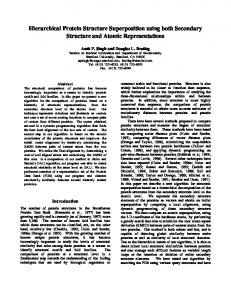
˙ operator yields 0 if the difference is negative.) as follows. (The − PK ˙ i rank M 2 , X (L M 1 (X )[i]) − TopKDist M 1 , M 2 , K (X ) = i=1 . K In order to understand how well the metrics agree on different segments of the ranked lists that they produce, we also define a distance measure over a “window” of the ranked lists. This definition is identical to the previous one, except that instead of looking at the top K according to the first measure, we look at collections in a specific window. In this case, we cannot omit downward displacements, since omitting them would make windows in the lower segments of the list appear closer. For the example in Figure 7, the average distance for a window of size 3, starting at position 2 (i.e., covering collections B, C, and D), is given by (1 + 1 + 1)/3 = 1. Formally, P I +K −1 |rank M 2 , X (L M 1 (X )[i]) − i| . WindowDist M 1 , M 2 , I, K (X ) = i=I K Notice that the ranked lists we have seen so far have been generated by picking an arbitrary collection X , and arranging all other collections by their similarity to it. Thus, in order to be able to compare two measures, we average the distances we compute over all possible choices for X . We note that the variance in the results across the different choices for X is fairly small. Figure 8 shows the average rank displacement in the top K list for various measures with respect to RGM, as a function of K . Notice that the average ACM Transactions on Information Systems, Vol. 21, No. 1, January 2003.

Exploiting Hierarchical Domain Structure

•

83

displacement for the Naive measure, even for the top 10, is as much as 40, which is about 10% of the size of the entire corpus. This result means, informally, that the collections that RGM considers the top 10 would be, on average, around the 40th or 50th position under the Naive measure, a very significant difference! On the other hand, all the Genealogy measures are bunched around the bottom of the graph, with even their peak displacement being well under 20. In fact, for the top 10 list, the average displacement between RGM and OGM is just 1.42. This result means that RGM and OGM agree very well on what the most similar collections to a target collection X are. For the BGM family, as the value of β decreases, the displacement starts getting larger and larger, but it is still much smaller than the displacement of GCSM and that of the Naive measure. It is important to realize that this graph only compares measures against RGM. For example, the displacement between the GCSM and the Naive measure is not given by the difference between the curves corresponding to them on this graph. Also notice that all the curves have roughly the same shape, rising for a while and then dropping off as K increases. This behavior is illustrated better by Figure 9(a), which shows the average rank displacement, in a sliding window of size 10, of all measures with respect to RGM. The general shape of the curves tells us that, for all the measures, there is greater agreement at the beginning and the end of the list than in the middle: there are a few collections that are clearly the most similar and a few that are clearly the most dissimilar. These collections are more easily identified by all the measures and, therefore, the measures agree more in the beginning and the end. Figure 9(b) plots a similar graph, this time comparing the various measures to OGM using a sliding window. Once again, we notice that the Naive measure produces results that are extremely different from the results produced by OGM. For BGM, the distance from OGM gets larger as β decreases, which is to be expected since OGM has β = 1. But the rankings appear much less sensitive to β at the beginning and the end of the ranked lists. We also see that the curve for RGM lies between the curves for β = 0.6 and β = 0.8. Again note that this result does not mean that RGM behaves as BGM with β = 0.7. All it means is that RGM is as different from OGM as BGM with β = 0.7. These graphs establish conclusively that using a hierarchy makes a significant difference to the similarity rankings that are generated. We also conclude that GCSM is rather different from the Genealogy measures, a fact that we attribute to GCSM’s use of many-to-many matches. BGM is sensitive to the specific choice of β, but the sensitivity is much lower at the top and the bottom of the lists. Thus the choice of β is not too critical if one is trying to identify clearly similar or dissimilar collections. RGM and OGM are extremely similar at the top of the list, which is to be expected in this domain. Our data set does not have any multiplicity at the leaf level since it was rarely the case that a student repeated a course and ended up with the same grade. Nevertheless, the presence of a lot of multiplicity at the higher levels illustrates the important role that its interpretation plays in producing similarity values. ACM Transactions on Information Systems, Vol. 21, No. 1, January 2003.

84

•

P. Ganesan et al.

Fig. 9. WindowDist10 with respect to (a) RGM and (b) OGM. ACM Transactions on Information Systems, Vol. 21, No. 1, January 2003.

Exploiting Hierarchical Domain Structure

•

85

Fig. 10. A sample question.

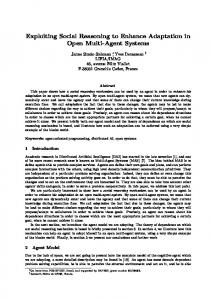
5.2 Matching Human Intuition In order to understand how well the various measures match human intuition, we performed user studies on two different sets of people. Some of the important issues in the design of the study were the following. —The users needed to be familiar with the domain from which the collections were drawn. With this in mind, we chose two different domains: the supermarket domain (with each collection being a bag of grocery items) and the course transcript domain introduced in Section 5.1. —It was not reasonable to expect users to come up with absolute similarity scores between collections. Instead we asked users to rank two collections according to their similarity to a given third collection. —The collections needed to be reasonably small in order to keep the questions tractable. Fortunately, even collections with a small number of distinct elements proved sufficient to test the validity of the premises underlying the different measures. The questions in the user study were chosen to highlight the differences between the various metrics. We cannot claim that our distribution of questions across various collection characteristics exactly resembles the distribution in a real-world application; however, we attempted to maintain a uniform spread across all collection characteristics while continuing to keep the questions relatively easy to understand. Figure 10 shows a sample question from our user study. It shows the purchases of a “query” customer Q and two other customers A and B, along with the product hierarchy associated with their purchases. The objective was to identify which of A and B was more similar to Q. The users were also offered two other choices: that both A and B are equally similar to Q, or that they cannot answer the question intuitively. The latter choice was important in order to not force people to pick one of A and B when neither appeared to be a conclusive winner over the other. In the question shown in Figure 10, a large ACM Transactions on Information Systems, Vol. 21, No. 1, January 2003.

86

•

P. Ganesan et al. Table III. Percentage User Agreement with Similarity Metrics

Qn# 1 2 3 4 5 6 7 8 9 Overall

Jaccard’s 100 0 3 16 0 0 94 94 42 38

EMD 100 100 91 16 16 62 3 94 54 59

GCSM 100 100 91 76 82 0 3 94 4 61

OGM 100 100 91 76 82 0 94 94 4 71

PGM 100 100 91 16 16 38 94 94 54 67

BGM(β = 0.8) 100 100 91 76 82 62 94 94 42 82

RGM 100 100 91 76 82 38 94 94 54 81

majority of the users believed that A was more similar, a conclusion that cannot be arrived at using traditional similarity measures, or using metrics such as Earth-mover’s distance (EMD). We provide a detailed analysis of the reasons underlying the inapplicability of EMD in the extended version of our article [Ganesan et al. 2002]. The test was designed to be immune to the sequence in which questions were posed to the user, so that answering earlier questions did not bias the users towards a specific answer for the later questions. We performed our study on two different sets of users in order to establish statistical validity. One set consisted of 37 people, all of whom had a knowledge of computer science. The second set consisted of a smaller group of 15 people from nontechnical professions. The results of the two studies exhibited extremely high correlation, establishing that the technical background of the test audience had no impact on the results. We describe only the larger-scale study here. Table III shows the percentage of users who agreed with the conclusion that would be reached by each of the listed metrics, for each of nine questions, and the overall agreement with the various metrics. For example, line 5 of Table III shows the results of the studies on the question shown in Figure 10. Of the users polled, 82% chose answer (a), and 16% chose (c). As we can see from the table, GCSM, OGM, BGM, and RGM agree with the majority of the users, whereas EMD and PGM agree with the minority opinion. Jaccard’s picks option (b) which was not chosen by any of the users. From this table, we see that Jaccard’s coefficient, EMD, GCSM, and PGM all predict conclusions that are contrary to the opinion of a majority of the users in at least three of the nine test cases. OGM contradicts the users in two cases, whereas BGM and RGM are the only two metrics that find sizable support for their conclusions in all the cases. This is also reflected in the bottom line, where we see that the overall support for BGM and RGM is significantly higher than that for the other metrics. We also observe that the “bottom line” only gets better if we remove the noise introduced by a few users arriving at conclusions different from the vast majority of the users. Space constraints prevent reporting all our results, but briefly, the following conclusions were drawn from the study. —Using the hierarchy is definitely an improvement over a naive approach, and more intuitive similarity results are obtained. ACM Transactions on Information Systems, Vol. 21, No. 1, January 2003.

Exploiting Hierarchical Domain Structure

•

87

—GCSM does not perform as well as the Genealogy measures in these domains. —There is significant agreement with both BGM and RGM and, in cases where BGM and RGM offer different conclusions, the users are divided on what the right conclusion is. —For BGM, the study established that β values of 0 and 1 (OGM and PGM, respectively) are both unsatisfactory. Again, application semantics would determine the exact value of β although the reasonably low sensitivity to β in our experiments in Section 5.1 suggests that a β value around 0.5 is reasonable. —Using different hierarchies on the same domain leads to different notions of similarity. Comparing the same bags, while superimposing different hierarchies on them, leads to different conclusions. The hierarchy that an application imposes thus enables it to “define” what is meant by the term “similar.” 6. RELATED WORK The use of a hierarchy on attributes is a special case of exploiting general relationships between attributes in order to compute similarity. The SMART system [Salton 1968] was one of the earliest to suggest and use such relationships, and the same idea is also explored in Lustig [1967]. Both works exploit statistical correlations between keywords in computing relevance of documents to queries. Soergel [1967] provides a theoretical framework in which to describe different similarity measures, and proposes and analyzes a number of similarity measures that may be adapted to using a hierarchy by employing our techniques. There have been attempts to improve traditional cosine similarity, as well as address data sparsity, using dimensionality-reduction techniques such as Latent Semantic Indexing (LSI) [Deerwester et al. 1990]. This technique actually shows some improvement in the quality of the similarity scores, since it tries to infer latent relationships between dimensions. Such techniques have also been tried in collaborative filtering [Sarwar et al. 2000] but it appears somewhat unclear as to whether it actually improves recommendation quality. Notice that using a domain hierarchy is actually an implicit form of dimension reduction, because the hierarchy implies that all elements are not orthogonal to each other. On the other hand, our techniques explicitly define the relationship between the different dimensions, whereas LSI infers the relationships from the corpus. Ioannidis and Poosala [1999] study the problem of computing distance between bags of real numbers and propose a matching-based metric called MAC that bears some resemblance to our BGM. MAC was designed to address many of the same concerns that we outlined but does not map to a clear semantics when we apply it to work with hierarchies, perhaps because it was designed to work with sets of numbers. It also requires the setting of two tuning parameters that make a significant difference to the numbers computed by the algorithm. Furthermore, it is formulated as a graph-theoretic problem and could be expensive to compute. Nonetheless, the motivations behind its design are very similar to ours and Ioannidis and Poosala [1999] explain the shortcomings of alternative metrics at some length. ACM Transactions on Information Systems, Vol. 21, No. 1, January 2003.

88

•

P. Ganesan et al.

Yet another class of distance measures is edit distance [Sankoff and Kruskal 1983], wherein the distance between two structures is measured by the cost of the edit operations needed to transform one structure to the other. Algorithms for finding the optimal edit script exist for various types of structures, and for various sets of edit operations. Computing the optimal edit distance between unordered trees, even with simple edit operations, is NP-complete [Shasha and Zhang 1997]. In addition, edit distance does not give us the freedom to deal with nuances of intercollection similarity, such as handling multiple occurrences. Information-theoretic measures such as the expected mutual information and information radius [van Rijsbergen 1979; Sibson 1972] have also been used as measures of similarity (or dissimilarity) in classification and clustering applications. van Rijsbergen [1979] discusses how these measures may be used in probabilistic models in order to capture correlations between different terms occurring in the corpus. However, these measures are more useful as a means of measuring similarity between elements rather than in dealing with sets or bags of elements. Again, there is no easy way to support different semantics for multiple occurrences. There have been quite a few attempts to use word hierarchies such as WordNet [Miller et al. 1990] in information retrieval. In Rada et al. [1989], the semantic similarity between two words is defined as the weight of the path between the words, which is similar to our definition of the LCA of two leaves. Other works [Lee and Kim 1993; Kim and Kim 1990] have also used this “conceptual distance” measure for information retrieval. There are also other information-based measures based on the same hierarchy [Resnick 1995] that can be used for word similarity. Richardson and Smeaton [1995] compare the efficacy of different word-similarity measures in computing query—document similarity. All these works are focused on query—document similarity and do not generalize to intercollection similarity. Richardson and Smeaton [1995] also discuss the issue of generating edge weights for the concept graphs, which could find use in our work in generating edge weights for our hierarchy, as discussed in the full version of our article [Ganesan et al. 2002]. Our definition of the dot product between the unit vectors is also similar to the hypermetric generated by hierarchical classification [Sneath and Sokal 1973]. This connection to classification is more coincidental than directly relevant, since a hypermetric is a natural consequence of any hierarchy, whether it is given a priori or generated by hierarchical classification. The measure we use is not the natural hypermetric on the hierarchy, which is simply the distance to the lowest common ancestor, but a normalized version of the depth of the lowest common ancestor. Scott and Matwin [1998] study the use of a hypernym density representation instead of a bag-of-words representation in text classification and report improvements for corpora with a reasonable amount of diversity. de Buenaga Rodr´ıguez et al. [1997] also report improvements in text classification when using WordNet to enhance neural network learning algorithms. But neither of these works uses a direct similarity measure based on the hierarchy. Concept hierarchies have frequently been used in data mining. They have been used to mine multilevel association rules [Han and Fu 1995; Srikant ACM Transactions on Information Systems, Vol. 21, No. 1, January 2003.

Exploiting Hierarchical Domain Structure

•

89

and Agrawal 1995] and to improve knowledge discovery in textual databases [Feldman and Dagan 1995]. Neither of these two applications is directly related to computing similarity using hierarchies. There has also been work on computing similarity between attributes, and inferring attribute hierarchies in tables by using learning techniques on the data in the tables [Das et al. 1998]. This problem may be viewed as being a dual to ours, as it tries to infer a hierarchy from the data rather than the other way round. There are other classes of methods used to compute similarity between collections that exploit the structure between collections. For example, Bollacker et al. [1998] and Jeh and Widom [2001] use the link structure of research papers to compute similarity between them. Melnik et al. [2002] use a graph-theoretic algorithm called Similarity Flooding to identify mappings between schemas. Such methods are not directly related to our work, except they may perhaps be used to solve the same overall problem. 7. CONCLUSIONS We proposed exploiting hierarchical domain structure to compute similarity between collections. We defined similarity measures that use the hierarchy, showed why traditional measures, as well as some of our own measures, often have unsatisfactory semantics, and suggested refinements that provide good semantics for intercollection similarity. We performed empirical comparisons of our measures with traditional similarity measures, and showed that using the hierarchy makes a large difference, both in terms of the values that are produced, and in terms of ranked lists of collections similar to a given collection. We have reported the findings of a user study justifying our belief that our measures generate results that are closer to human intuition than the traditional similarity measures. We are currently in the process of building recommender systems using the measures introduced in this article, and using the hierarchy in other portions of the recommender system. Preliminary results are encouraging, and seem to provide higher-quality recommendations than the simple Pearson-correlationbased, nearest neighbor approaches. APPENDIX A. BGM DETAILS AND PROOF OF THEOREMS Recall from Section 4.1 that, for trees where all leaves are at the same level, the BGM algorithm operates in phases. In the first phase, it looks only for exact matches between leaves. In the second phase, it looks for pairs of leaves with a common parent, in the third phase, pairs of leaves with a common grandparent, and so on. This strategy is guaranteed to produce the optimal score. The strategy for the general case, where we have leaves at different depths and different leaf weights, is a generalization of the strategy outlined above. The key idea is to generate leafsim values in decreasing order of optleafsim∗ W , using a generalization of the multiphase approach. This order is computed in a preprocessing step, and does not have to be generated for each individual ACM Transactions on Information Systems, Vol. 21, No. 1, January 2003.

90

•

P. Ganesan et al.

similarity computation. We now prove that this strategy does compute the BGM score according to the optimal order. (We take all weights to be 1, for simplicity.) THEOREM 1. If the BGM algorithm looks for matches in decreasing order of their optleafsim contribution, then it computes the BGM score according to the optimal order. PROOF. We observe that BGM is exactly identical to OGM in terms of the set of possible matches that every leaf has, except that some of the match value contributions are reduced by multiplication by some power of β. For any leaf l 1 belonging to tree T1 , there is an associated set matchT1 ,T2 (l 1 ). The optleafsim value that we attach to a match of l 1 is the same irrespective of which element of the set to which we match l 1 . From this fact, it follows that the number of matches for which the match value is reduced (as compared to the optimistic match value) is independent of the sequence in which we match leaves from the first tree T1 . Consequently, ensuring that we consider matches in decreasing order of optleafsim values ensures that we always reduce the smallest possible optleafsim value at every stage and, therefore, provides us with the BGM score according to the optimal order. THEOREM 2. If l is the total number of leaves in T1 and T2 , h is the maximum depth of the hierarchy, and b is the maximum branching factor in T2 , the worstcase computational complexity of the algorithm is O(lh(h + log b). PROOF. We first observe that, unlike the OGM algorithm, we need to maintain state in each of the leaves keeping count of how many times the leaf has been matched so far. When trying to choose from a set of possible matches the leaf that has been matched the fewest number of times so far, it would be much too expensive to check each of the possible matches and then choose the minimally matched leaf. Instead, at each internal node of T2 , we maintain a priority queue of its children, prioritized by the least number of matches of any leaf in the subtree of each of the children. As leaves are matched during the algorithm, the priority queues need to be updated to reflect the changes. Our observation is that we will never need to update more than one priority queue for any additional match that we make. This is because the key values in the priority queues always increase by one, meaning that if the minimum key value k in a priority queue increases to k + 1 and necessitates an update to the priority queue, the minimum value in the priority queue continues to be k (if it is greater than k, then no update would have been necessary). Thus the minimum value of the priority queue did not change and, therefore, none of the priority queues above this node will require any updates. From this observation, it is easy to see that the BGM algorithm is bounded by a worst-case complexity of O(lh(h + log b). The cost of traversing down the hierarchy to find a match for a leaf and updating the priority queue is captured by h + log b. For each leaf, we attempt to match it at most h times, once at each level of its ancestors, due to which we get the factor lh. ACM Transactions on Information Systems, Vol. 21, No. 1, January 2003.

Exploiting Hierarchical Domain Structure

•

91

B. FORMAL DEFINITION OF RGM Recall Section 4.2. For any tree T and any node n in T , let CT (n) be the set of all children of n in T . Let WT (k) be the weight of node k in tree T . We explain shortly how to compute WT (k), given our original weight function W which is defined only for the leaves of trees. Let C1 and C2 be the two collections under comparison, and let T1 and T2 be their associated trees, as usual. We first define the weights to be associated with all the nodes in tree T2 . We then define the weights for all the nodes in T1 . WT2 (n) = W (n) if n is a leaf of T2 X = WT2 (c) if n is an internal node of T2 c∈CT2 (n)

= ∞ otherwise. We have defined the weights of nodes not in T2 to be ∞ for notational convenience. WT1 (n) = W (n) if n is a leaf of T1   X = min  WT1 (c), WT2 (n)

if n is an internal node of T1

c∈CT2 (n)

= 0

otherwise.

For any internal node in T1 , its weight is determined both by the sum of the weights of its children in T1 , say p, and by the weight of the same node in T2 , say q. Although we have chosen to use min( p, q) as our weight, we could, in general, use any function, although functions that return a value between p and q make the most sense. The effect of this choice was discussed in Section 4.3. Let simT1 ,T2 (n) denote the similarity value “at” a node n in tree T1 . The similarity between the two trees sim(T1 , T2 ) is given by sim(T1 , T2 ) = simT1 ,T2 (root(T1 )). For all nodes n in T1 , we define: simT1 ,T2 (n) = optleafsimT1 ,T2 (n) if n is a leaf (defined in Section 4.1.1) P c∈CT1 (n) W T1 (c) ∗ simT1 ,T2 (c) P = if n is an internal node c∈CT (n) W T1 (c) 1

REFERENCES BOLLACKER, K., LAWRENCE, S., AND GILES, C. L. 1998. CiteSeer: An autonomous Web agent for automatic retrieval and identification of interesting publications. In Proceedings of the Second International Conference on Autonomous Agents, 116–123. BREESE, J. S., HECKERMAN, D., AND KADIE, C. 1998. Empirical analysis of predictive algorithms for collaborative filtering. In Proceedings of the Fourteenth Annual Conference on Uncertainty in Artificial Intelligence. CHAKRABARTI, K., GAROFALAKIS, M. N., RASTOGI, R., AND SHIM, K. 2000. Approximate query processing using wavelets. In Proceedings of VLDB 2000, 111–122. ACM Transactions on Information Systems, Vol. 21, No. 1, January 2003.

92

•

P. Ganesan et al.

DAS, G., MANNILA, H., AND RONKAINEN, P. 1998. Similarity of attributes by external probes. In Proceedings of Knowledge Discovery and Data Mining (KDD), 23–29. ´ DE BUENAGA RODR´IGUEZ, M., GOMEZ -HIDALGO, J. M., AND D´IAZ-AGUDO, B. 1997. Using WordNet to complement training information in text categorization. In Proceedings of the Second International Conference on Recent Advances in Natural Language Processing. DEERWESTER, S., DUMAIS, S. T., FURNAS, G. W., LANDAUER, T. K., AND HARSHMAN, R. 1990. Indexing by latent semantic indexing. J. Amer. Soc. Inf. Sci. 41, 6, 391–407. FELDMAN, R. AND DAGAN, I. 1995. Knowledge discovery in textual databases. In Proceedings of KDD-95. GANESAN, P., GARCIA-MOLINA, H., AND WIDOM, J. 2002. Exploiting hierarchical domain structure to compute similarity. Tech. Rep., Available at http://dbpubs.stanford.edu/pub/2001-27. GOLDBERG, D., NICHOLS, D., OKI, B. M., AND TERRY, D. 1992. Using collaborative filtering to weave an information tapestry. Commun. ACM 35, 12, 61–70. GOOD, N., SCHAFER, J. B., KONSTAN, J. A., BORCHERS, A., SARWAR, B. M., HERLOCKER, J. L., AND RIEDL, J. 1999. Combining collaborative filtering with personal agents for better recommendations. In Proceedings of AAAI/IAAI. HAN, J. AND FU, Y. 1995. Discovery of multiple-level association rules from large databases. In Proceedings of VLDB ’95, 420–431. IOANNIDIS, Y. E. AND POOSALA, V. 1999. Histogram-based approximation of set-valued queryanswers. In Proceedings of VLDB 1999, 174–185. JEH, G. AND WIDOM, J. 2001. Simrank: A measure of structural-context similarity. Tech. Rep. Stanford University. Available at http://dbpubs.stanford.edu/pub/2001-41. JOSHI, A. AND KRISHNAPURAM, R. 2000. On mining Web access logs. In ACM SIGMOD Workshop on Research Issues in Data Mining and Knowledge Discovery, 63–69. KIM, Y. AND KIM, J. 1990. A model of knowledge based information retrieval with hierarchical concept graph. J. Doc. 46, 2, 113–116. LEE, J. AND KIM, M. 1993. Information retrieval based on a conceptual distance in is-a heirarchy. J. Doc. 49, 2, 188–207. LUSTIG, G. 1967. A new class of association factors in mechanized information storage, retrieval and dissemination. In F. I. D./I. F. I. P. Joint Conference (Rome). MCGILL, M. J. 1983. Introduction to Modern Information Retrieval. McGraw-Hill, New York. MELNIK, S., GARCIA-MOLINA, H., AND RAHM, E. 2002. Similarity flooding: A versatile graph matching algorithm. In Proceedings of ICDE 2002. MILLER, G. R. B. FELLBAUM, C., GROSS, D., AND MILLER, K. 1990. Introduction to WordNet: An on-line lexical database. J. Lexicog. 3, 4, 234–244. NASRAOUI, O., FRIGUI, H., JOSHI, A., AND KRISHNAPURAM, R. 1999. Mining Web access logs using relational competitive fuzzy clustering. In Proceedings of the Eighth International Fuzzy Systems Association World Congress—IFSA 99 (Taipei). OPD. The Open Directory Project. Available at http://dmoz.org/. RADA, R., MILI, H., BICKNELL, E., AND BLETTNER, M. 1989. Development and application of a metric on semantic nets. IEEE Trans. Syst. Man Cybern. 19, 1, 17–30. RESNICK, P. 1995. Using information content to evaluate semantic similarity in a taxonomy. In Proceedings of the International Joint Conference on Artificial Intelligence (IJCAI), 448–453. RESNICK, P., IACOVOU, N., SUSHAK, M., BERGSTROM, P., AND RIEDL, J. 1994. Grouplens: An open architecture for collaborative filtering of netnews. In Proceedings of the Computer Supported Collaborative Work Conference. RICHARDSON, R. AND SMEATON, A. F. 1995. Using WordNet in a knowledge-based approach to information retrieval. In Proceedings of the Seventeenth BCS-IRSG Colloquium on Information Retrieval. RUBNER, Y., TOMASI, C., AND GUIBAS, L. J. 1998. The earth mover’s distance as a metric for image retrieval. Tech. Rep. STAN-CS-TN-98-86, Stanford University. SALTON, G. 1968. Automatic Information Organization and Retrieval. McGraw-Hill, New York. SALTON, G. AND BUCKLEY, C. 1988. Term-weighting approaches in automatic text retrieval. Inf. Process. Manage. 24, 5, 513–523. SANKOFF, D. AND KRUSKAL, J. B. 1983. Macromolecules: The Theory and Practice of Sequence Comparison. Addison-Wesley, Reading, MA. ACM Transactions on Information Systems, Vol. 21, No. 1, January 2003.

Exploiting Hierarchical Domain Structure

•

93

SARWAR, B., KARYPIS, G., KONSTAN, J., AND RIEDL, J. 2000. Application of dimensionality reduction in recommender system—a case study. In Proceedings of the ACM WebKDD 2000 Workshop. SARWAR, B., KARYPIS, G., KONSTAN, J., AND RIEDL, J. 2001. Item-based collaborative filtering recommendation algorithms. In Proceedings of the Tenth International WWW Conference. SARWAR, B. M., KONSTAN, J. A., BORCHERS, A., HERLOCKER, J. L., MILLER, B. N., AND RIEDL, J. 1998. Using filtering agents to improve prediction quality in the GroupLens Research collaborative filtering system. In Proceedings of the ACM Conference on Computer-Supported Cooperative Work (CSCW). SCOTT, S. AND MATWIN, S. 1998. Text classification using WordNet hypernyms. In Proceedings of the Use of WordNet in Natural Language Processing Systems. Association for Computational Linguistics. SHASHA, D. AND ZHANG, K. 1997. Approximate tree pattern matching. In Pattern Matching Algorithms, Oxford University Press, New York. SHIVAKUMAR, N. AND GARCIA-MOLINA, H. 1995. Scam: A copy detection mechanism for digital documents. In Proceedings of the Second International Conference in Theory and Practice of Digital Libraries. SIBSON, R. 1972. Order invariant methods for data analysis. J. Roy. Stat. Soc. 34, 3, 311–349. SNEATH, P. AND SOKAL, R. 1973. Numerical Taxonomy. W. H. Freeman, San Francisco. SOERGEL, D. 1967. Mathematical analysis of documentation systems. An attempt at a theory of classification and search request formulation. Inf. Stor. Retrieval 3, 3, 129–173. SRIKANT, R. AND AGRAWAL, R. 1995. Mining generalized association rules. In Proceedings of VLDB ’95, 407–419. STREHL, A., GHOSH, J., AND MOONEY, R. 2000. Impact of similarity measures on Web-page clustering. In Proceedings of the AAAI Workshop on AI for Web Search. VAN RIJSBERGEN, C. J. 1979. Information Retrieval. 2nd ed., Butterworths, London. Received February 2002; revised November 2002; accepted November 2002

ACM Transactions on Information Systems, Vol. 21, No. 1, January 2003.