arXiv:1503.04144v2 [cs.CV] 16 Mar 2015
Exploiting Image-trained CNN Architectures for Unconstrained Video Classification Shengxin Zha Northwestern University Evanston IL USA
Florian Luisier, Walter Andrews Raytheon BBN Technologies Cambridge, MA USA
[email protected]
{fluisier,wandrews}@bbn.com
Nitish Srivastava, Ruslan Salakhutdinov University of Toronto {nitish,rsalakhu}@cs.toronto.edu
Abstract
Video level CNN features
Kernel SVM Spatiotemporal pooling and normalization
We conduct an in-depth exploration of different strategies for doing event detection and action recognition in videos using convolutional neural networks (CNNs) trained for image classification. We study different ways of performing frame calibration, spatial and temporal pooling, feature normalization, choice of CNN layer as well as choice of classifiers. Making judicious choices along these dimensions led to a very significant increase in performance over more naive approaches that have been used till now. We illustrate our procedure with two popular CNN architectures which got excellent results in the ILSVRC-2012 and 2014 competitions. We test our methods on the challenging TRECVID MED’14 dataset which contains a heterogeneous set of videos that vary in terms of resolution, quality, camera motion and illumination conditions. On this dataset, our methods, based entirely on image-trained CNN features, can already outperform state-of-the-art non-CNN models based on the best motion-based Fisher vector approach. We further show that late fusion of CNN- and motion-based features brings a tremendous improvement, increasing the mean average precision (mAP) from 34.95% to 38.74%. The fusion approach also matches the state-ofthe-art classification performance on UCF-101 dataset.
Frame Patch CNN feature extraction
Frame t + 1
Frame t
Input videos
Kernel SVM model or event score
CNN feature extraction
Video frames sampling and calibration
Frame patches
Kernel SVM training or testing
CNN feature extraction
Frame t + 2
CNN feature extraction
Video-level CNN features
Frame-level CNN features
Spatiotemporal pooling and normalization
Figure 1. Overview of the proposed video classification pipeline.
age classification pipeline consists of first extracting multiple carefully engineered local feature descriptors (e.g., SIFT [18] or SURF [2]), and then encoding them through a bag-of-words (BoW) [3] or Fisher vector (FV) [22, 23] representation, and finally training a classifier (e.g., support vector machines–SVMs) on top of the encoded features. The main limitation of the transposition of the standard image classification approach to video is the lack of exploitation of motion information. This shortcoming has been addressed by extracting descriptors from spatiotemporal interest points ( e.g., [15, 4, 35, 16, 34]) or along estimated motion trajectories (e.g., [31, 11, 9, 32, 33]). The success of deep convolutional neural networks (CNN) on the ImageNet large-scale visual recognition challenge1 has generated considerable attention in the computer vision research community. Since the publication of the winning model of the ImageNet 2012 challenge [13], CNNbased approaches have been shown to achieve state-of-the-
1. Introduction The huge volume of videos that are nowadays routinely produced by consumer cameras and shared across the web calls for effective video classification and retrieval tools. One of the most straightforward approaches considers a video as a set of images (video frames) and relies on techniques designed for image classification. This standard im-
1 http://www.image-net.org
1
art on many challenging image datasets. For instance, CNN-based features extracted from pre-trained ImageNet models have been successfully transferred to the PASCAL VOC dataset and used as a mid-level image representation [6]. They have been shown to outperform the stateof-the-art for action and object classification, while achieving promising results for object and action localization [20]. An evaluation of off-the-shelf CNN features applied to visual classification and visual instance retrieval has been recently conducted on several image datasets in [25]. The main observation from these experiments is that the CNNbased features achieve superior performance compared to the approaches based on the most successful hand-designed features. Recently, CNN architectures trained on videos have emerged, with the objective of capturing and encoding motion information. The 3D CNN model proposed in [10] achieves superior performance in human action recognition compared to baseline methods. The spatiotemporal CNN model described in [12] shows consistently better results for large-scale video classification compared to strong handcrafted feature-based approaches. The two-stream convolutional network proposed in [26] combines a CNN model trained on appearance frames with a CNN model trained on stacked optical flow features to match the performance of hand-crafted spatiotemporal features. In this paper, we propose an efficient procedure to exploit off-the-shelf image-trained CNN architectures for video classification. Figure 1 shows the overall video classification pipeline. Our contributions are the following: • We discuss each step of the proposed video classification pipeline, including the choice of CNN layers, the video frame sampling and calibration, the spatial and temporal pooling, the feature normalization, and the choice of classifier. All our design choices are supported by extensive experiments on the TRECVID MED’14 video dataset. • We provide extensive comparisons between the CNNbased approach and some state-of-the-art static and motion-based Fisher vector techniques, showing that the CNN-based approach can outperform the latter. • We show that integrating motion information with simple late fusion considerably improves classification performance. Our work is closely related to other research and development efforts towards the efficient use of CNN for video classification. While it is now clear that CNN-based approaches outperform most state-of-the-art handcrafted features for image classification [25], it is not yet obvious that this holds true for video classification. Moreover, there seems to be mixed conclusions regarding the benefit of
Events E021-E030 Attempting a bike trick Cleaning an appliance Dog show Giving directions Marriage proposal Renovating a home Rock climbing Town hall meeting Winning a race w/o a vehicle Working on a metal crafts project
Events E031-E040 Beekeeping Wedding shower Non-motorized vehicle repair Fixing a musical instrument Horse riding competition Felling a tree Parking a vehicle Playing fetch Tailgating Tuning a musical instrument
Table 1. TRECVID 2014 pre-specified events.
training a spatiotemporal vs. applying an image-trained CNN architecture on videos. Indeed, while Ji et. al. [10] observe a significant gain using 3D convolutions over the 2D CNN architectures and Simonyan et. al. [26] obtain significant gains over an appearance based 2D CNN using optical flow features alone, Karpathy et. al. [12] report only a moderate improvement. Although the specificity of the considered video datasets might play a role, the way the 2D CNN architecture is exploited for video classification is certainly the main reason behind these contradictory observations. The additional computational cost of training on videos is also an element that should be taken into account when comparing the two options. Prior to training a spatiotemporal CNN architecture, it thus seems legitimate to fully exploit the potential of image-trained CNN architectures. Obtained on a highly heterogeneous video dataset, we believe that our results can serve as a strong 2D CNN baseline against which to compare CNN architectures specifically trained on videos.
2. Video Dataset and Performance Metric All the configuration experiments presented in this paper have been conducted on the official TRECVID MED’14 video dataset [21]. Parameter tuning is done on training set. This dataset consists of: • A training set of 4,992 unlabeled background videos. This set of videos are used as the negative examples in all our experiments. • A training set of 2,991 positive and near-miss videos. The set of positive videos contains about 100 examples for each of the 20 pre-specified events (see Table 1). The set of near-miss videos contains about 50 nearmiss videos for each of the 20 pre-specified events. In all our experiments, we treated the near-miss videos as negative exemplars. • A test set of 23,953 videos which contains positive and negative instances of the 20 pre-specified events.
Attempting a bike trick
Renovating home
Cleaning appliance
Rock Climbing
Dog Show
Town hall meeting
Giving directions
Marriage Proposal
Winning race without vehicle Working on metal crafts project
Figure 2. Sample frames from the TRECVID MED ’14 dataset.
Contrary to other popular video datasets, such as UCF101 [28] or Hollywood2 [19], the TRECVID dataset is not constrained to any class of videos. It consists of a heterogeneous set of YouTube-like videos of various resolutions, quality, camera motions, and illumination conditions. The TRECVID dataset is thus one of the largest and most challenging dataset for video event detection. Some sample frames are shown in Figure 2. As a retrieval performance metric, we consider the one used in the official TRECVID multimedia event detection task; i.e., mean average precision (mAP) across all events. Let E denote the number of events, Pe the number of positive instances of event e, then mAP is computed as mAP =
E 1 X AP(e), E e=1
(1)
where the average precision of an event e is defined as AP(e) =
Pe 1 X p . Pe p=1 rank(p)
mAP is thus normalized between 0 (low classification performance) and 1 (high classification performance). In this paper, we will report it in percentage value.
3. Deep Convolutional Neural Networks Convolutional neural networks consist of layers of spatially-structured hidden units. Each hidden unit typically looks at a small patch of hidden (or input) units in the previous layer, applies some operation to it and then applies a non-linearity to the result to compute its own state. The hidden layers are stacked together to form a deep network. The basic building blocks are convolution and pooling operations. In a convolution operation, a spatial patch of units is convolved with multiple filters (learned weights) to generate
feature maps. The convolution operation is applied spatially with some stride. A pooling operation takes a spatial patch and computes a summary of that patch for each input channel. This summary is often chosen to be the maximum activation (max pooling) or average activation (average pooling). This pooling operation creates some translation invariance. The hyper-parameters, such as the size of the spatial patch and stride, are tuned on a validation set. At the top of the stack, the spatially organized hidden units are densely connected to a layer of hidden units which eventually connect to the output units. If the aim is to do object recognition, the output layer is a softmax which corresponds to a vector of probabilities of different object classes. The network can be trained with back-propagation to optimize an appropriate objective function depending on the task. Regularizers, such as `2 decay and dropout [29], are effective. The rectified linear activation function is usually used for all hidden units. The structure of deep neural nets enables the hidden layers to learn rich distributed representations of the input images. The densely connected layers, in particular, can be seen as learning a high-level representation of the image by accumulating information from all the spatial locations. We initially developed our work on the winning model of ILSRC-2012 competition by Krizhevsky et. al. [13]. In the recent ILSVRC-2014 competition, the winning model GoogLeNet [30] and the close runner-up model VGG [27] show superior performance over [13], using smaller receptive fields (1×1, 3×3 and 5×5 in [30] and 3×3 in [27]) and more depth (22 layers in [30] and up to 19 layers in [27]). Multi-scale training also improves the image classification performance [27]. We adopt the publicly available pretrained models of [27] and [13] in our system. The proposed approach is generic with respect to CNN architectures. Therefore, it can be adapted to other CNN models as well.
4. Video Classification Pipeline Figure 1 gives an overview of the proposed video classification pipeline. Each component of the pipeline is discussed in the following sections.
4.1. Choice of CNN Layer We have considered the output layer and the last two hidden layers as CNN-based features. The 1,000-dimensional output-layer features, with values between [0, 1], are the posterior probability scores corresponding to the 1,000 classes from the ImageNet dataset. Since our 20 events of interest are different from the 1,000 ImageNet classes, the output-layer features are rather sparse (see Figure 3, left panel). The hidden-layer features are treated as high-level image representations in our video classification pipeline. These features are outputs of rectified linear units (RELUs). Therefore, they are lower bounded by zero but do not have a pre-defined upper bound (see Figure 3 middle and right panels) and thus require some normalization. Several normalizations are discussed in Section 4.5.
4.2. Video Frame Sampling and Calibration Each video clip is uniformly sampled into 50 to 120 frames, depending on the length of the clip. We have explored alternative frame sampling schemes (e.g., based on keyframe detection), but found that they all essentially yield the same performance as uniform sampling. The first layer of the CNN architecture takes 224 × 224 RGB images as input. Instead of rescaling the extracted video frames to 224 × 224, we propose to calibrate every frame to a width of 640 pixels, without altering their aspect ratio. We then extract 10 overlapping square patches from the calibrated frames, as illustrated in Figure 4, and rescale each of them to a size of 224 × 224. Each of these patches is then used as input to the CNN architecture. We thus obtain 10 different outputs for each video frame. In the next section, we discuss a few spatiotemporal pooling strategies.
4.3. Spatial and Temporal Pooling In order to obtain a single video-level feature from the multiple frame-level features, we have investigated several spatiotemporal pooling strategies. Inspired by the spatial pyramid approach developed for bags of features [17], we propose to spatially pool together the CNN features computed on patches centered in the same pre-defined subregion of the video frames. Independent with our work, spatial pooling is also applied in [8, 7, 36] in different ways. We have considered 8 different regions consisting of 1 × 1, 3 × 1 and 2 × 2 partitions of the video frame, as shown in Figure 4. For instance, features from patches 1, 2, 3 in Figure 4 will be pooled together to yield a single feature in region 2 in Figure 4.
1
2
3
4
5/10
6
7
8
9
2 1
4
(a)
5
6
7
8
3
(b)
Figure 4. (a). The 10 overlapping square patches extracted from each video frame. The red patch (centered at location 10) has sides equal to the frame height, whereas the other patches (centered at locations 1-9) have sides equal to half of the frame height. (b). Spatial pyramids (SP). Left: the 1 × 1 spatial partition includes the entire frame. Middle: the 3 × 1 spatial partitions include the top, middle and bottom of the frame. Right: the 2 × 2 spatial partitions include the upper-left, upper-right, bottom-left and bottom-right of the frame.
As observed in Table 2 and 3, concatenating the 8 partitions gives the best performance almost in all CNN layers and SVM choices (up to 6% mAP gain over no spatial pooling), but at the expense of an increased feature dimensionality and consequently, an increased training and testing time. A good trade-off between performance and running time can be achieved by considering the 3 × 1 partitioning. For the pooling itself, we evaluated average and max pooling. We observed a consistent gain (around 1% mAP) for max pooling over average pooling for both spatial and temporal pooling, no matter which CNN layer was used. A possible explanation for this comes from the highly heterogeneous structure of our video dataset. A lot of videos contain frames that can be considered irrelevant or at least less relevant than others; e.g., introductory text and black frames. Hence it is beneficial to use the maximum features response, instead of giving an equal weight to all features.
4.4. Feature Normalization While training a SVM model on top of the CNN output features can give acceptable results without prior normalization, appropriate normalization is essential for the last two layers. Let f ∈ RD denote the original video-level CNN feature vector and ˜ f ∈ RD its normalized version. We have investigated three different normalizations: 1. `1 normalization: ˜ f = f /kf k1 . Such feature normalization did not perform well. It even reduces the classification performance as compared to no normalization. 2. `2 normalization: ˜ f = f /kf k2 . Such feature normalization is typically performed prior to training an SVM model. As observed in Table 2 and 3, the `2 normalization is essential to achieve good performance with the hidden6 and hidden7 layers. p 3. root normalization: ˜ f = f /kf k1 . The root normalization was introduced in [1], where it was shown to
5
6
5
x 10
2
5
x 10
x 10
2.5
1.8 5
4
3
2
2
1.4
Number of counts
Number of counts
Number of counts
1.6
1.2 1 0.8 0.6 0.4
1.5
1
0.5
1 0.2 0
0
0.1
0.2
0.3
0.4
0.5
0.6
0.7
0.8
0.9
1
0
0
10
20
30
Value
40
50
60
70
80
0
0
5
10
Value
15
20
25
30
35
Value
Figure 3. Distribution of values for the output layer and the last two convolutional layers of the CNN architecture obtained on the TRECVID MED’14 video dataset: Left: output. Middle: hidden6. Right: hidden7.
improve the performance of SIFT descriptors. When applied to the CNN output layer, we observed a small gain over the `2 normalization when using the CNN architecture from [13]; it yields essentially the same performance when using CNN architecture from [27] (see Table 2 and 3). Yet, we noticed a drop in performance when the root normalization is applied to the hidden6 and hidden7 layers. In summary, we recommend a root normalization for the CNN output layer and an `2 normalization for the hidden6 and hidden7 layers.
4.5. Choice of Classifier We ran all our experiments using SVM classifiers. We trained one SVM model for each event following the TRECVID MED’14 training rules; i.e., excluding the positive and near-miss examples of the other events. We observed that kernel SVM consistently outperforms linear SVM regardless of what CNN layer or which type of normalization was used. For the output layer, which essentially behaves like a histogram-based feature, the best results are achieved with a χ2 kernel. For the hidden6 and hidden7 layers, the best performance is obtained with a Gaussian radial basis function (RBF) kernel. As shown in Table 2 and 3, kernel SVM outperforms linear SVM by about 5% mAP when all other model configurations remain the same.
5. Experiments We design our experiments to compare CNN-based features with Fisher vectors over state-of-the-art static and spatiotemporal features. We also show that the late fusion of image-trained CNN features and motion-based Fisher vectors brings significant gain over both features. Moreover, we compare our CNN-based approach to other CNN-based approaches in video event detection and action recognition datasets.
Layer output output output output output output output hidden6 hidden6 hidden6 hidden6 hidden6 hidden7 hidden7 hidden7 hidden7 hidden7
Dim. 1,000 1,000 8,000 8,000 8,000 1,000 3,000 4,096 32,768 32,768 32,768 12,288 4,096 32,768 32,768 32,768 12,288
SP none none SP8 SP8 SP8 none SP3 none SP8 SP8 SP8 SP3 none SP8 SP8 SP8 SP3
Norm. none root `2 root root root root `2 `2 root `2 `2 `2 `2 root `2 `2
SVM kernel linear linear linear linear χ2 χ2 χ2 linear linear linear RBF RBF linear linear linear RBF RBF
mAP 17.47% 15.90% 22.01% 22.04% 27.22% 21.54% 26.20% 22.11% 23.21% 21.13% 28.20% 27.81% 21.45% 25.01% 23.72% 29.41% 28.14%
Table 2. Various configurations of video classification based on the CNN architecture from [13]. The spatiotemporal pooling method for all results shown in this table is max-pooling. SP8 and SP3 refers to the 1 × 1 + 3 × 1 + 2 × 2 and 3 × 1 spatial pyramids (SPs), respectively.
5.1. Fisher Vectors A very effective approach to event detection from videos is to first extract multiple low-level feature descriptors across the entire video and encode them into a fixed-length video-level Fisher vector (FV). A Fisher vector is a generalization of the popular bag-of-words approach that encodes not only the zero-order statistics of the descriptors distribution but also the first- and second-order statistics. The Fisher vector encoding procedure is summarized below [23]: • Learn a Gaussian mixture model (GMM) on low-level descriptors extracted from a generic set of unlabeled videos. • Compute the gradients of the log-likelihood of the
Layer output output output output output hidden6 hidden6 hidden6 hidden6 hidden7 hidden7 hidden7 hidden7
Dim. 1,000 8,000 8,000 8,000 1,000 4,096 32,768 32,768 32,768 4,096 32,768 32,768 32,768
SP none SP8 SP8 SP8 none none SP8 SP8 SP8 none SP8 SP8 SP8
Norm. root `2 root root root `2 `2 root `2 `2 `2 root `2
SVM kernel Linear Linear Linear χ2 χ2 Linear Linear Linear RBF Linear Linear Linear RBF
mAP 19.46% 25.88% 25.67% 31.24% 25.30% 25.37% 28.31% 26.27% 33.54% 25.08% 29.7% 26.57% 34.95%
Table 3. Various configurations of video classification based on the CNN architecture from [27], with max spatiotemporal pooling.
GMM (known as the score function) with respect to the GMM parameters. The gradient of the score function with respect to the mixture weight parameters encodes the zero-order statistics. The gradient with respect to the Gaussian means encodes the first-order statistics, while the gradient with respect to the Gaussian variance encodes the second-order statistics. • Concatenate the score function gradients into a single vector and apply a signed square rooting on each FV dimension (power normalization) followed by a global `2 normalization. As low-level features, we considered both the standard D-SIFT descriptors [18] and the more sophisticated motionbased improved dense trajectories (IDT) [33]. For both, we selected the parameters giving us the best mAP performance on the validation set, in the same way as we did for the CNN-based features, to allow a fair comparison between the two approaches. For the SIFT descriptors, we opted for multiscale (5 scales) and dense (stride of 4 pixels in both spatial dimensions) sampling, root normalization [1] and spatiotemporal pyramid pooling. For the IDT descriptors, we concatenated histogram of oriented gradients [4], histogram of flow [5], and motion boundary histograms [16] descriptors extracted along the estimated motion trajectory.
5.2. CNN Features vs. Fisher Vectors 5.2.1
Single Feature Performance
Table 4 compares the performance of the low-level feature descriptors followed by the Fisher vector encoding approach against the CNN-based features on TRECVID MED’14. Here are a few salient observations: • As expected, the motion-based Fisher vector approach outperforms the static one by 3.5% mAP.
• The deeper CNN architecture [27] yields consistently better mAP results (about 5% higher) than the CNN architecture of [13]. We also observed that both hidden layers perform better compared to the output layer, with the last convolutional layer (hidden7) being the most efficient. • Remarkably, both CNN architectures significantly outperform the D-SIFT+FV approach, no matter which CNN layer was chosen. As already observed for image classification [20], this confirms that CNN-based features are better than one of the most successfully engineered static features. • The hidden6 layer from the CNN architecture of [13] matches the performance of the motion-based IDT+FV approach, while the hidden7 layer outperforms it by 1% mAP. • All considered layers from the deeper CNN architecture [27] outperform the motion-based IDT+FV approach, with the hidden7 layer producing up to 6.5% mAP gain. Feature D-SIFT [18]+FV [23] IDT [33]+FV [23] CNN [13]-output CNN [13]-hidden6 CNN [13]-hidden7 CNN [27]-output CNN [27]-hidden6 CNN [27]-hidden7
Dim. 98,304 101,376 8,000 32,768 32,768 8,000 32,768 32,768
SVM Kernel RBF RBF χ2 RBF RBF χ2 RBF RBF
mAP 24.84% 28.45% 27.22% 28.20% 29.41% 31.24% 33.54% 34.95%
Table 4. CNN features vs. Fisher vectors. Configuration of CNN features is: SP 1 × 1 + 3 × 1 + 2 × 2, max spatiotemporal pooling, `2 normalization on hidden-layer features, root normalization on output-layer features.
The fact that the image-trained CNN-based features can outperform the motion-based IDT+FV approach for event detection task on TRECVID MED’14 is remarkable for the following reasons: • The CNN-based features do not include any motion information. • The CNN-based features have a lower dimensionality than the Fisher vectors. In particular, the dimension of the output layer is an order of magnitude smaller. • The CNN architecture has been trained on high resolution images, whereas we applied it on low-resolution video frames which suffer from compression artifacts and motion blur. There is clearly a huge domain mismatch. This further confirms that CNN features
are very robust, even when applied to low-resolution videos with compression artifacts and motion blur. 5.2.2
Fusion Performance
We next investigated both early and late fusion of the various features. We use a simple weighted average for the late fusion. We first converted the SVM margins into posterior probability scores using Platt’s method [24]. For each event, we then optimized the weights of the linear combination of the considered features scores using cross-validation. Table 5 reports our various late fusion experiments. As expected, late fusion of the static (D-SIFT) and motion-based (IDT) FVs brings a significant improvement (around 4.5% mAP) over the results obtained by the motion-based only FV. We have also experimented with an early fusion of the CNN-based features, but did not observe a significant improvement over the best single performer. This can be explained by the similarity of the information captured by the last convolutional layers and the output layers. Similarly, late fusion of the hidden7 layer with the static FV does not provide much improvement, although the output layer can still benefit from the late fusion with the static FV feature (about 3% mAP gain). However, late fusion between any of the CNN-based features and the motion-based FV brings a huge gain (up to 4% mAP) over the single best performer. This indicates that appropriate integration of motion information into the CNN architecture leads to tremendous improvements. Features D-SIFT+FV, IDT+FV CNN-output, D-SIFT+FV CNN-output, IDT+FV CNN-hidden7, D-SIFT+FV CNN-hidden7, IDT+FV
Fusion Late Late Late Late Late
mAP 33.09% 31.45% 37.97% 33.21% 38.74%
Table 5. Fusion experiments. The CNN architecture is from [27]. The configurations are the same as in Table 4.
5.2.3
Computational Cost
We have also benchmarked the extraction time of the Fisher vectors and CNN features on a CPU machine. Extracting D-SIFT (resp. IDT) Fisher vector takes about 0.4 (resp. 5) times the video playback time, while the extraction of the CNN features requires 0.4 times the video playback time. The CNN features can thus be extracted in real time. On the training side, it requires about 150s to train a kernel SVM event detector using the Fisher vectors, while it takes around 90s with the CNN features using the same training pipeline. On the testing side, it requires around 30s to apply a Fisher vector trained event model on the nearly 24,000 TRECVID
Method proposed: CNN-hidden6 only proposed: CNN-hidden7 only proposed: CNN-hidden7 & IDT+FV Xu et al. [36] IDT [33]+FV [23] MIFS [14]
CNN-based yes yes yes yes no no
mAP 33.54% 34.95% 38.74% 36.8 % 28.45% 14.9 %
Table 6. Comparison of proposed approach with other approaches in mean average precision on TRECVID MED 2014 100Ex
MED’14 videos, while it takes about 15s to apply a CNN trained event model on the same set of videos.
5.3. Comparison With Other Approaches in Event Detection In additional to the comparison with the strongest nonCNN-based approach based on Fisher vectors, we also compare the proposed approach to others CNN-based approaches on the video event detection TRECVID MED’14, shown in Table 6. Independent from our work, Xu et al. [36] also used hidden layer CNN features. They used different pooling strategies and applied Principal Component Analysis (PCA) and Vector of Locally Aggregated Descriptors (VLAD) encoding to the features. As shown in Table 6, our approach outperforms other models and yields the new state-of-the-art result, thanks to the CNN-based system and fusion with motion-based features.
5.4. Comparison With Other Approaches in Action Recognition We next compare our approach with other CNN-based approaches on a well-established action recognition dataset UCF-101 [28]. We follow the three splits in our experiments and report average accuracy in each split and the mean accuracy across three splits. The model configuration is the same as the one used in TRECVID MED’14 experiments, except that only linear SVM was used for fare comparison with other approaches on this dataset. The results are given in Table 7. Observe that using hidden layer features yields better recognition accuracy compared to using softmax activations at the output layer. The model performance also improves by about 7% to 8% from using deeper CNN architecture. Unlike the event detection task in TRECVID MED’14 dataset, the action recognition in UCF-101 is more centered on motion. Thus, the motion-based IDT-FV approach outperforms the imagebased CNN-approach. However, as shown in Table 8, a simple weighted average of CNN-hidden6 and IDT+FT features boosts the performance to the best accuracy of 89.62%. Table 9 shows comparisons with other CNN-based approaches. Note that simple late fusion of CNN-hidden6 (or CNN-hidden7) and IDT-FV features also outperforms
CNN archi. [13] [13] [13] [27] [27] [27] -
Features CNN-hidden6 CNN-hidden7 CNN-output CNN-hidden6 CNN-hidden7 CNN-output IDT+FV
split 1 acc. 70.76% 72.35% 69.02% 79.88% 79.01% 75.65% 85.25%
split 2 acc. 71.21% 71.64% 68.21% 79.14% 79.30% 75.74% 87.31%
split 3 acc. 72.05% 73.19% 68.45% 79.00% 78.73% 76.00% 86.93%
mean acc. 71.34% 72.39% 68.56% 79.34% 79.01% 75.80% 86.50%
Table 7. Accuracies of Single Features using proposed approach on UCF-101. Configuration of CNN features is the same as in Table 4. All features are classified with linear SVMs. CNN archi. [13] [13] [13] [27] [27] [27]
CNN layer hidden6 hidden7 output hidden6 hidden7 output
split 1 acc. 86.39% 86.15% 85.57% 88.63% 88.50% 87.95%
split 2 acc. 87.36% 87.98% 87.01% 90.01% 89.29% 88.43%
split 3 acc. 87.61% 87.74% 87.18% 90.21% 90.10% 89.37%
mean acc. 87.12% 87.29% 86.59% 89.62% 89.30% 88.58%
Table 8. Accuracies of late fusion of CNN features using [13] and [27] architecture at hidden/output layers and IDT [33]+FV [23] features. The configuraions are the same as in table 7 Method proposed: CNN-hidden6 only proposed: CNN-hidden6, IDT+FV (avg. fusion) proposed: CNN-hidden7, IDT+FV (avg. fusion) Two-stream ConvNet fusion by SVM [26] [12] fine-tune top 3 layers
acc. 79.34% 89.62% 89.30% 88.0% 65.4%
Table 9. Comparison of proposed approach with other CNN-based approaches in mean accuracy over three splits on UCF-101
other spatiotemporal CNN approaches.
6. Conclusion In this paper we proposed a step-by-step procedure to fully exploit the potential of image-trained CNN architectures for video classification. While every step of our procedure has an impact on the final classification performance, we showed that the choice of CNN layer, the normalization, and the choice of classifier are the most sensitive factors. Using the proposed procedure, we showed that an image-trained CNN architecture can outperform a state-ofthe-art motion-based Fisher vector (FV) approach on the challenging TRECVID MED’14 video dataset. The result shows that improvements on the image-trained CNN architecture are also beneficial to video classification, despite the huge domain mismatch. Moreover, we demonstrated that adding some motion-information via late fusion brings substantial gains, outperforming other published re-
sults on this dataset. Finally, the proposed approach is compared with other CNN-based approach on the action recognition dataset UCF-101. The image-trained CNN approach is comparable with the state-of-the-art and late fusion of image-trained CNN features and motion-based IDT-FV features outperforms the state-of-the-art. In this work we used an image-trained CNN as a blackbox feature extractor. Therefore, we expect any improvements in the CNN to directly lead to improvements in video classification as well. The CNN was trained on the ImageNet dataset which mostly contains high resolution photographic images whereas the video dataset is fairly heterogeneous in terms of quality, resolution, compression artifacts and camera motion. Due this significant domain mismatch, we believe that additional gains can be achieved by fine-tuning the CNN for the dataset. Even more improvements can possibly be made by learning motion information through a spatiotemporal CNN architecture.
References [1] R. Arandjelovic and A. Zisserman. Three things everyone should know to improve object retrieval. In IEEE Conference on Computer Vision and Pattern Recognition (CVPR), pages 2911–2918, June 2012. 4, 6 [2] H. Bay, T. Tuytelaars, and L. Van Gool. SURF: Speeded up robust features. In European Conference on Computer Vision (ECCV), pages 404–417. Springer, 2006. 1 [3] G. Csurka, C. Dance, L. Fan, J. Willamowski, and C. Bray. Visual categorization with bags of keypoints. In Workshop on statistical learning in computer vision, ECCV, volume 1, pages 1–2, 2004. 1 [4] N. Dalal and B. Triggs. Histograms of oriented gradients for human detection. In IEEE Computer Society Conference on Computer Vision and Pattern Recognition (CVPR), volume 1, pages 886–893. IEEE, 2005. 1, 6 [5] N. Dalal, B. Triggs, and C. Schmid. Human detection using oriented histograms of flow and appearance. In European Conference on Computer Vision (ECCV), 2006. 6 [6] R. Girshick, J. Donahue, T. Darrell, and J. Malik. Rich feature hierarchies for accurate object detection and semantic segmentation. In Proceedings of the IEEE Conference on Computer Vision and Pattern Recognition (CVPR), 2014. 2 [7] Y. Gong, L. Wang, R. Guo, and S. Lazebnik. Multi-scale orderless pooling of deep convolutional activation features. In Computer Vision–ECCV 2014, pages 392–407. Springer, 2014. 4 [8] K. He, X. Zhang, S. Ren, and J. Sun. Spatial pyramid pooling in deep convolutional networks for visual recognition. In European Conference on Computer Vision (ECCV), 2014. 4 [9] M. Jain, H. J´egou, and P. Bouthemy. Better exploiting motion for better action recognition. In IEEE Conference on Computer Vision and Pattern Recognition (CVPR), pages 2555–2562. IEEE, 2013. 1 [10] S. Ji, W. Xu, M. Yang, and K. Yu. 3d convolutional neural networks for human action recognition. IEEE Transactions
[11]
[12]
[13]
[14]
[15] [16]
[17]
[18]
[19]
[20]
[21]
[22]
[23]
[24]
on Pattern Analysis and Machine Intelligence, 35(1):221– 231, 2013. 2 Y.-G. Jiang, Q. Dai, X. Xue, W. Liu, and C.-W. Ngo. Trajectory-based modeling of human actions with motion reference points. In Computer Vision–ECCV 2012, pages 425–438. Springer, 2012. 1 A. Karpathy, G. Toderici, S. Shetty, T. Leung, R. Sukthankar, and L. Fei-Fei. Large-scale video classification with convolutional neural networks. In IEEE Conference on Computer Vision and Pattern Recognition (CVPR), 2014. 2, 8 A. Krizhevsky, I. Sutskever, and G. E. Hinton. Imagenet classification with deep convolutional neural networks. In Advances in neural information processing systems, pages 1097–1105, 2012. 1, 3, 5, 6, 8 Z. Lan, M. Lin, X. Li, A. G. Hauptmann, and B. Raj. Beyond gaussian pyramid: Multi-skip feature stacking for action recognition. CoRR, abs/1411.6660, 2014. 7 I. Laptev. On space-time interest points. International Journal of Computer Vision, 64(2-3):107–123, 2005. 1 I. Laptev, M. Marszalek, C. Schmid, and B. Rozenfeld. Learning realistic human actions from movies. In IEEE Conference on Computer Vision and Pattern Recognition (CVPR), pages 1–8. IEEE, 2008. 1, 6 S. Lazebnik, C. Schmid, and J. Ponce. Beyond bags of features: Spatial pyramid matching for recognizing natural scene categories. In IEEE Computer Society Conference on Computer Vision and Pattern Recognition, volume 2, pages 2169–2178, 2006. 4 D. Lowe. Distinctive image features from scale-invariant keypoints. International Journal of Computer Vision, 60(2):91–110, 2004. 1, 6 M. Marszałek, I. Laptev, and C. Schmid. Actions in context. In IEEE Conference on Computer Vision & Pattern Recognition, 2009. 3 M. Oquab, L. Bottou, I. Laptev, and J. Sivic. Learning and transferring mid-level image representations using convolutional neural networks. In Computer Vision and Pattern Recognition (CVPR). IEEE, 2014. 2, 6 P. Over, G. Awad, M. Michel, J. Fiscus, G. Sanders, W. Kraaij, A. F. Smeaton, and G. Quenot. TRECVID 2014 – an overview of the goals, tasks, data, evaluation mechanisms and metrics. In Proceedings of TRECVID 2014. NIST, USA, 2014. 2 F. Perronnin and C. Dance. Fisher kernels on visual vocabularies for image categorization. In IEEE Conference on Computer Vision and Pattern Recognition (CVPR), pages 1– 8. IEEE, 2007. 1 F. Perronnin, J. S´anchez, and T. Mensink. Improving the Fisher kernel for large-scale image classification. In K. Daniilidis, P. Maragos, and N. Paragios, editors, Computer Vision ECCV 2010, volume 6314 of Lecture Notes in Computer Science, pages 143–156. Springer Berlin Heidelberg, 2010. 1, 5, 6, 7, 8 J. C. Platt. Probabilistic outputs for support vector machines and comparisons to regularized likelihood methods. In ADVANCES IN LARGE MARGIN CLASSIFIERS, pages 61–74. MIT Press, 1999. 7
[25] A. S. Razavian, H. Azizpour, J. Sullivan, and S. Carlsson. CNN features off-the-shelf: an astounding baseline for recognition. In Computer Vision and Pattern Recognition (CVPR). IEEE, 2014. 2 [26] K. Simonyan and A. Zisserman. Two-stream convolutional networks for action recognition in videos. CoRR, abs/1406.2199, 2014. 2, 8 [27] K. Simonyan and A. Zisserman. Very deep convolutional networks for large-scale image recognition. CoRR, abs/1409.1556, 2014. 3, 5, 6, 7, 8 [28] K. Soomro, A. R. Zamir, and M. Shah. UCF101: A dataset of 101 human actions classes from videos in the wild. CRCVTR-12-01, 2012. 3, 7 [29] N. Srivastava, G. Hinton, A. Krizhevsky, I. Sutskever, and R. Salakhutdinov. Dropout: A simple way to prevent neural networks from overfitting. Journal of Machine Learning Research, 15:1929–1958, 2014. 3 [30] C. Szegedy, W. Liu, Y. Jia, P. Sermanet, S. Reed, D. Anguelov, D. Erhan, V. Vanhoucke, and A. Rabinovich. Going deeper with convolutions. CoRR, abs/1409.4842, 2014. 3 [31] H. Wang, A. Klaser, C. Schmid, and C.-L. Liu. Action recognition by dense trajectories. In IEEE Conference on Computer Vision and Pattern Recognition (CVPR), pages 3169– 3176. IEEE, 2011. 1 [32] H. Wang, A. Kl¨aser, C. Schmid, and C.-L. Liu. Dense trajectories and motion boundary descriptors for action recognition. International Journal of Computer Vision, 103(1):60– 79, 2013. 1 [33] H. Wang and C. Schmid. Action recognition with improved trajectories. In Computer Vision (ICCV), 2013 IEEE International Conference on, pages 3551–3558. IEEE, 2013. 1, 6, 7, 8 [34] H. Wang, M. M. Ullah, A. Klser, I. Laptev, and C. Schmid. Evaluation of local spatio-temporal features for action recognition. In BMVC, 2009. 1 [35] G. Willems, T. Tuytelaars, and L. Van Gool. An efficient dense and scale-invariant spatio-temporal interest point detector. In D. Forsyth, P. Torr, and A. Zisserman, editors, Computer Vision–ECCV, volume 5303 of Lecture Notes in Computer Science, pages 650–663. Springer Berlin Heidelberg, 2008. 1 [36] Z. Xu, Y. Yang, and A. G. Hauptmann. A discriminative CNN video representation for event detection. CoRR, abs/1411.4006, 2014. 4, 7


![exploiting surveillance cameras - Video [PDF]](https://m.moam.info/img/260x300/exploiting-surveillance-cameras-video-pdf_6479ba4b098a9ee47d8b4614.jpg)