perceptual models and architectures for video coding ... - CiteSeerX

PERCEPTUAL MODELS AND ARCHITECTURES FOR VIDEO CODING APPLICATIONS THE SE PRE SENTE E A LA SECTION DE SYSTE MES DE COMMUNICATION

E COLE POLYTECHNIQUE FE DE RALE DE LAUSANNE POUR L'OBTENTION DU GRADE DE DOCTEUR E S SCIENCES TECHNIQUES PAR

CHRISTIAN J. VAN DEN BRANDEN LAMBRECHT Ingenieur electricien dipl^ome EPFL originaire de Bruxelles (Belgique) Membres du jury: Prof. M. Kunt, rapporteur Dr. Joyce E. Farrell, corapporteur Prof. Beno^t Macq, corapporteur Prof. Thierry Pun, corapporteur Prof. Daniel Mlynek, corapporteur Prof. Martin Vetterli, president Lausanne, EPFL 1996

One man's hack is another man's thesis Sean Levy

Acknowledgments I received support, help and advice from many people during my Ph.D. program. Without them, my work would have been a lot harder and I wish to thank them. First of all, my gratitude goes to my advisor, Prof. Murat Kunt who accepted me in his laboratory and always helped me. I found the environment that he created in the lab particularly motivating and rewarding. I will always remember my stay at LTS as a period of great learning and productivity, all of which was enabled by the encouragement and advice of Prof. Kunt. His enthusiasm and dedication to his students have largely helped carry me along this sometimes dicult process. I also wish to thank the members of my jury, Dr. Joyce E. Farrell, Prof. Beno^t Macq, Prof. Thierry Pun and Prof. Daniel Mlynek for having accepted to be part of the commission and having commented my work. I am also grateful to Prof. Martin Vetterli for his presence as president of my jury. This work has been intimately linked with the Hewlett-Packard Company. The work started with the design of the Test Pattern Generator. I am thankful to Al Kovalick, Michel Benard and Dr. Vasudev Bhaskaran for their help and comments on the TPG. I am also most grateful to the persons who hosted me for my training at the HP Laboratories: Dr. Daniel Lee, who accepted me in his department, Dr. Joyce Farrell, who included me in her group, supervised my work and helped me a lot. I am also grateful to the whole sta of the Imaging Technology Department, to Dr. Vasudev Bhaskaran and Dr. Josh Hogan for the fruitful discussions that we had. I had the opportunity to talk, share ideas and receive comments on my work from many people. Although this list is not exhaustive, I would like to thank the following persons: Prof. Beno^t Macq, Dr. Vasudev Bhaskaran, Prof. Fouad Tobagi, Dr. Beau Watson, Prof. Brian Wandell, Prof. David Heeger, Dr. Bill Freeman, Dr. Serge Comes, I_smail Dalgc, Xuemei Zhang and Kris Popat. Nothing could have been done without the help and support of three system managers. I de nitely owe a lot to Gilles Auric who provided a great and clean computing environment at LTS and was always ready to help me when I needed it, Patrick Lachaize who did the impossible to satisfy my exorbitant requests and Bruno Dufresne who ran the videoconferencing system during my thesis defense. A great part of this work has been made possible by all the persons who took part in the psychophysical experiments, namely in order of visual acuity: Isabelle Bezzi, Roberto Castagno, Laurent Piron, Beno^t Duc, Stefan Fisher, Olivier Verscheure and Stephane Michel. I am also grateful to the Erasmus students who worked under my supervision and did their best. I also want to express the pleasure that I had in keeping working with Olivier Verscheure after his graduation and thank him for investigating new applications with the vision model. I express a special thank you to Dr. Jean-Marc Vesin and Dr. Josef Bigun for their proofreading of most of my papers, to Stephan Fischer who provided the German version of the abstract and alway answered my stupid LaTEX questions, to Roberto Castagno for the Italian version of the abstract, to Marco Mattavelli for our collaboration on the COUGAR projects and to Dr. Mohsine Karrakchou for our early collaboration. I am seizing the opportunity to thank many persons at LTS who became friends: Dr. Wei Li, Dr. Andrea Basso, Roberto Castagno, Olivier Verscheure, Gilles Auric, Gilles Thonet, Daniele Costantini and Benito

Carnero. I also want to thank the secretaries of the laboratory who made so many things a lot easier: Isabelle Bezzi, Fabienne Vionnet and Corinne Degott. I want to express special thanks to Jean-Francois Hirschel, Andrea Basso, Daniela Linder and Roberto Castagno who greatly helped me at several occasions in the last months of this work. Finally, my gratitude goes to my wife Catheline for her presence, her love and support and for the outstanding work she did in correcting this manuscript.

Contents Abstract

xxi

Resume

xxiii

Zusammenfassung

xxv

Riassunto

xxvii

1 Introduction

1

1.1 Scope of the Dissertation : : : : : : : : : : : : : : : : : : : : : : : : : : : : : : : : : : : :

1

1.2 Approaches Investigated : : : : : : : : : : : : : : : : : : : : : : : : : : : : : : : : : : : : :

2

1.3 Major Contributions : : : : : : : : : : : : : : : : : : : : : : : : : : : : : : : : : : : : : : :

3

1.4 Organization of the Dissertation : : : : : : : : : : : : : : : : : : : : : : : : : : : : : : : :

3

I Modeling

7

2 The Human Visual System

9

2.1 Physiology of the Human Eye : : : : : : : : : : : : : : : : : : : : : : : : : : : : : : : : : : 10 2.2 Photoreceptors : : : : : : : : : : : : : : : : : : : : : : : : : : : : : : : : : : : : : : : : : : 11 2.2.1 Types of Photoreceptors : : : : : : : : : : : : : : : : : : : : : : : : : : : : : : : : : 12 2.3 Retinal Representation : : : : : : : : : : : : : : : : : : : : : : : : : : : : : : : : : : : : : : 14 2.3.1 Cell Response to Light : : : : : : : : : : : : : : : : : : : : : : : : : : : : : : : : : : 15 v

2.3.2 Contrast Sensitivity Functions : : : : : : : : : : : : : : : : : : : : : : : : : : : : : 15 2.4 Cortical Representation : : : : : : : : : : : : : : : : : : : : : : : : : : : : : : : : : : : : : 17 2.5 Pattern Sensitivity : : : : : : : : : : : : : : : : : : : : : : : : : : : : : : : : : : : : : : : : 18 2.6 Color Perception : : : : : : : : : : : : : : : : : : : : : : : : : : : : : : : : : : : : : : : : : 19 2.7 Summary : : : : : : : : : : : : : : : : : : : : : : : : : : : : : : : : : : : : : : : : : : : : : 21

3 State of the Art in Vision Modeling

23

3.1 Single-Channel Models : : : : : : : : : : : : : : : : : : : : : : : : : : : : : : : : : : : : : : 23 3.1.1 Schade's Model : : : : : : : : : : : : : : : : : : : : : : : : : : : : : : : : : : : : : : 23 3.1.2 Mannos and Sakrison's Image Fidelity Criterion : : : : : : : : : : : : : : : : : : : 24 3.1.3 Other Works Based on Single Channel Models : : : : : : : : : : : : : : : : : : : : 25 3.2 Multi-Channel Models : : : : : : : : : : : : : : : : : : : : : : : : : : : : : : : : : : : : : : 26 3.2.1 Watson's Works : : : : : : : : : : : : : : : : : : : : : : : : : : : : : : : : : : : : : 26 3.2.2 The Visible Dierences Predictor (VDP) : : : : : : : : : : : : : : : : : : : : : : : : 27 3.2.3 A Model for Image Coding Applications : : : : : : : : : : : : : : : : : : : : : : : : 27 3.2.4 Foley and Boynton's Model : : : : : : : : : : : : : : : : : : : : : : : : : : : : : : : 28 3.2.5 A Normalization Model : : : : : : : : : : : : : : : : : : : : : : : : : : : : : : : : : 29 3.3 Comments : : : : : : : : : : : : : : : : : : : : : : : : : : : : : : : : : : : : : : : : : : : : : 30

4 Spatio-Temporal Vision Modeling

31

4.1 Mechanisms of Human Vision : : : : : : : : : : : : : : : : : : : : : : : : : : : : : : : : : : 31 4.1.1 Spatial Mechanisms : : : : : : : : : : : : : : : : : : : : : : : : : : : : : : : : : : : 32 4.1.2 Temporal Mechanisms : : : : : : : : : : : : : : : : : : : : : : : : : : : : : : : : : : 32 4.2 Spatio-Temporal Interactions : : : : : : : : : : : : : : : : : : : : : : : : : : : : : : : : : : 33 4.2.1 Excitatory-Inhibitory Formulation : : : : : : : : : : : : : : : : : : : : : : : : : : : 33 4.2.2 Multi-Resolution Modeling of the Spatio-Temporal Interaction : : : : : : : : : : : 34 4.3 Contrast Sensitivity : : : : : : : : : : : : : : : : : : : : : : : : : : : : : : : : : : : : : : : 35 4.4 Masking : : : : : : : : : : : : : : : : : : : : : : : : : : : : : : : : : : : : : : : : : : : : : : 37 vi

4.5 General Architecture : : : : : : : : : : : : : : : : : : : : : : : : : : : : : : : : : : : : : : : 39 4.6 Summary : : : : : : : : : : : : : : : : : : : : : : : : : : : : : : : : : : : : : : : : : : : : : 40

5 Implementation of the Vision Models

42

5.1 Basic Spatio-Temporal Vision Model : : : : : : : : : : : : : : : : : : : : : : : : : : : : : : 42 5.1.1 Gabor-Based Perceptual Decomposition : : : : : : : : : : : : : : : : : : : : : : : : 42 5.1.2 Contrast Sensitivity : : : : : : : : : : : : : : : : : : : : : : : : : : : : : : : : : : : 44 5.1.3 Masking : : : : : : : : : : : : : : : : : : : : : : : : : : : : : : : : : : : : : : : : : : 44 5.2 Perfect Reconstruction Perceptual Decomposition : : : : : : : : : : : : : : : : : : : : : : : 46 5.3 A Color Model : : : : : : : : : : : : : : : : : : : : : : : : : : : : : : : : : : : : : : : : : : 47 5.3.1 Linearization of the Data : : : : : : : : : : : : : : : : : : : : : : : : : : : : : : : : 48 5.3.2 Conversion to Opponent-Colors Space : : : : : : : : : : : : : : : : : : : : : : : : : 49 5.3.3 Number of Color Channels : : : : : : : : : : : : : : : : : : : : : : : : : : : : : : : 49 5.4 Spatio-Temporal Normalization Model : : : : : : : : : : : : : : : : : : : : : : : : : : : : : 49 5.4.1 Subband Decomposition : : : : : : : : : : : : : : : : : : : : : : : : : : : : : : : : : 50 5.4.2 Excitatory-Inhibitory Stage : : : : : : : : : : : : : : : : : : : : : : : : : : : : : : : 52 5.4.3 Normalization : : : : : : : : : : : : : : : : : : : : : : : : : : : : : : : : : : : : : : : 52 5.4.4 Detection : : : : : : : : : : : : : : : : : : : : : : : : : : : : : : : : : : : : : : : : : 53 5.5 Summary : : : : : : : : : : : : : : : : : : : : : : : : : : : : : : : : : : : : : : : : : : : : : 53

6 Parameterization of the Model

54

6.1 Psychophysical Experiments : : : : : : : : : : : : : : : : : : : : : : : : : : : : : : : : : : : 54 6.1.1 Example of an experiment : : : : : : : : : : : : : : : : : : : : : : : : : : : : : : : : 55 6.2 Description of the Experiment : : : : : : : : : : : : : : : : : : : : : : : : : : : : : : : : : : 56 6.2.1 Subjects : : : : : : : : : : : : : : : : : : : : : : : : : : : : : : : : : : : : : : : : : : 56 6.2.2 Apparatus : : : : : : : : : : : : : : : : : : : : : : : : : : : : : : : : : : : : : : : : : 56 6.2.3 Method : : : : : : : : : : : : : : : : : : : : : : : : : : : : : : : : : : : : : : : : : : 57 6.2.4 Stimuli : : : : : : : : : : : : : : : : : : : : : : : : : : : : : : : : : : : : : : : : : : 57 vii

6.3 Results of the Experiments : : : : : : : : : : : : : : : : : : : : : : : : : : : : : : : : : : : 58 6.3.1 Characterization of Temporal Sensitivity at a given Spatial Frequency : : : : : : : 59 6.3.2 Spatio-Temporal Sensitivity : : : : : : : : : : : : : : : : : : : : : : : : : : : : : : : 61 6.4 Conclusion : : : : : : : : : : : : : : : : : : : : : : : : : : : : : : : : : : : : : : : : : : : : 62

II Applications

65

7 On Testing of Digital Video Coders

67

7.1 Structure of the System : : : : : : : : : : : : : : : : : : : : : : : : : : : : : : : : : : : : : 68 7.2 Synchronization and Customization Issues : : : : : : : : : : : : : : : : : : : : : : : : : : : 69 7.2.1 Synchronization : : : : : : : : : : : : : : : : : : : : : : : : : : : : : : : : : : : : : 69 7.2.2 Test sequence customization : : : : : : : : : : : : : : : : : : : : : : : : : : : : : : : 69 7.3 Tested Features : : : : : : : : : : : : : : : : : : : : : : : : : : : : : : : : : : : : : : : : : : 71 7.4 Implementation : : : : : : : : : : : : : : : : : : : : : : : : : : : : : : : : : : : : : : : : : : 72 7.5 Conclusion : : : : : : : : : : : : : : : : : : : : : : : : : : : : : : : : : : : : : : : : : : : : 73

8 Objective Video Quality Metrics

74

8.1 ITS Quantitative Video Quality Metric : : : : : : : : : : : : : : : : : : : : : : : : : : : : : 75 8.2 Objective Perceptual Quality Metrics : : : : : : : : : : : : : : : : : : : : : : : : : : : : : : 76 8.2.1 Moving Pictures Quality Metric : : : : : : : : : : : : : : : : : : : : : : : : : : : : : 77 8.2.2 Color Moving Pictures Quality Metric : : : : : : : : : : : : : : : : : : : : : : : : : 78 8.2.3 Normalization Video Fidelity Metric : : : : : : : : : : : : : : : : : : : : : : : : : : 79 8.3 Performance of the Perceptual Metrics : : : : : : : : : : : : : : : : : : : : : : : : : : : : : 81 8.3.1 Characterization of MPEG-2 Video Quality : : : : : : : : : : : : : : : : : : : : : : 81 8.3.2 Characterization of H.263 : : : : : : : : : : : : : : : : : : : : : : : : : : : : : : : : 84 8.4 End-to-End Testing of a Digital Broadcasting System : : : : : : : : : : : : : : : : : : : : 86 8.4.1 Video Material : : : : : : : : : : : : : : : : : : : : : : : : : : : : : : : : : : : : : : 87 8.4.2 Network : : : : : : : : : : : : : : : : : : : : : : : : : : : : : : : : : : : : : : : : : : 87 viii

8.4.3 Results : : : : : : : : : : : : : : : : : : : : : : : : : : : : : : : : : : : : : : : : : : 88 8.5 Conclusion : : : : : : : : : : : : : : : : : : : : : : : : : : : : : : : : : : : : : : : : : : : : 89

9 Quality Assessment of Image Features

91

9.1 Simple Metrics for Image Features : : : : : : : : : : : : : : : : : : : : : : : : : : : : : : : 92 9.1.1 Segmentation : : : : : : : : : : : : : : : : : : : : : : : : : : : : : : : : : : : : : : : 92 9.1.2 Example of the Feature Metric Behavior : : : : : : : : : : : : : : : : : : : : : : : : 93 9.2 Contours Artifacts : : : : : : : : : : : : : : : : : : : : : : : : : : : : : : : : : : : : : : : : 94 9.2.1 Mosquito Noise : : : : : : : : : : : : : : : : : : : : : : : : : : : : : : : : : : : : : : 94 9.2.2 Gibbs Phenomenon : : : : : : : : : : : : : : : : : : : : : : : : : : : : : : : : : : : : 94 9.2.3 Metric for Contour Distortion : : : : : : : : : : : : : : : : : : : : : : : : : : : : : : 95 9.3 Blocking Artifact : : : : : : : : : : : : : : : : : : : : : : : : : : : : : : : : : : : : : : : : : 97 9.3.1 Simulations : : : : : : : : : : : : : : : : : : : : : : : : : : : : : : : : : : : : : : : : 99 9.4 Textures Artifacts : : : : : : : : : : : : : : : : : : : : : : : : : : : : : : : : : : : : : : : : 100 9.4.1 A Tool for Texture Discrimination : : : : : : : : : : : : : : : : : : : : : : : : : : : 100 9.4.2 The Texture Distortion Metric : : : : : : : : : : : : : : : : : : : : : : : : : : : : : 101 9.4.3 Simulations : : : : : : : : : : : : : : : : : : : : : : : : : : : : : : : : : : : : : : : : 101 9.5 Conclusion : : : : : : : : : : : : : : : : : : : : : : : : : : : : : : : : : : : : : : : : : : : : 107

10 Study of Motion Rendition

108

10.1 Properties of the Motion Sensation : : : : : : : : : : : : : : : : : : : : : : : : : : : : : : : 108 10.2 Single Motion Sensor : : : : : : : : : : : : : : : : : : : : : : : : : : : : : : : : : : : : : : : 109 10.3 Integrating Sensors into the Vision Model : : : : : : : : : : : : : : : : : : : : : : : : : : : 110 10.4 The Motion Rendition Quality Metric : : : : : : : : : : : : : : : : : : : : : : : : : : : : : 112 10.5 Experiments : : : : : : : : : : : : : : : : : : : : : : : : : : : : : : : : : : : : : : : : : : : : 113 10.5.1 Behavior of MRQM : : : : : : : : : : : : : : : : : : : : : : : : : : : : : : : : : : : 113 10.5.2 Performance of Motion Estimation Algorithms : : : : : : : : : : : : : : : : : : : : 114 10.5.3 In uence of the Prediction Mode : : : : : : : : : : : : : : : : : : : : : : : : : : : : 115 ix

10.5.4 Dimension of the Search Window : : : : : : : : : : : : : : : : : : : : : : : : : : : : 116 10.5.5 Structure of the Group of Pictures : : : : : : : : : : : : : : : : : : : : : : : : : : : 121 10.6 Conclusion : : : : : : : : : : : : : : : : : : : : : : : : : : : : : : : : : : : : : : : : : : : : 122

11 Other Applications

125

11.1 Constant Quality Regulation for MPEG Encoding : : : : : : : : : : : : : : : : : : : : : : 125 11.1.1 Design of the PID Controller : : : : : : : : : : : : : : : : : : : : : : : : : : : : : : 126 11.1.2 Experimental Results : : : : : : : : : : : : : : : : : : : : : : : : : : : : : : : : : : 127 11.2 Perceptual Image Sequence Restoration : : : : : : : : : : : : : : : : : : : : : : : : : : : : 128

12 General Conclusions

133

12.1 Summary of Developments and Achievements : : : : : : : : : : : : : : : : : : : : : : : : : 133 12.2 Possible Extensions : : : : : : : : : : : : : : : : : : : : : : : : : : : : : : : : : : : : : : : : 136

III Appendixes

139

A De nition

141

B Calibration

142

C Conversion to Wandell-Poirson Space

144

D Examples of Synthetic Test Patterns

145

D.1 Edge Rendition : : : : : : : : : : : : : : : : : : : : : : : : : : : : : : : : : : : : : : : : : : 145 D.2 Blocking Eect : : : : : : : : : : : : : : : : : : : : : : : : : : : : : : : : : : : : : : : : : : 146 D.3 Isotropy : : : : : : : : : : : : : : : : : : : : : : : : : : : : : : : : : : : : : : : : : : : : : : 146 D.4 Motion Rendition : : : : : : : : : : : : : : : : : : : : : : : : : : : : : : : : : : : : : : : : : 147 D.5 Buer Control : : : : : : : : : : : : : : : : : : : : : : : : : : : : : : : : : : : : : : : : : : 148

E Overview of MPEG-2

152

E.1 MPEG-2 video : : : : : : : : : : : : : : : : : : : : : : : : : : : : : : : : : : : : : : : : : : 152 x

E.1.1 MPEG Speci cations : : : : : : : : : : : : : : : : : : : : : : : : : : : : : : : : : : : 152 E.1.2 Pro les and Levels : : : : : : : : : : : : : : : : : : : : : : : : : : : : : : : : : : : : 153 E.1.3 The Bitstream Syntax : : : : : : : : : : : : : : : : : : : : : : : : : : : : : : : : : : 153 E.1.4 The Coding Algorithm : : : : : : : : : : : : : : : : : : : : : : : : : : : : : : : : : : 154 E.2 MPEG-2 System : : : : : : : : : : : : : : : : : : : : : : : : : : : : : : : : : : : : : : : : : 157

F Spectral Estimation Methods

160

F.1 The Tufts and Kumaresan Algorithm : : : : : : : : : : : : : : : : : : : : : : : : : : : : : : 160 F.1.1 Illustration of the TK method : : : : : : : : : : : : : : : : : : : : : : : : : : : : : : 161 F.2 MUSIC-2D : : : : : : : : : : : : : : : : : : : : : : : : : : : : : : : : : : : : : : : : : : : : 161

G The RLS Algorithm

163

xi

List of Tables 6.1 Measured data point for the ve subjects at the four tested temporal frequencies. Each data point is the the result of the average of 3 successful measurements. : : : : : : : : : : 60 6.2 Measured data point used for the estimation of the spatio-temporal CSF. : : : : : : : : : 61 7.1 Structure of the test synchronization frame. : : : : : : : : : : : : : : : : : : : : : : : : : : 70 7.2 List of the features currently generated by the test pattern generator along with the corresponding test pattern. : : : : : : : : : : : : : : : : : : : : : : : : : : : : : : : : : : : : : 71 8.1 Quality rating on a 1 to 5 scale. : : : : : : : : : : : : : : : : : : : : : : : : : : : : : : : : : 75 E.1 Upper bound speci cations for bitrates (in Mbit/sec.) for the MPEG-2 pro les and levels. 153

xii

List of Figures 2.1 Cross section of the human eye : : : : : : : : : : : : : : : : : : : : : : : : : : : : : : : : : 10 2.2 Illustration of the human linespread function as a function of the visual angle. : : : : : : : 11 2.3 Illustration of the human pointspread function as a function of the visual angle. : : : : : : 11 2.4 The modulation transfer function of a model eye, showing chromatic abberation. : : : : : 12 2.5 Distribution of the cones and rods photoreceptors as a function of the angle from the fovea. 13 2.6 Spectral sensitivity of the three types of cones as a function of the wavelength. Solid line: L-cones, dashed line: M-cones and dot-dashed line: S-cones. : : : : : : : : : : : : : : : : : 14 2.7 Illustration of the center-surround organization of visual neuron. : : : : : : : : : : : : : : 15 2.8 Illustration of the sensitivity of the human eye as a function of spatial frequency. : : : : : 16 2.9 Illustration of contrast sensitivity. Both images have the exact same amount of noise with dierent spatial frequency characteristics. : : : : : : : : : : : : : : : : : : : : : : : : : : : 17 2.10 Illustration of the masking phenomenon. The top left image is the masker and the top right the signal. The bottom left image has been obtained by summing up the signal and the masker. The bottom right image is the sum of the masker and a rotated version of the signal. : : : : : : : : : : : : : : : : : : : : : : : : : : : : : : : : : : : : : : : : : : : : : : : 19 2.11 Spectral sensitivity of the Wandell-Poirson pattern-separable opponent-colors space. The solid line is the luminance channel (termed B/W), the dashed line is the red-green channel (termed R/G) and the dot-dashed line is the blue-yellow channel (termed B/Y). : : : : : 22 3.1 Detection contrast curve for a target in the presence of a masker. The masker and the target have approximately the same orientation. : : : : : : : : : : : : : : : : : : : : : : : 29 3.2 Detection contrast curve for a target in the presence of a masker. The masker and the target have dierent orientations. : : : : : : : : : : : : : : : : : : : : : : : : : : : : : : : : 29 xiii

4.1 Illustration of the sensitivity-scaling hypothesis (left hand side) and the covariation hypothesis (right hand side). The ovals represent the bandwidths of the lters in the spatiotemporal frequency plane. In the rst case, the position of the lter along the temporal frequency axis is invariant, which is not the case in the second hypothesis. The existence of two temporal and six spatial mechanisms has been assumed. : : : : : : : : : : : : : : : 35 4.2 Illustration of the in uence of the parameter a on the spatial sensitivity function. : : : : : 36 4.3 Illustration of the in uence of the parameter c on the spatial sensitivity function. : : : : : 36 4.4 Illustration of the in uence of the time constant  on the temporal sensitivity function. : 37 4.5 Illustration of the in uence of the parameter  on the temporal sensitivity function. : : : 37 4.6 Illustration of the eect of the parameter  on the temporal sensitivity curves. The parameters weights the contributions of the transient mechanism with respect to the sustained one. : : : : : : : : : : : : : : : : : : : : : : : : : : : : : : : : : : : : : : : : : : : : : : : : 37 4.7 Illustration of the masking phenomenon. : : : : : : : : : : : : : : : : : : : : : : : : : : : : 38 4.8 Non-linear transducer model of masking. : : : : : : : : : : : : : : : : : : : : : : : : : : : : 38 4.9 Architecture for the vision model. This architecture only processes luminance information. The thick arrows represent a set of perceptual components. The thin lines represent video sequences. : : : : : : : : : : : : : : : : : : : : : : : : : : : : : : : : : : : : : : : : : : : : : 39 4.10 Architecture for the color vision model. The thick arrows represent a set of perceptual components. The thin lines represent sequences. : : : : : : : : : : : : : : : : : : : : : : : 41 5.1 The spatial lter bank featuring 17 lters (5 spatial frequencies and 4 orientations). The magnitude of the frequency response of the lters is plot on the frequency plane. The lowest frequency lter is isotropic. : : : : : : : : : : : : : : : : : : : : : : : : : : : : : : : 44 5.2 The temporal lter bank accounting for two mechanisms: one low-pass (the sustained mechanism) and one band-pass (the transient mechanism). The frequency response of the lters is presented as a function of temporal frequency. : : : : : : : : : : : : : : : : : : : : 45 5.3 Non linear transducer model of masking. : : : : : : : : : : : : : : : : : : : : : : : : : : : : 45 5.4 Comparison of the Gabor and PR spatial frequency decomposition. The dashed line is the PR bank. The solid line is the Gabor bank. The magnitude of the frequency response of the lters is plotted versus spatial frequency. : : : : : : : : : : : : : : : : : : : : : : : : : 47 5.5 Comparison of the Gabor and PR temporal frequency decomposition. The dashed line is the PR bank. The solid line is the Gabor bank. The magnitude of the frequency response of the lters is plotted versus temporal frequency. : : : : : : : : : : : : : : : : : : : : : : : 48 5.6 Implementation of the color model. : : : : : : : : : : : : : : : : : : : : : : : : : : : : : : : 48 xiv

5.7 Block diagram of the normalization model. : : : : : : : : : : : : : : : : : : : : : : : : : : 50 5.8 Analysis/synthesis representation of the steerable pyramid. H0 is a high-pass lter, the Li 's are low-pass lters and the Bi 's are orientation lters. : : : : : : : : : : : : : : : : : : 51 5.9 Comparison of the magnitude of the frequency responses of the Gabor temporal bank (solid line) and the proposed IIR lterbank (dashed line). : : : : : : : : : : : : : : : : : : : : : : 52 6.1 Graph of the stimuli threshold and subject's answer as a function of the presented sequences. A cross represents a correct answer and a circle an incorrect one. The adaptation of the step can be clearly seen. : : : : : : : : : : : : : : : : : : : : : : : : : : : : : : : : : 56 6.2 Maximum likelihood estimation of the parameters of the psychometric function. The data is plot as a function of the stimulus level. The psychometric curve is then tted to the data. 57 6.3 Illustration of the 2AFC procedure. Every sequence presented to a subject is decomposed into pauses and testing intervals. There are two testing intervals by sequence and only one contains the stimulus. : : : : : : : : : : : : : : : : : : : : : : : : : : : : : : : : : : : : : : 58 6.4 Three typical frames of the testing sequences. From left to right: (1) the image indicating a pause interval. The subject knows that no stimulus is present. (2) A testing frame where no stimulus has been inserted. The little square patches in the corner indicate the nature of the frame. (3) A testing frame with a stimulus. : : : : : : : : : : : : : : : : : : : : : : 59 6.5 Graph of the measured sensitivity for the ve subjects as a function of temporal frequency and at a spatial frequency of 4 cpd. : : : : : : : : : : : : : : : : : : : : : : : : : : : : : : : 60 6.6 Estimated temporal sensitivity curve at a spatial frequency of 4 cpd based on the psychophysical measurements. The circles indicate the average observed values among the subjects. The solid line represents the t of the model to the data. : : : : : : : : : : : : : : : : : : 61 6.7 Representation of the estimated spatio-temporal CSF. : : : : : : : : : : : : : : : : : : : : 62 6.8 Contour plot of the estimated spatio-temporal CSF. : : : : : : : : : : : : : : : : : : : : : 63 7.1 Block diagram of the testing system. : : : : : : : : : : : : : : : : : : : : : : : : : : : : : : 68 7.2 A synchronization frame containing the synchronization code and the customization information. : : : : : : : : : : : : : : : : : : : : : : : : : : : : : : : : : : : : : : : : : : : : : : 70 8.1 Block diagram of the moving pictures quality metric. : : : : : : : : : : : : : : : : : : : : : 77 8.2 Block diagram of the color moving pictures quality metric. : : : : : : : : : : : : : : : : : : 79 8.3 Contrast sensitivity functions of the B/W, R/G and B/Y pathways as a function of spatial frequency. : : : : : : : : : : : : : : : : : : : : : : : : : : : : : : : : : : : : : : : : : : : : : 80 8.4 Block diagram of the normalization video delity metric. : : : : : : : : : : : : : : : : : : : 80 xv

8.5 MPQM quality assessment of MPEG-2 video for the sequences Mobile & Calendar, Flower Garden and Basket Ball as a function of the bit rate. : : : : : : : : : : : : : : : : : : : : : 82 8.6 s^ quality assessment of MPEG-2 video for the Basket Ball sequence as a function of the bit rate. : : : : : : : : : : : : : : : : : : : : : : : : : : : : : : : : : : : : : : : : : : : : : : 83 8.7 CMPQM quality assessment of MPEG-2 video for the sequences Mobile & Calendar and Basket Ball as a function of the bit rate. : : : : : : : : : : : : : : : : : : : : : : : : : : : : 83 8.8 NVFM quality assessment of MPEG-2 video for the sequences Mobile & Calendar and Basket Ball as a function of the bit rate. : : : : : : : : : : : : : : : : : : : : : : : : : : : : 83 8.9 Comparison of the subjective data and the proposed perceptual metrics for the sequence Mobile & Calendar : : : : : : : : : : : : : : : : : : : : : : : : : : : : : : : : : : : : : : : : 84 8.10 Comparison of the subjective data and the proposed perceptual metrics for the sequence Basket Ball : : : : : : : : : : : : : : : : : : : : : : : : : : : : : : : : : : : : : : : : : : : : 84 8.11 MPSNR quality assessment for the Carphone sequence as a function of the bitrate. : : : : 85 8.12 PSNR quality assessment for the Carphone sequence as a function of the bitrate. : : : : : 85 8.13 MPSNR quality assessment for the LTS sequence as a function of the bitrate. : : : : : : : 85 8.14 PSNR quality assessment for the LTS sequence as a function of the bitrate. : : : : : : : : 85 8.15 Quality rating for the Carphone sequence as a function of the bitrate. : : : : : : : : : : : 86 8.16 Quality rating for the LTS sequence as a function of the bitrate. : : : : : : : : : : : : : : 86 8.17 Architecture of the proposed testbed : : : : : : : : : : : : : : : : : : : : : : : : : : : : : : 86 8.18 Quality assessment by MPQM for the synthetic sequences as a function of the bitrate and the loss rate. : : : : : : : : : : : : : : : : : : : : : : : : : : : : : : : : : : : : : : : : : : : 88 8.19 Distortion measure for the synthetic sequences as a function of the bitrate and the frame number for each considered loss rate. : : : : : : : : : : : : : : : : : : : : : : : : : : : : : : 89 9.1 Block diagram of the quality metrics for image features. : : : : : : : : : : : : : : : : : : : 92 9.2 Detailed metrics for the edge rendition synthetic test sequence. Dotted line is the MPQM, solid line is contour rendition, dashed line texture rendition and dot-dashed line uniform areas. : : : : : : : : : : : : : : : : : : : : : : : : : : : : : : : : : : : : : : : : : : : : : : : 93 9.3 Block diagram of the contour distortion metric. : : : : : : : : : : : : : : : : : : : : : : : : 95 9.4 Estimated power spectral density of the distortion around an edge for the edge rendition sequence compressed with MPEG-2. : : : : : : : : : : : : : : : : : : : : : : : : : : : : : : 96 xvi

9.5 Estimated power spectral density of the distortion around an edge for the edge rendition sequence compressed with a subband coder. : : : : : : : : : : : : : : : : : : : : : : : : : : 97 9.6 Block diagram of the blocking eect distortion metric. : : : : : : : : : : : : : : : : : : : : 98 9.7 Normalized spectrum of a line of the distortion caused by an MPEG-2 coder. The spectrum has been computed before the masking operation. : : : : : : : : : : : : : : : : : : : : : : : 98 9.8 Normalized spectrum of a line of the distortion caused by an MPEG-2 coder. The distortion sequence has been processed by the vision model. : : : : : : : : : : : : : : : : : : : : : : : 98 9.9 Example of performance of the TK estimation on a distortion signal. The normalized magnitude of the spectrum is plotted as a function of the frequency. Dashed line is the actual spectrum, solid line is the estimated spectrum. : : : : : : : : : : : : : : : : : : : : 99 9.10 Block diagram of the texture detection metric. : : : : : : : : : : : : : : : : : : : : : : : : 101 9.11 Texture distortion measure as a function of the channel number for a compressed version of the synthetic texture rendition sequence. Only the sustained channels are represented here. : : : : : : : : : : : : : : : : : : : : : : : : : : : : : : : : : : : : : : : : : : : : : : : : 102 9.12 Texture distortion measure as a function of the channel number for a compressed version of the synthetic texture rendition sequence. Only the transient channels are represented here. : : : : : : : : : : : : : : : : : : : : : : : : : : : : : : : : : : : : : : : : : : : : : : : : 102 9.13 Texture distortion measure as a function of the channel number for a compressed version of the synthetic texture rendition sequence. Coding was performed with a full output buer. Only the sustained channels are represented here. : : : : : : : : : : : : : : : : : : : : : : : 102 9.14 Texture distortion measure as a function of the channel number for a compressed version of the synthetic texture rendition sequence. Coding was performed with a full output buer. Only the transient channels are represented here. : : : : : : : : : : : : : : : : : : : : : : : 102 9.15 Temporal evolution of the texture rendition metric for the sequence Flower Garden compressed with two DCT coecient scanning strategies. Solid line is the alternate scan and dashed line is the zig-zag scan. : : : : : : : : : : : : : : : : : : : : : : : : : : : : : : : : : : : : : : 103 9.16 Temporal evolution of the MSE for the sequence Flower Garden compressed with two DCT coecient scanning strategies. Solid line is the alternate scan and dashed line is the zig-zag scan. : : : : : : : : : : : : : : : : : : : : : : : : : : : : : : : : : : : : : : : : : : : : : : : : 103 9.17 Temporal evolution of the texture rendition metric for the sequence Flower Garden compressed with two quantization scales. Solid line is the MPEG-1 quantization scale and dashed line is the non-linear quantization scale. : : : : : : : : : : : : : : : : : : : : : : : : : : : : 104 9.18 Temporal evolution of the MSE for the sequence Flower Garden compressed with two quantization scales. Solid line is the MPEG-1 quantization scale and dashed line is the non-linear quantization scale. : : : : : : : : : : : : : : : : : : : : : : : : : : : : : : : : : : 104 xvii

9.19 Temporal evolution of the texture rendition metric for the sequence Flower Garden compressed with three dierent precision for the DC coecients of the DCT. Solid line is an 8 bits precision, dashed line a 9 bits precision and dot-dashed line a 10 bits precision. : : : : : : 105 9.20 Temporal evolution of the MSE for the sequence Flower Garden compressed with three dierent precision for the DC coecients of the DCT. Solid line is an 8 bits precision, dashed line a 9 bits precision and dot-dashed line a 10 bits precision. : : : : : : : : : : : : 105 9.21 Temporal evolution of the texture rendition metric for the sequence Flower Garden. Solid line is an interlaced compression and dashed line is a progressive compression. : : : : : : : 106 9.22 Temporal evolution of the MSE for the sequence Flower Garden. Solid line is an interlaced compression and dashed line is a progressive compression. : : : : : : : : : : : : : : : : : : 106 9.23 Temporal evolution of the texture rendition metric for the sequence Flower Garden compressed at various bitrates with a full output buer. : : : : : : : : : : : : : : : : : : : : : : : : 106 9.24 Temporal evolution of the MSE for the sequence Flower Garden compressed at various bitrates with a full output buer. : : : : : : : : : : : : : : : : : : : : : : : : : : : : : : : : 106 10.1 Block diagram of a single motion sensor model. : : : : : : : : : : : : : : : : : : : : : : : : 110 10.2 Block diagram of the motion sensor for a sustained channel. : : : : : : : : : : : : : : : : : 111 10.3 Block diagram of the motion sensor for a transient channel. : : : : : : : : : : : : : : : : : 112 10.4 Block diagram of the motion rendition quality metric. : : : : : : : : : : : : : : : : : : : : 113 10.5 MRQM output for sustained channels. : : : : : : : : : : : : : : : : : : : : : : : : : : : : : 114 10.6 MRQM output for transient channels. : : : : : : : : : : : : : : : : : : : : : : : : : : : : : 114 10.7 Comparison of MPEG-2 encoding for Basket Ball with the full search motion estimation algorithm (solid line) and the genetic search (dashed line) at a rate of 3 Mbit/sec. : : : : 115 10.8 Comparison of MPEG-2 encoding for Basket Ball with the full search motion estimation algorithm (solid line) and the genetic search (dashed line) at a rate of 9 Mbit/sec. : : : : 115 10.9 MRQM output computed on compressed versions of Basket Ball compressed as interlaced video (dashed line) and progressive video (dot-dashed line). : : : : : : : : : : : : : : : : : 116 10.10MRQM measurements for Basket Ball compressed at 6 Mbit/sec. with dierent motion estimation search windows. : : : : : : : : : : : : : : : : : : : : : : : : : : : : : : : : : : : 117 10.11MRQM measurements on the prediction frames of Basket Ball compressed at 6 Mbit/sec. with dierent motion estimation search windows. : : : : : : : : : : : : : : : : : : : : : : : 117 10.12Study of quality assessment by MRQM and PSNR for Basket Ball as a function of the search window. : : : : : : : : : : : : : : : : : : : : : : : : : : : : : : : : : : : : : : : : : : 118 xviii

10.13Metric output versus subjective rank ordering for a compressed version of Basket Ball, varying the search window dimension. : : : : : : : : : : : : : : : : : : : : : : : : : : : : : 119 10.14MRQM measurements for Mobile & Calendar compressed at 6 Mbit/sec. with dierent motion estimation search windows. : : : : : : : : : : : : : : : : : : : : : : : : : : : : : : : 120 10.15MRQM measurements on the prediction frames of Mobile & Calendar compressed at 6 Mbit/sec. with dierent motion estimation search windows. : : : : : : : : : : : : : : : : 120 10.16Study of quality assessment by MRQM and PSNR for Mobile & Calendar as a function of the search window. : : : : : : : : : : : : : : : : : : : : : : : : : : : : : : : : : : : : : : : : 121 10.17Metric output versus subjective rank ordering for compressed versions of Mobile & Calendar, varying the search window dimension. : : : : : : : : : : : : : : : : : : : : : : : : : : : 122 10.18MRQM output for Basket Ball for various GOP structures. : : : : : : : : : : : : : : : : : 123 10.19Study of quality assessment by MRQM and PSNR for Basket Ball as a function of the GOP structure. : : : : : : : : : : : : : : : : : : : : : : : : : : : : : : : : : : : : : : : : : : 124 10.20Metric output versus subjective rank ordering for compressed versions of Basket Ball, varying the GOP structure. : : : : : : : : : : : : : : : : : : : : : : : : : : : : : : : : : : : 124 11.1 MPEG-2 Constant Quality coder : : : : : : : : : : : : : : : : : : : : : : : : : : : : : : : : 126 11.2 Constant Quality (CQ-VBR) encoding for the sequence Flower Garden, coding of 105 frames. The temporal evolution of MPQM is represented. : : : : : : : : : : : : : : : : : : : : 127 11.3 Temporal evolution of the number of bits per frame in the proposed CQ-VBR coding of the sequence Flower Garden. : : : : : : : : : : : : : : : : : : : : : : : : : : : : : : : : : : 128 11.4 Temporal evolution of MQUANT in the proposed CQ-VBR coding of the sequence Flower Garden. : : : : : : : : : : : : : : : : : : : : : : : : : : : : : : : : : : : : : : : : : : : : : : 128 11.5 Block diagram of the proposed restoration scheme. : : : : : : : : : : : : : : : : : : : : : : 129 11.6 Temporal evolution of the MSE for the compressed LTS sequence (dashed line) and the post-processed sequence (solid line). The processed sequence exhibit a smaller distortion. 130 11.7 Temporal evolution of the MPQM distortion measure for the compressed (dashed lines) and post-processed sequence (solid lines). The average, minimum and maximum distortions are represented for each sequence. : : : : : : : : : : : : : : : : : : : : : : : : : : : : : : : : 130 B.1 Relationship between frame buer values and displayed intensity for an actual monitor. : 143 D.1 Frame # 3 (top left) and # 30 (top right) of the edge rendition test sequence. The corresponding coded/decoded corresponding frames are presented below the original ones. 146 xix

D.2 Frame # 3 (top left) and # 30 (top right) of the blocking eect test sequence. The corresponding coded/decoded corresponding frames are presented below the original ones. 147 D.3 Frame # 3 (top left) and # 30 (top right) of the isotropy test sequence. The corresponding coded/decoded corresponding frames are presented below the original ones. : : : : : : : : 148 D.4 Frame # 3 (top left) and # 30 (top right) of the second subsequence of the motion rendition test sequence. The corresponding coded/decoded corresponding frames are presented below the original ones. : : : : : : : : : : : : : : : : : : : : : : : : : : : : : : : : : : : : : 149 D.5 Four out of the ve frames of complex textures used to ll the video buer veri er. : : : : 150 D.6 Frame # 8 (top left) and # 35 (top right) of the blocking eect test sequence into which ve complex textures frames have been inserted right after the synchronization frame. The corresponding coded/decoded corresponding frames are presented below the original ones. 151 E.1 Illustration of the MPEG-2 bitstream syntax elements. : : : : : : : : : : : : : : : : : : : : 154 E.2 Illustration of the types of frames in MPEG-2 coding and of MPEG-2 predictive coding. : 155 E.3 Block diagram of a basic MPEG-2 encoder. : : : : : : : : : : : : : : : : : : : : : : : : : : 156 E.4 Creation of an MPEG-2 transport streams from elementary streams. : : : : : : : : : : : : 157 E.5 Illustration of synchronization in an MPEG-2 transmission. : : : : : : : : : : : : : : : : : 158 E.6 Mapping of an MPEG-2 program onto ATM. : : : : : : : : : : : : : : : : : : : : : : : : : 159 F.1 Illustration of the behavior of the TK method on undamped complex sinusoids. : : : : : : 161 G.1 Illustration of the behavior of the RLS algorithm. : : : : : : : : : : : : : : : : : : : : : : : 164

xx

Abstract The scope of this dissertation is twofold. Firstly, it presents vision models and architectures to be used in the framework of digital video compression. Secondly, it proposes a testing methodology for digital video communication systems. The testing architecture serves as an application eld for the vision models. Vision models are challenging tools as they are situated on the edge of biology, cognitive psychology and engineering. This work is a rst attempt to build working models for the eld of digital video compression, incorporating spatial and temporal aspects, and for the testing of such systems. Digital video communication systems constitute a new and emerging technology that is about to be extensively deployed in the coming years. The technology is mature, but testing of such systems has been neither formalized, nor extensively studied. No solution existed before, as the testing methodology of analog transmission devices could not be used. A complete testing methodology is introduced in this thesis. The proposed system is able to perform an automatic end-to-end testing of a digital video communication system. The methodology is based on synthetic test patterns and on an innovative architecture that permits real-time end-to-end testing. A key aspect of testing is the ability to predict visible distortion in an image sequence. For this purpose, a modeling of human vision is proposed. The modeling incorporates the fundamental aspects of the visual perception of moving pictures. The proposed models account for the multi-resolution structure of the early stages of human vision, sensitivity to contrast, visual masking, color perception and interactions between spatial and temporal perception. The models of spatio-temporal vision are then parameterized by psychophysical experiments on human subjects so as to obtain estimation of the human spatio-temporal sensitivity to contrast. The experiments have been carried out with synthetic signals modeling coding noise. The resulting spatio-temporal contrast sensitivity function especially characterizes sensitivity to video coding noise. A hierarchy of models is proposed, each one corresponding to a ner modeling of human vision. This ranges from a simple multi-channel model for video that combines essential features of visual perception to a model that accounts for normalization of the cortex receptive eld responses and inter-channel masking. The models turn out to be applicable for synthetic as well as natural image sequences. The vision models constitute a general framework for the processing of image sequences. The range of applications that have been addressed in this work focuses on test and quality assessment. A variety of quality metrics is presented. Some objective video quality metrics are introduced. They show to behave consistently with human perception. The metrics have been incorporated in the proposed testing xxi

architecture, resulting in a system able to perform automatic end-to-end testing of a video communication system, coping with video compression distortions and channel transmission errors. A set of metrics is introduced for the estimation of distortion caused on speci c features in an image sequence. These metrics, combined with the proposed testing architecture constitute a unique development tool for the design of digital coders and decoders. A speci c model is then introduced for the perception of motion in video sequences. The model is used to build a metric speci cally tuned for the assessment of motion rendition quality in video coding. The metric has been used to extensively test the various modes of motion prediction and compensation in the MPEG-2 compression standard and proved to be a viable tool.

xxii

Resume Deux grandes lignes directrices guident ce travail. D'une part, des modeles de vision et des architectures pour le traitement perceptif de signaux video sont proposes dans un cadre de codage numerique d'images. D'autre part, une methodologie et une architecture de test des systemes de transmission video numerique sont de nies. L'architecture de test constitue le champ d'application des modeles de vision. Ces modeles sont des outils particulierement fascinants car ils se situent a la frontiere des domaines de la biologie, de la psychologie cognitive et des sciences de l'ingenieur. Ce travail est la premiere proposition de modeles perceptifs pour des applications de test des systemes de compression video, qui tiennent compte a la fois des aspects spatiaux, temporels et de leurs interactions. Les systemes numeriques de communication visuelle font partie d'une nouvelle technologie, communement appelee les autoroutes de l'information, qui sera deployee a grande echelle au cours des prochaines annees. Cette technologie est maintenant ma^trisee, mais le test de tels systemes n'a ete ni formalise, ni m^eme etudie. Aucune solution n'existait donc, car les methodologies de test des systemes de transmission analogique ne sont pas applicables aux appareils numeriques. Cette these propose une methodologie complete de test, capable de realiser un test de toute la cha^ne de communication, de l'emetteur au recepteur en incluant le canal de transmission. Cette methodologie est basee sur une librairie de sequences synthetiques et sur une architecture innovatrice. Un aspect clef de la procedure de test est la prediction des distorsions visibles dans une sequence d'images. Pour ce faire, cette these propose une modelisation de la vision humaine. Cette modelisation tient compte des aspects fondamentaux de la perception visuelle des signaux video. Les modeles developpes incorporent une description de la structure multi-resolution des premiers stades de la vision, de la sensibilite au contraste, du masquage visuel, de la perception des couleurs, ainsi que des interactions spatio-temporelles. Les modeles de vision sont parametrises par des experiences psychophysiques caracterisant la perception humaine du bruit de codage numerique. Ces experiences sont realisees en presentant des signaux synthetiques a divers observateurs. Il en resulte une estimation de la sensibilite spatio-temporelle humaine au contraste des bruits de codage numerique. Une hierarchie de modeles est proposee. Chaque modele correspond a une modelisation plus precise de la perception visuelle humaine, allant d'un modele de base qui tient compte des aspects fondamentaux de la vision a un modele avance qui simule la normalisation des reponses des champs receptifs corticaux et le masquage entre canaux. Il s'est avere que les modeles proposes sont aptes tant au traitement des sequences d'images synthetiques qu'a celui des sequences naturelles. xxiii

Les modeles de vision presentent un cadre de travail general pour le traitement perceptif des signaux video. Les applications qui ont ete considerees dans ce travail se concentrent sur le test et l'estimation de qualite. Plusieurs mesures objectives de qualite sont developpees. Les mesures de la qualite video globale montrent un comportement similaire au jugement humain. L'incorporation de telles mesures a l'architecture de test resulte en un systeme capable d'eectuer un test automatique de bout en bout d'une cha^ne de transmission video, en tenant compte des artefacts de codage video et des erreurs de transmission sur le canal de communication. Un ensemble de mesures de la qualite des elements constituants des images est ensuite developpe. Ces mesures de qualite, inserees dans l'architecture de test, constituent un outil de developpement complet pour la conception de codeurs et decodeurs numeriques. Un modele de vision speci que a la perception du mouvement est egalement propose. Ce dernier modele est utilise pour concevoir une mesure de la qualite du rendu de mouvement dans une sequence d'images. Cette mesure de qualite est utilisee pour tester dierents modes d'estimation de mouvement de la norme de codage MPEG-2.

xxiv

Zusammenfassung Diese Dissertation behandelt zwei Gebiete. Erstens stellt sie Modelle und Architekturen fur die digitale Videokompression vor, zweitens prasentiert sie Testverfahren fur digitale Videokommunikationssysteme. Die Testarchitektur dient als Anwendungsfeld fur Modelle des menschlichen visuellen Systems. Solche Modelle sind besonders interessant, weil sie Biologie, kognitive Psychologie und die Ingenieurwissenschaften verbinden. Diese Arbeit ist der erste Versuch Wahrnehmungsmodelle fur die Analyse digitaler Videokompression unter Berucksichtigung raumlicher und zeitlicher Aspekte und ihrer Wechselwirkungen zu entwickeln. Digitale Videokommunikationssysteme stellen eine neue und sich entwickelnde Technologie dar, die in den folgenden Jahren groe Bedeutung erlangen wird. Die Methoden sind weit entwickelt, Testverfahren fur solche Systeme wurden jedoch weder formal de niert noch ausgiebig untersucht. Losungen fur das Problem existieren nicht, da Testverfahren fur analoge Datenubertragung nicht angewendet werden konnen. In dieser Dissertation wird ein vollstandiges Testverfahren vorgestellt. Das vorgeschlagene System ist in der Lage komplette digitale Videokommunikationssysteme vom Sender bis zum Empfanger automatisch zu testen. Die Methode basiert auf synthetischen Testmustern und einer neuen Architektur, die das Testen in Echtzeit erlaubt. Ein Schlusselaspekt fur Testverfahren ist die Fahigkeit, sichtbare Verzerrungen in Bildfolgen vorherzusagen. Fur diesen Zweck wird ein Modell des menschlichen visuellen Systems vorgeschlagen. Das Modell enthalt die grundlegenden Aspekte der visuellen Wahrnehmung von bewegten Bildern. Die vorgeschlagenen Modelle berucksichtigen die Struktur des menschlichen Sehens wie die Emp ndlichkeit fur verschiedene Au osungen in den vorgelagerten Verarbeitungsschritten des Sehens, die Kontrastemp ndlichkeit, visuelle Maskierung, Farbwahrnehmung und gegenseitige Abhangigkeiten raumlicher und zeitlicher Wahrnehmung. Die Modelle fur raumlich-zeitliches Sehen werden anschlieend mit Hilfe psychophysischer Experimente an Testpersonen parametrisiert, um Schatzungen fur die raumlich-zeitliche Kontrastemp ndlichkeit zu erhalten. Die Experimente wurden mit synthetischen Signalen, die Kodierungsrauschen modellieren, durchgefuhrt. Die resultierenden Funktionen fur die raumlich-zeitliche Kontrastemp ndlichkeit beschreiben die Emp ndlichkeit fur Kodierungsrauschen. Eine Rangordnung von Modellen wird vorgeschlagen, von denen jedes ein genaueres Modell des menschlichen visuellen Systems reprasentiert. Diese reichen von einfachen Mehrkanalmodellen fur Videosignale, die grundlegende Eigenschaften der visuellen Wahrnehmung beschreiben, bis zu einem Modell fur die Normalisierung der Antworten der rezeptiven Felder des Kortex und fur die Zwischenkanal-Maskierung. Es xxv

zeigt sich, da dieses Modell sowohl fur synthetische als auch fur naturliche Bildfolgen anwendbar ist. Die Modelle des menschlichen visuellen Systems stellen einen allgemeinen Rahmen fur die Verarbeitung von Bildfolgen dar. Die verschiedenen Anwendungen, die in dieser Arbeit behandelt wurden, konzentrieren sich auf Testanwendungen und Qualitatsbeurteilung. Eine Reihe von Qualitatsmasystemen wurde entwickelt. Es zeigt sich, da sie mit der menschlichen Wahrnehmung ubereinstimmen. Die Masysteme wurden in die vorgeschlagene Testarchitektur integriert, wobei ein System entstand, das in der Lage ist, vollstandige Videokommunikationssysteme zu testen, die mit Storungen aufgrund von Kompression und Kanalubertragungsfehlern behaftet sind. Eine Anzahl von Masystemen fur die Schatzung von Verzerrungen, die durch spezi sche Eigenschaften einer Bildfolge verursacht wurden, wird vorgestellt. Diese Masysteme zusammen mit der vorgeschlagenen Testarchitektur stellen ein einzigartiges Entwicklungssystem fur die Entwicklung von digitalen Kodierern und Dekodierern dar. Ein spezi sches Modell fur die Wahrnehmung von Bewegung in Videosequenzen wird vorgestellt. Das Modell wird dazu verwendet um ein Qualitatsmasystem zu entwickeln, das speziell fur die Messung der Qualitat von Bewegtbilddarstellungen in der Videokodierung ausgelegt ist. Dieses Qualitatsmasystem wurde dazu verwendet, um verschiedene Methoden der Bewegungsschatzung und -kompensation im MPEG-2 Kompressionsstandard ausfuhrlich zu testen und erwies sich als brauchbares Werkzeug.

xxvi

Riassunto Lo scopo della presente dissertazione e duplice. In primo luogo, essa presenta modelli di visione e architertture destinate ad essere utilizzate nel contesto della compressione di segnali video digitali. In secondo luogo, quale campo di applicazione mel modello visivo, propone una metodologia di test per sistemi di comunicazione video digitali. I modelli di visione rappresentano strumenti particolarmente interessanti, in quanto si collocano ai con ni tra biologia, psicologia cognitiva e ingegneria. Questo lavoro rappresenta un primo tentativo di implementare e validare modelli operativi per applicazioni nel campo della compressione di segnali video digitali, incorporando aspetti temporali e spaziali. I sistemi di comunicazione video digitali costituiscono una tecnologia emergente, destinata a svilupparsi in maniera ancora piu marcata negli anni a venire. Benche molte tecnologie siano ormai mature, le metodologie di test di tali sistemi non sono ancore state ne formalizzate, ne studiate in maniera approfondita. Non e peraltro possibile applicare in un contesto digitale le tecniche sviluppate per i sistemi digitali. In questa tesi viene dunque presentata una metodologia completa di test che consente di eettuare un test completo end-to-end di un sistema di comunicazione video digitale. Esso e basato su patterns sintetici, nonche su una architettura innovativa che permette di eettuare il test completo in tempo reale. Un aspetto fondamentale della procedura di test e costituito dalla possibilita di predirre gli eetti visibili della distorsione in una sequenze di immagini. La modellizzazione incorpora gli aspetti fondamentali delle percezione di immagini in movimento. Il modello proposto tiene conto delle caratteristiche di multirisoluzione degli stadi primari del sistema visivo umano, della sensibilita al contrasto, dei fenomeni di mascheratura della percezione dei colori e delle interazioni tra la percezione spaziale e temporale. I modelli di visione spazio-temporali sono poi parametrizzati per mezzo di esperimenti psico sici su soggetti umani, al ne di ottenere una stima della sensibilita spazio-temporale nei confronti del contrasto. Gli esperimenti sono stati eettuati mediante segnali sintetici che modellano il rumore di codi ca. La funzione di sensibilita spazio-temporale al contrasto caratterizza dunque la percezione di tale rumore. Nel presente lavoro, viene proposta una gerarchia di modelli, corrispondenti a modelli via via piu ranati del sistema visivo. Essi vanno da un semplice modello multi-canale per il video, che combina le caretteristiche esenziali della percezione visiva, no ad un modello che tiene conto della normalizzazione delle risposte dei campi recettivi corticali e dei fenomeni di mascheratura tra canali. I modelli proposti si sono dimostrati ecaci sia per sequenze sintetiche, sia per sequenze reali. I modelli di visione costituiscono un contesto generale nel campo dell'elaborazione di sequenze di immagini. Lo spettro di applicazioni considerate in questo lavoro e centrato sugli aspetti di test e stima della qualita. Sono qui presentate numerose metriche di qualita per sequenze video, che dimostrano di adattarsi in maniera consistente alla xxvii

percezione umana. Tali metriche sono state incorporate nella architettura di test qui proposta, permettendo di ottenere un sistema capace di eettuare un test end-to-end di un sistema di comunicazione video, tenendo conto sia della distorsione introdotta dalla compressione, sia dagli errori imputabili al canale di trasmissione. Inoltre, si introduce un insieme di metriche destinate alla stima della distorsione prodotta su speci ce caratteristiche delle sequenze di immagini, le quali -integrate nell'architettura di test sopra menzionata- costituiscono un valido strumento per lo sviluppo di sistemi di codi ca e decodi ca digitali. Viene in ne proposto un modello speci co per la percezione di movimento in sequenze video. Esso viene utilizzato per produrre una metrica destinata in particolare alla valutazione qualitativa della riproduzione del movimento in sequenze video. Tale metrica e stata utilizzata estensivamente nella valutazione di dierenti modalita di predizione e compensazione del movimento secondo lo standard di compressione MPEG-2 e si e dimostrata adabile anche in questo contesto.

xxviii

Chapter 1

Introduction FCC1 Commissioner Susan Ness said in July 1994: \A new day is dawning, no longer will telephone companies simply provide telephone services and cable company merely provide video programming services". The US telecommunication and cable TV industry, along with other partners, are working to develop and install what is called the Information Superhighway. The technology and applications involved in the information superhighway are about to radically change the economic scene [87]. The video technology will be extensively used at various levels in many corporations in the form of desk-to-desk video conferencing, group video conferencing, remote training and learning. Tomorrow's world economy will be an information-intensive economy. The digital video technology will also enter the home. New home video distribution systems will be introduced in the next couple of years. The technology foreseen to realize this evolution represents a major evolution compared to today's communication systems. Video will be digital, compressed and delivered onto ber systems. Delivery will be performed over packet switched networks and brought to end users by broadband asynchronous transfer mode techniques. The display device will be much closer to a powerful desktop computer than to today's TV set. It will be an interactive device that will enable the end user to order movies, use VCR-like functions, play video games, perform interactive access to remote databases, do teleshopping.

1.1 Scope of the Dissertation The video technology will be a key driver of tomorrow's communication systems. Extensive research has been carried out for years in the domain and resulted in high performance compression algorithms, analysis techniques, enhancement and restoration methods. The technology is now mature and the major building blocks of the new communication systems can be eectively deployed. One issue has not been addressed much, although it will become a critical one. For now, no methodology for the test of such transmission systems exists. The testing procedures that are used for analog video systems are not applicable due to the dierence in nature of tools and video material. Testing of digital video transmission systems is still an open research area. The work presented in this dissertation constitutes a proposition 1

US Federal Communications Commission

1

2

CHAPTER 1. INTRODUCTION

for a methodology of testing. In parallel to the development of imaging technology, there has been a tremendous research activity in the understanding and modeling of human vision. Neurophysiologists studied the structure of the human visual system and the neural activity involved in vision. Psychologists modeled vision in a linear-system formulation to obtain prediction of the behavior of the sensory process. Remarkably, it has been observed in many cases that both formulations yielded similar predictions of some physiological data. Lately, the bene t of vision science in imaging technology has been recognized and many inputs have been given by vision science to engineering applications. Namely, major bene ts have been gained in the design of display devices and in the assessment of quality of image rendition. The scope of this thesis is the development of a testing methodology for the new digital video communication systems, that objectively assesses the quality of the video material. The testing methodology is valuable to engineers, developers and end users. Dierent levels of testing are oered, permitting to estimate the global behavior of a transmission system as well as to obtain very speci c information about one building block of the video coding tool being used. The testing procedure should predict how visible distortions are in an end-to-end transmission. Several aspects are thus involved in the process: the rst major aspect is image processing and video coding: the testing procedure should be done with all notions of image processing and video coding in mind. The second key aspect of the work is vision science as the eld can provide tools to predict the visibility of distortion in the video material.

1.2 Approaches Investigated Research has been twofold. The initial objective was the development of a general testing architecture for digital video transmission systems. Such an architecture has been proposed. It is based on the design and generation of a library of synthetic test patterns speci cally designed for the testing of digital video communication systems. The library of test patterns is generated by a testing device that permits convenient end-to-end testing of the whole communication chain. Within this testing architecture, a tool for the prediction of the visibility of coding distortion is needed. This led research towards the fascinating eld of vision science. A vision model was needed for the considered application. For now, the existing vision models only addressed the modeling of spatial vision. A model has thus been designed to suit the needs of this work. Several aspects had to be considered: the multiresolution architecture of vision, the sensitivity of the eye to contrast, the phenomenon of visual masking, color perception. The most important issue was the modeling of both spatial and temporal perceptions as well as the existing interactions between one and the other. This led to the introduction of the rst working model of spatio-temporal vision for engineering applications. Further research has then been conducted to investigate other implementations of the model. In the end, this work proposes several vision models that are all meant to be used for video coding applications. They turn out to be applicable to both natural and synthetic sequences. They thus enlarge the initial requirements set by the proposed testing architecture. The models can also be seen as a general framework for the processing of image sequences, accounting for several aspects of human visual perception, which makes them much more general than testing tools.

1.3. MAJOR CONTRIBUTIONS

3

1.3 Major Contributions The major contributions that this work proposes can be summarized as:

 Introduction of a testing methodology: a general architecture for the end-to-end testing of





 

  

digital video transmission systems is developed. The proposed device is the rst existing system that tests video transmission from a user point of view and de nes the rst methodology for the test of digital video transmission systems. It is a exible, customizable, yet entirely automatic system. Proposition of a spatio-temporal vision modeling: A modeling of spatio temporal vision is presented. It is the rst of its kind, as previous research works focused on models for still pictures. Most major aspects of human vision are addressed in the modeling, namely the multi-resolution structure of vision, sensitivity to contrast, visual masking, spatio-temporal interactions and color perception. Introduction of various vision models: A hierarchy of vision models based on the proposed vision modeling is introduced. Each model accounts for speci c aspects of vision. A basic vision model validates the use of vision science concepts in video coding applications, a second model is speci c for subband processing of visual information. The third model incorporates color perception and the fourth model addresses issues such as normalization in the response of the cortex receptive elds and inter-channel masking. Parameterization of the vision models speci cally for a video coding framework: An estimate of the contrast sensitivity function has been obtained by psychophysical experiments. The function characterizes the spatio-temporal sensitivity of the human eye to coding noise. Introduction of objective video quality metrics: Several video quality metrics are introduced and tested on compressed video material. The metrics are shown to behave consistently with human judgment and outperform the only video metric that existed up to now. A metric also proved to be able to estimate the distortion caused by video coding and by losses in network transmission. Introduction of quality metrics for image features: Within the framework of the testing architecture, speci c metrics are developed to test the rendition of particular features or to estimate particular artifacts. Introduction of a spatio-temporal vision model for motion perception: An extension of a vision model is proposed for the study of motion perception. Introduction of a quality metric for motion rendition: The motion perception vision model is used to build a quality metric that speci cally assesses the quality of motion rendition in video coding.

1.4 Organization of the Dissertation Part I of this dissertation focuses on the modeling of spatio-temporal human vision. Insights on the human visual system are presented in Chap. 2 and the state of the art in vision modeling is outlined in Chap. 3.

4

CHAPTER 1. INTRODUCTION

The proposed modeling of spatio-temporal vision is described in Chap. 4. Several implementations and variations of the general vision model are presented in Chap. 5. Parameterization of the vision model, done by psychophysical experiments, is described in Chap. 6. Part II of the text presents the various investigated applications. Chapter 7 describes a synthetic test pattern generator that is meant to perform end-to-end testing of digital transmission systems. The tool is the origin of the work in test of digital video systems and constitutes a framework into which the vision models can be applied. Objective quality metrics for video are then presented in Chap. 8 and quality metrics for image features are addressed in Chap. 9. Chapter 10 presents a vision model that is speci cally tuned for the study of motion rendition in video coding. A quality metric for the assessment of motion rendition quality is also introduced in the chapter. Some other applications, that constitute ongoing research, are addressed in Chap. 11. Eventually, Chap. 12 concludes this dissertation.

1.4. ORGANIZATION OF THE DISSERTATION

Acronyms

AAL ATM B-ISDN B/W B/Y BER CBR CCIR CIF CMPQM CMPSNR CQ-VBR CRC CSF DCT DTS FCC FIR FFT GOP IIR ISDN ISO ITU JND JPEG LGN LPSVD MB MPEG MPQM MPSNR MQUANT MRQM MSE MUSIC MV N-AFC NVFM

ATM Adaptation Layer Asynchronous Transfer Mode Broadband Integrated Services Digital Network Luminance channel Blue-yellow channel Bit Error Rate Constant Bit Rate Comite Consultatif International pour les Radiocommunications Common Interchange Format Color Moving Pictures Quality Metric Color Masked Peak Signal-to-Noise Ratio Constant Quality Variable Bit Rate Cyclic Redundancy Check Contrast Sensitivity Function Discrete Cosine Transform Decoding Time Stamp Federal Communications Commission Finite Impulse Response Fast Fourier Transform Group of Pictures In nite Impulse Response Integrated Services Digital Network International Standardization Organization International Telecommunications Union Just Noticeable Dierence Joint Pictures Expert Group Lateral Geniculate Nucleus Linear Prediction by Singular Value Decomposition Macroblock Moving Pictures Expert Group Moving Pictures Quality Metric Masked Peak Signal-to-Noise Ratio Quantization scale factor in MPEG Motion Rendition Quality Metric Mean Square Error Multiple Signal Classi cation Motion Vector N-Alternatives Forced Choice Normalized Video Fidelity Metric

5

6

CHAPTER 1. INTRODUCTION PCR PDU PES PEST PID PR PSD PSNR PTS RBF R/G RLS TK TM5 TPG TS V1 VBV VBR VDP VLC VOD WPS

Program Clock Reference Protocol Data Unit Packetized Elementary Stream Parameter Estimation by Sequential Testing Proportional, Integrative and Derivative Control Perfect Reconstruction Power Spectral Density Peak Signal-to-Noise Ratio Presentation Time Stamp Radial Basis Function Red-green channel Recursive least Squares Tufts and Kumaresan Algorithm MPEG-2 Test Model 5 Test Pattern Generator Transport Stream Primary Visual Cortex Video Buer Veri er Variable Bit Rate Visible Dierence Predictor Variable Length Coding Video on Demand Wandell-Poirson Space

Units cpd dB jnd msec Mbit/sec. nm vdB

cycles per degree of visual angle decibel just noticeable dierence millisecond Mega bits per second nanometer visual decibel

Part I

Modeling

7

Chapter 2

The Human Visual System This chapter reviews some knowledge on the human visual system. Its characteristics and behavior will be the ground of this work. It is therefore important to know the physiological characteristics of the eye but also the processing further performed by the nervous system. Most important, a level of description has to be chosen in order to have a tractable model. Psychophysics will be the description formalism of this work as this discipline models the human sensory process in a linear-systems form that is well suited to signal processing techniques. Linear-systems theory can be used to describe the optics of the eye, spatial and temporal vision, pattern analysis and color vision. Visual sensation is a complex process that can be divided into four main stages: image formation, encoding, representation and interpretation.

 Image formation: Incoming light is transformed by the optics of the eye and focused on the retina to create the retinal image. This is a series of simple and well-known optical transformations. Every processing that follows this stage is at a neural level.

 Encoding: Once the retinal image is created, it will be encoded by the visual pathways and conveyed to the cortex.

 Representation: The encoded image is processed by the peripheral and early cortical visual pathways. Some preliminary and simple, yet important, processing is done at this level of vision. Operations such as detection, discrimination and simple recognition are performed.

 Interpretation: Eventually, the retinal image is interpreted, which constitutes perception. At this level, the brain associates perceptual properties to sensations such as color, motion or shape.

In this work, vision is modeled at its early stage. The goal is to obtain a prediction of the responses from the neurons of the primary visual cortex. Modeling will thus be limited to the representation stage of visual sensation. Applications built on top of the prediction do not belong to vision science anymore but to image and image sequence processing. The nal objective is to analyze visual sensation of compressed moving pictures. Therefore, a strong emphasis will be put on image coding and image processing. 9

10

CHAPTER 2. THE HUMAN VISUAL SYSTEM

This chapter is structured as follows: the eye is rst described as an optical device in Sec. 2.1. The photoreceptors of the eye are described in Sec. 2.2. The following two stages of vision are described in Sec. 2.3 (retinal representation) and Sec. 2.4 (cortical representation). Sensitivity to patterns is addressed in Sec. 2.5 and color perception is the subject of Sec. 2.6. Finally. Sec. 2.7 reviews the above considerations.

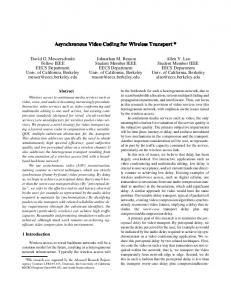
2.1 Physiology of the Human Eye The human eye and its various components are depicted in Fig. 2.1. It contains a transparent liquid, termed vitreous, through which light propagates. The cornea and the lens both focus incoming light onto the retina. The aperture through which light can enter the eye is regulated by the iris. The retina is a thin layer of neural tissue composed of photoreceptors. A portion of the retina, called the fovea, has special properties that will be explained later. It corresponds to the most sensitive area of the eye. The response from the photoreceptors are conveyed to the next stages of vision by the optic nerve. Cornea Lens Iris

Vitreous

Retina Optic nerve Fovea

Figure 2.1: Cross section of the human eye Linear-systems methods can be used to describe the optical transformations performed by the eye as it obeys the principle of linearity [45]. If p1 and p2 are two dierent stimuli and f(p) is the response of the

2.2. PHOTORECEPTORS

11

eye to the stimulus p, the light re ection from the eye obeys the equation: f (p1 + p2 ) = f (p1) + f (p2) ; where  and are two scalar constants. One often de nes the response of the eye to two particular light sources, a line and a point as a function of the aperture of these sources. The respective responses are termed the linespread function and the pointspread function of the eye. The shape of the human linespread and pointspread functions are respectively illustrated in Fig. 2.2 and 2.3. It is known that, as the pupil size increases, the width of these functions increases as well (focus worsens as the pupil size gets larger). 1 0.9 0.8 1

0.7 Relative intensity

Relative intensity

0.8

0.6 0.5 0.4

0.6 0.4 0.2

0.3 0 20

0.2

15

10

0.1 0 −6

10

0

5 0

−10

−4

−2

0 2 Visual angle (arc mins)

4

6

Figure 2.2: Illustration of the human linespread function as a function of the visual angle.

Visual angle (arc mins)

−5 −20

−10 −15

Visual angle (arc mins)

Figure 2.3: Illustration of the human pointspread function as a function of the visual angle.

A very important consequence of the physiology of the human eye is the chromatic aberration. Incoming light is a compound of various wavelengths and both the linespread and pointspread functions vary with the wavelength. Focus will thus vary with the wavelength as well. The consequence is that chromatic fringe will appear around the edges of objects, as each component of the incoming light is focused more or less sharply. The abberation can be seen from the modulation transfer function of the eye as illustrated in Fig. 2.4. The modulation transfer function is represented at a series of wavelengths. The ripples that appear at low wavelengths are the illustration of the chromatic aberration and the change of the modulation transfer with the wavelength. The eye is in focus at 580 nm and this is the wavelength for which resolution is best. At wavelength that are far from the best focus, very poor spatial resolution is obtained. The eye can change its wavelength of best focus by accommodation but it is not possible to focus at all wavelengths simultaneously.

2.2 Photoreceptors The retina is a neural tissue composed of a spatial arrangement of photoreceptors, denoted the photoreceptor mosaic. They convert light information into signals that are interpreted by the nervous system.

12

CHAPTER 2. THE HUMAN VISUAL SYSTEM

1

Sensitivity

0.8 0.6 0.4 0.2 0 0 700

10 600 20

500 30

Spatial frequency (cpd)

400 Wavelength (nm)

Figure 2.4: The modulation transfer function of a model eye, showing chromatic abberation. Their physical characteristics determine their performance in resolution, response time, etc. Consequently they are the source of many limitations of vision.

2.2.1 Types of Photoreceptors There are two dierent types of photoreceptors: the rods and the cones. Rods are much more numerous than cones: there are about 100 millions rods and 5 millions cones per eye and both types are unequally distributed on the retina. Figure 2.5 represents the approximate distribution of cones and rods as a function of the angle relatively to the fovea for the left eye. It can be seen that the majority of cones are concentrated on a very small area that corresponds to the focus of interest, the fovea. No rods are present here. Outside of the fovea, the concentration of cones quickly drops and the concentration of rods increases. There is an area, termed the blind spot, that contains no receptors and that corresponds to the connection of the retina with the optic nerve. Rods initiate vision at low illumination levels. These are called scotopic light levels. They are responsible for vision in the dark and vision of very dim sources. They are small and realize thus a ne sampling of the retina, however many rods are connected to a single neuron for detection. Consequences are that detection is reinforced but visual acuity under scotopic condition is poor. Cones are responsible for vision under photopic conditions, i.e. high light levels. Within the fovea, each cone is connected to several neurons that encode the information. The fovea, that only contains cones, is the area of highest visual acuity. It also corresponds to a null visual angle and thus to the focus of attention of an observer.

2.2. PHOTORECEPTORS

13

# of receptors (mm 2 x 105 )

Rods Cones

1.0

-60

-40

-20

0

20

40

60

Angle relative to fovea

Figure 2.5: Distribution of the cones and rods photoreceptors as a function of the angle from the fovea.

Cones are subdivided into three dierent types according to their wavelength sensitivity. They are termed

L-cones, M-cones and S-cones as they respectively are sensitive to long, medium and short wavelengths.

Figure 2.6 shows the relative sensitivity of the dierent types of cones as a function of the wavelength. A large overlap between L and M-cones sensitivity curves exists. This overlap gives a better spatial resolution (as those wavelengths are sampled nely) and has a strong in uence on the way colors are perceived. It will be seen later that this redundancy between signals from L and M-cones is further decorrelated. The various types of cones have dierent spatial distributions. S-cones are rare in the retina compared to the other two classes of cones and no S-cones are contained in the central fovea. The spatial mosaic of S-cones has been experimentally measured [149] and it has been inferred that S-cones sensitivity is extremely low in the central fovea. Outside of the fovea, the concentration of S-cones is much higher and is distributed according to peaks. It is assumed that those peaks are areas of S-cones separated by large patches of L and M-cones around the fovea. The small concentration of S-cones implies a lower visual acuity at the corresponding wavelength and this is consistent with the strong blurring that occurs due to axial chromatic aberration at lower wavelengths. The spacing between S-cones is about 8 to 12 minutes of visual angle. The L and M-cones mosaic spacing has been estimated experimentally by visual interferometry techniques [148]. Such measurements, along with others [13], give evidence of a sampling frequency of about 60 cpd in the central fovea. The sampling frequency decreases as the distance from the fovea increases. This result is consistent with a change in the granularity of the L and M-cones mosaic. The grid is ner in the fovea and coarser outside of it. It seems that the spacing between two cones in the fovea is about 30 seconds of visual angle. The coarser sampling in L and M-cones outside of the fovea is due to the apparition of rods and the increasing diameter of the cones themselves. It is also to be noted that, outside of the fovea, the cones grid becomes irregular as well.

14

CHAPTER 2. THE HUMAN VISUAL SYSTEM

1 0.9 L−cones

0.8 Normalized sensitivity

M−cones S−cones

0.7 0.6 0.5 0.4 0.3 0.2 0.1 0

400

450

500

550 600 Wavelength (nm)

650

700

Figure 2.6: Spectral sensitivity of the three types of cones as a function of the wavelength. Solid line: L-cones, dashed line: M-cones and dot-dashed line: S-cones.

2.3 Retinal Representation The retina belongs to the central nervous system and is the only part of it that can be easily observed without surgery. There are several classes of retinal neurons and it has been shown by measurements that separate classes of retinal neurons correspond to separate visual pathways. Two classes or retinal neurons are particularly important as they constitute a large fraction of the whole population. These classes are termed parasol and midget ganglion cells. They dier in their morphology. Studies of the connections of retinal neurons with the rest of the nervous system showed that the information transits by the lateral geniculate nucleus (LGN), a structure of the thalamus. Most of the retinal neurons connect to the LGN. The distribution of parasol and midget cells within the LGN is highly regular and is structured in six dierent layers. These are classi ed as parvocellular layers (four super cial layers) and magnocellular layers (two internal layers) according to the dimension of the cell bodies. The structures that can be observed from the retinal ganglion cells to the LGN suggest that there are separate visual pathways. Among those are the parvocellular pathway (beginning with the midget ganglion cells and ending with the parvocellular layers) and the magnocellular pathway (beginning with the parasol cells and ending with the magnocellular layers). The properties of the two pathways have been studied on monkeys [86]. It has been inferred from the study that damages in the magnocellular layers make the animal less sensitive to rapidly ickering low spatial frequency stimuli. Lesions in the parvocellular pathways cause a drop in sensitivity, mostly in spatial frequency at low temporal frequencies. It has also been noted that a loss of information in the

2.3. RETINAL REPRESENTATION

15

magnocellular pathway can be somewhat compensated by the parvocellular pathway.

2.3.1 Cell Response to Light Important properties of visual neurons have been discovered by measuring their electrical response. This is the eld of electrophysiology. In this domain, the concept of receptive eld has been de ned. The visual receptive eld of a neuron is the retinal area in which light in uences the neuron's response. A very important property of the receptive eld is the center-surround organization. In a small central region, light may excite or inhibit a neuron. In a surrounding annular region, the eect of light is opposite. In-between both regions, there is a small area that has mixed response. This is illustrated in Fig. 2.7. The center-surround organization is a key factor and has much in uence on modeling. The property of having an equilibrium between excitatory and inhibitory behaviors will be modeled as such at various stages of this work. Off-response Mixed response On-response

Figure 2.7: Illustration of the center-surround organization of visual neuron.

2.3.2 Contrast Sensitivity Functions A very convenient way of working in a linear-systems kind of formalism is to characterize the considered system's response with respect to a set of harmonic functions. This is also done for the considered description of the visual system and leads to the concept of contrast sensitivity function. The concepts of contrast, contrast threshold and contrast sensitivity have to be developed rst. Contrast is a key concept in vision science. The reason is that the information that is represented in the visual system is not the absolute light level but the contrast, which is the ratio of the local intensity and the average image intensity. Most authors de ne contrast for sinusoidal gratings as: Lmin ; C = LLmax ? max + Lmin where C is the contrast and Lmin and Lmax respectively are the minimum and maximum luminance values. In this work, a de nition of contrast extended to non-stationary random signals is used. This is described in App. A.

16

CHAPTER 2. THE HUMAN VISUAL SYSTEM

Neurons only respond to stimuli above a certain contrast. The necessary contrast to provoke a response from the neurons is de ned as the contrast threshold. The inverse of the contrast threshold is the contrast sensitivity. In this work, it is considered that the contrast threshold for a given stimulus is the contrast value such that the probability of detection of that stimulus is equal to 0:5. Contrast sensitivity varies with frequency, which leads to the concept of the contrast sensitivity function (CSF). It has always been well known that the eye is much more sensitive to lower spatial frequencies than to high ones. The property has been widely exploited to design television sets, cameras or video recorders. The CSF represents the neurons' contrast threshold as a function of the harmonic function. As it will be explained later in the text, the CSF is actually a multivariate function of the spatial frequency, the temporal frequency, the orientation and the color direction. A typical spatial CSF is illustrated in Fig. 2.8 after data from [19].

0

Sensitivity (dB)

10

−1

10

−2

10

0

10 Spatial frequency (cycles/degree)

1

10

Figure 2.8: Illustration of the sensitivity of the human eye as a function of spatial frequency.

An illustration of contrast sensitivity is presented in Fig. 2.9. In this example, both images have been corrupted with white noise ltered by a Gabor lter. The energy of the noise is the same for both images. They thus have the exact same peak signal-to-noise ratio (PSNR). The peak frequency of the lter is however dierent for each image. The image on the left-hand side contains noise around 4 cpd (at a viewing distance of about 6 inches) and the image on the right-hand side is corrupted by noise centered around 16 cpd. The subjective perception of both images is very dierent.

2.4. CORTICAL REPRESENTATION

17

Figure 2.9: Illustration of contrast sensitivity. Both images have the exact same amount of noise with dierent spatial frequency characteristics.

2.4 Cortical Representation The cortex is the cerebral bark of the brain. It is a layer of neurons that is about 2 mm thick. The primary visual cortex, also termed area V1, is located in the occipital lobe of the human brain (posterior area). It receives the connections from the retina and the LGN. Area V1, as the rest of the cortex, has a layered structure. Six layers can be identi ed according to neurons density and connections with the rest of the brain. The pathway topology to area V1 is well de ned and is responsible for some of its properties. The pathway conserves information about:

 the eye of origin,  the ganglion cell classi cation (i.e. the visual stream),  the spatial position of the ganglion cells within the retina. Receptive elds in the visual cortex are very dierent from the receptive elds in the LGN. Their shape is usually non-circular. The most extensive work of physiological study of the primary cortex neurons' response has been made by Hubel and Wiesel [53, 54, 55, 56]. They performed a classi cation of the cortical neurons on the basis of their response to a set of stimuli. They identi ed two categories of neurons, denoted simple cells and complex cells. They dier in the sense that simple cells satisfy the principle of superposition, whereas complex cells do not. A major dierence in behavior between simple and complex cells is in their response to sinusoidal gratings. Simple cells have a response that has the same frequency as the input stimulus (half-wave recti ed), whereas the complex cells exhibit a full-wave recti cation, doubling the frequency of the input stimulus. The receptive eld of simple cortical cells consists of adjacent excitatory and inhibitory areas that make them orientation-selective, as the receptive eld is neither circular nor symmetric. Complex cells also exhibit orientation selective properties. Some specialized neurons are direction-selective. Those neurons

18

CHAPTER 2. THE HUMAN VISUAL SYSTEM

are rare in numbers and are only contained in some layers of the cortex (see Chap. 10). It has also been shown that some of the neurons in the primary cortex are binocular, i.e. they receive input from both eyes. The cortex is the rst stage in the visual pathway that presents binocular properties. As far as visual streams are concerned, area V1 presents an increase in complexity of the visual streams. The two main streams { the parvocellular and magnocellular pathways { reach area V1. The magnocellular pathways splits in two branches. One of the branches connects to an area that is very important in motion perception, the medial temporal (MT). This is consistent with the fact that the magnocellular pathway is more sensitive to higher temporal frequencies. The other branch merges with the parvocellular pathway. This convergence occurs at the level of single neurons receiving input from both pathways. Several new visual streams then begin in area V1. This is however out of the scope of this discussion.

2.5 Pattern Sensitivity Vision science heavily relies on detection and discrimination tests and many models, including the ones proposed in this dissertation, are based on such experiments. The reason is that in most applications, the model will have to predict either if two images or sequences look alike or how easily they can be discriminated one from the other. The study of pattern sensitivity started with Schade [105]. His single-resolution theory models the output of the neurons' receptive eld by a convolution of the data with a convolution kernel. This permits to assess sensitivity of complex patterns just by knowing (and measuring) the sensitivity of a limited set of harmonic patterns. The harmonic functions that Schade considered were sinusoids that he used to measure a spatial CSF. His theory could however not predict sensitivity data accurately. For example, pattern adaptation is a phenomenon that Schade's theory cannot explain. Pattern adaptation denotes the modi cation of the perception of a stimulus due to the adaptation of the eye to another one. Examples of this are thin lines that appears to be bigger and vice versa. This phenomenon is among the evidence of the multi-resolution nature of vision. The single-resolution theory of Schade extended to a multi-resolution formalism is more adapted to predict the desired data. In the multi-resolution theory, the neural representation of an image, the neural image, is a set of images expressed at various scales and sensitive to narrow bands in frequency and orientation. The study of Campbell and Robson [14] gave further proof of the multi-resolution theory. They used square waves and their spectral representation to identify the various mechanisms in human vision. They also highlighted the phenomena of masking and facilitation. Masking occurs when a stimulus that is visible on its own cannot be perceived due to the presence of another one. Facilitation occurs when a stimulus that is not visible on its own permits to discriminate between a stimulus and the addition of the two signals. Figure 2.10 illustrates masking and facilitation. The top left image in the gure is the masker and the top right is the signal to be detected. The signal is clearly visible by itself, as its contrast is above its own threshold. The two bottom images have been generated as follows: the bottom left image is the sum of the masker and the signal, while the bottom right image is the sum of the masker and the signal

2.6. COLOR PERCEPTION

19

rotated clockwise by an angle of 90 degrees. At rst sight the top and bottom left images look alike, as the masker has masked most of the signal. If one looks closely, one can barely see that the images dier slightly, especially on a vertical central line. The top bottom image however looks very dierent from the masker and the signal. As the two signals are no longer closely coupled (they have dierent orientation), the signal is not masked by the masker.

Figure 2.10: Illustration of the masking phenomenon. The top left image is the masker and the top right the signal. The bottom left image has been obtained by summing up the signal and the masker. The bottom right image is the sum of the masker and a rotated version of the signal.

2.6 Color Perception The understanding of color perception depends on the way light is encoded by the brain as a function of its spectral distribution. A brief overview is presented now. The discussion is restricted to photopic wavelength encoding as only photopic vision is relevant to the applications that are addressed. Wavelength encoding can be studied by the color matching experiment. The experiment is meant to study color appearance and is performed as follows: a subject is presented a bipartite screen. Half of the screen is illuminated by a test light, the other half by a mixture of three primary lights. The subject is asked to adjust the primary light so as to match the test light. The experiment shows that human observers have a poor color-discriminability. Lights having very dierent spectral distributions are sometimes perceived as being identical. Such lights are termed metamers.

20

CHAPTER 2. THE HUMAN VISUAL SYSTEM

The color matching experiment can be described using the linear-systems formalism. Let t be a test light that is known by N samples of its spectral distribution expressed as a function of the wavelength. The coecient of the primary light mixture can be found from t and the spectral distribution of the primary lights according to Eq. (2.1):

0 e1 1 0 Color-matching function of Primary 1 1 @ e2 A = @ Color-matching function of Primary 2 A e3

Color-matching function of Primary 3

0 BB B@

t1 t2 .. . tN

1 CC CA ;

(2.1)

where e1 , e2 and e3 are the coecient of the color mixture, the ti 's, with i belonging to the interval [1::N] are the samples of the test light's spectral distribution. The spectral distributions of the primary lights are known and are termed the color-matching functions. They consist of n samples of the spectral distribution of the primary lights. Such a formalism can be used, as it has been proven that a test light can be indeed expressed as the linear combination of the color-matching functions. This is known as the Grassmann's additivity law. Further studies proved that it is possible to completely parameterize the color space with three colors, provided they are linearly independent. The color space is thus a vectorial space of dimension 3. The color-matching functions are not unique, but it is possible to switch from one set of color-matching functions to another by a change of basis. The photopic color matching experiment can also be explained in terms of the light absorption of the cones. To express this in the above formalism, the test light is expressed in terms of the spectral sensitivity of the cones photopigments. This yields Eq. (2.2):

0 0 L 1 0 Spectral Sensitivity of L Photopigments 1 B @ M A = @ Spectral Sensitivity of M Photopigments A BB @ S

Spectral Sensitivity of S Photopigments

t1 t2 .. . tN

1 CC CA ;

(2.2)

where L, M and S represent the respective cone absorptions. However, cones' absolute light absorption cannot explain color perception [132]. For example, a patch of some well-de ned color will look dierent as it lies on a light or dark background. The patch however re ects the same absolute amount of light. Vision scientists quickly suspected that color perception is dependent on the relative cone absorption rates. Hence, the color-matching experiment cannot yield enough data to build a model of color perception. The critical phenomenon that should be explained is the fact that objects look the same under dierent illumination conditions. It is possible [132] to explain such a behavior as a linear transformation of the cones absorption. The linear transformation involved is found by psychophysics. This has been done in the asymmetric color-matching experiment. Basically, the principle of the experiment is identical to the color-matching experiment, the dierence being in the fact that test lights are presented onto dierent backgrounds. The most important results of such studies have been modeled by the so-called opponent-colors theory. The latter, con rmed by experiments, states that some pairs of hues can coexist in a single color sensation while others cannot. For example, the combination of red and yellow is perceived as orange and the

2.7. SUMMARY

21

combination of blue and green is perceived as cyan. On the contrary, a combination of red and green is perceived as two dierent colors. Schematically, it is believed that the brain uses three dierent pathways to encode the information, one conveying the luminance signal, another the red and green components and the third one the blue and yellow components. The opponent-colors theory has been con rmed by the hue cancelation experiment where subjects were asked to set color matches by adding and subtracting opponent colors [61, 57]. Opponent-colors are a way to decorrelate information and their characteristics may be related to the spectral overlap between the sensitivity curves of the L, M and S-cones. The opponent-colors space is thus the appropriate space to work in. A decorrelation of the information between the color components strongly simpli es a model since no inter-component masking phenomenon has to be considered. Mathematically, the transformation to the opponent-colors space is just a linear transformation of the cone absorption and can be cascaded to Eq. (2.2):

0 O1 1 0 L 1 @ O2 A = T @ M A ; O3

S

(2.3)

where O1, O2 and O3 are the weights in the opponent-colors space, and T is the transformation matrix to the opponent-colors space. Recently, Wandell and Poirson have measured color appearance using an asymmetric color-matching experiment to study how color appearance changes with spatial frequency. They derived from this an opponent-colors model [97]. The space that they derived has a particularity that is extremely interesting: it is pattern-color separable. This means that there is no in uence on spatial perception in function of color. The spectral sensitivities of the pathways of that space are illustrated in Fig. 2.11 The existence of the opponent signals is a physiological reality. De Valois et al. [32] showed that there exist opponent-colors neurons in the LGN of non-human primates. The mechanisms that are involved at this level are most probably related to the excitatory-inhibitory nature of the receptive elds. Consider for example a neuron on the red-green pathway; it will be excited by red lights and inhibited by green lights. That neuron will be insensitive to lights that are neither red nor green.

2.7 Summary Many concepts of vision have been presented. They will now be used to build a tractable model of human vision that can be used in a video coding framework. The major concepts that have to be emphasized are the following:

 The neurons that are involved in vision are separated in dierent pathways or streams.  The representation of the information by the visual pathways is the contrast and not the absolute light level.

 Contrast information is represented at dierent scales and orientations.

22

CHAPTER 2. THE HUMAN VISUAL SYSTEM

1 B/W

0.8

R/G B/Y

0.6

Sensitivity

0.4

0.2

0

−0.2

−0.4

−0.6 350

400

450

500

550 600 Wavelength (nm)

650

700

750

Figure 2.11: Spectral sensitivity of the Wandell-Poirson pattern-separable opponent-colors space. The solid line is the luminance channel (termed B/W), the dashed line is the red-green channel (termed R/G) and the dot-dashed line is the blue-yellow channel (termed B/Y).

 Contrast sensitivity of a stimulus varies with the frequency, orientation and the context into which

the stimulus is.  Color representation is highly correlated at the level of the retina and decorrelated into opponent signals in the cortical representation.

Linear systems can be used to describe most of the processing that is done from the lens of the eye to the representation in the primary visual cortex. This approach is used in this work as the objective is to build models that are able to predict the response from the cells in the primary visual cortex to video signals. The prediction is then used for discrimination and identi cation purposes.

Chapter 3

State of the Art in Vision Modeling This chapter reviews some existing vision models. It goes from very basic single-resolution models in Sec. 3.1 to multi-channel models in Sec. 3.2. Each new model corresponds to an increase in complexity. Single-channel models were able to predict simple behaviors of the human visual system but failed in many other cases. The extension to multi-channel models permits the prediction of visibility of more complex patterns. Intra and inter-channel masking then account for more complex phenomena. A brief discussion of this as well as of future research direction is included in Sec. 3.3. Most of the existing models are spatial models. They only predict the visibility of spatial patterns. Although temporal perception and motion perception have been studied, no complete spatio-temporal models have been built so far. The present work is a rst attempt in this direction and will be the subject of the following chapters.

3.1 Single-Channel Models 3.1.1 Schade's Model The rst computational model of vision has been designed by Otto Schade [105] in 1956. His goal was to predict pattern sensitivity for foveal vision. He assumes that the neural image, i.e. the cortical representation of an image, can be obtained by a shift-invariant transformation of the retinal image. The consequence of this assumption is that the shift-invariant transformation can be obtained by determining the response from a single linear receptive eld. The linear receptive eld becomes then equivalent to the convolution kernel of the transformation. Assume that N samples of a one dimensional stimulus x[i] (0  i < N) are known. The neural representation y[i] of the stimulus is obtained as: y[i] =

NX ?1 l=0

h[i ? l]x[l] ;

23

24

CHAPTER 3. STATE OF THE ART IN VISION MODELING

where h[:] is the impulse response of the linear receptive eld. The above equation can be rewritten in matrix notation as Eq. (3.1): 0 h[0] h[?1]


h[?N + 1] 1 0 x[0] 1 0 y[0] 1 BB x[1] CC B B h[1] h[0]


h[?N + 2] C y[1] C C C B B = C C B B .. .. ... A B@ ... CA @ ... @ ... A . . x[N ? 1] h[N ? 1]


h[1] h[0] y[N ? 1]

y = Hx ; where the matrix H is toeplitz [64].

(3.1) (3.2)

The goal is then to have an estimate of H. To do so, Schade measured a set of harmonic contrast patterns. He asked observers to judge the visibility of sinusoidal patterns of varying contrast. These measurements de ne a contrast sensitivity function. Knowing the CSF permits the computation of the convolution kernel by solving for H in Eq. (3.1). The signal h[:], estimated from such measurements, is an estimate of the linespread function and is termed the psychophysical linespread function. In his experiments, Schade suggested that the psychophysical linespread function could be described by the dierence of two Gaussian functions. Schade's model was able to predict quite correctly the visibility of simple patterns. However, the model kept failing as the complexity of the input signal increased. It was not capable of predicting adequately the visibility of mixtures of signals and signals of very low spatial frequencies.

3.1.2 Mannos and Sakrison's Image Fidelity Criterion Another single-channel model came much later and received a large audience in the signal processing community as it was one of the rst works in engineering that used vision science concepts. In their famous paper [80], Mannos and Sakrison recognized that simple computational distortion measure based on the mean squared dierence between two images cannot predict the dierence or perceived quality of one image with respect to the other. On the basis of psychophysical experiments on the visibility of gratings, they inferred some properties of the human visual system and incorporated them in a distortion measure. The experiment they used led them to build an analytical form of the spatial contrast sensitivity function that they later tted to the data. The close-form expression of their CSF, that will be later used in this work, is given in Eq. (3.3):  f  ? fs
c SS (fs ) = d a + f s e? fs0 ; (3.3) s0 where Ss is the spatial sensitivity, fs the spatial frequency and a, d, c and fs0 are parameters to be estimated. They chose a group of subjects and asked them to rate the quality of distorted images. Based on the data of such this test, they estimated the parameters of the CSF and nally obtained the function: SS (fs ) = 2:6 (0:0192 + 0:114fs) e?(0:114fs)1:1 :

3.1. SINGLE-CHANNEL MODELS

25

The distortion measure that they propose consists of multiplying the error spectrum by the CSF and computing its energy. Let I(x; y) be an original image, I^(x; y) be a distorted version of the precedent, and x, y be the spatial coordinates, the Mannos and Sakrison distortion measure e is given by Eq. (3.1.2): e=

Z Z fs 

h i2 SS (fs ) I(fs ; ) ? I^(fs ; ) ;

where fs and  respectively are the spatial frequency and phase values and I(fs ; ) and I^(fs ; ) are the spectra of the original and distorted images. The distortion metric proposed by Mannos and Sakrison is fairly simple as it incorporates few aspects of human vision and is based on the simplest vision model, the single-channel model. It was however the rst work in engineering that linked the elds of image processing and vision science. They proposed the rst comprehensive metric based on physiological and psychophysical evidences of vision.

3.1.3 Other Works Based on Single Channel Models After Mannos and Sakrison's contribution, several other works using a single-channel model of vision appeared in the engineering community. In the major case, the addressed application was image quality assessment or image coding. Some of these works are brie y reviewed below. Nill proposed a weighted cosine transform for the coding of digital images [91]. His model is an extension of the model by Mannos and Sakrison. Its innovation is the adaptation of the formulation of the contrast sensitivity function to the use of the discrete cosine transform (DCT) representation of the data so as to have a tractable model that can be incorporated in DCT-based coders. A follow-up of Mannos and Sakrison's work and Nill's work has been carried out by Saghri et al. [103]. They combined both contributions and further re ned the model to better account for display device calibration, viewing distance and image resolution. There is however no signi cant improvement of the visual model compared to the one proposed by Mannos and Sakrison. Lukas and Budrikis [77] were the rst to propose a model for moving pictures. They developed a tool that assesses the quality of television images for digital picture coding applications. Their distortion measure is based on a spatio-temporal model of the contrast sensitivity function. The CSF, that lters the error signal, is modeled as the division of an excitatory and inhibitory path, each path being linear. Masking is then incorporated in their model as a weighting of the ltered error based on the activity of the original picture. The nal stage of the metric, the summation rule for the masked error signal, is done over blocks of the image chosen so that a block has the dimension of the foveal eld. This is the rst vision model that can be used for video applications. It has interesting features, such as the non-linear modeling of the CSF and the use of visual masking. However, it is limited in the sense that it will fail where every single-channel model fails. Moreover, new developments about the spatio-temporal CSF are now known [11] and provide a better modeling of it.

26

CHAPTER 3. STATE OF THE ART IN VISION MODELING

3.2 Multi-Channel Models Single-channel models fail to predict pattern visibility in many cases. They are not able to cope with patterns of very low spatial frequency, complex patterns or mixtures of patterns. Moreover, psychophysical studies [14] gave evidence of the multi-resolution structure of visual perception. Vision scientists moved to multi-channel models and some of them are discussed here.

3.2.1 Watson's Works Andrew B. Watson has been a very active and productive vision scientist. His works addressed many aspects of human vision and he proposed several models with his group. An interesting tool introduced by Watson is the cortex transform [139]. It is a decomposition tool that simulates the various mechanisms of vision. The decomposition is somewhat similar to the Laplacian pyramid [12]. The lters are bandpass in spatial frequency and orientation and have an approximate Gabor shape. Four orientations are considered as well as four spatial frequency bands. The spatial lters follow an octave band partitioning of the frequency axis. At each frequency level, the data are subsampled but not critically subsampled, i.e. there will be no aliasing in the subbands as it occurs with the wavelet transform [101]. The transform is invertible by simple upsampling and addition. The ltering operation is implemented as a multiplication operation in the frequency domain. The cortex transform has then been used as the decomposition tool for many of Watson's work. A complete spatial vision model for image coding has been introduced in [138]. The cortex transform is used there as a rst analysis stage of the data. Pattern sensitivity is then modeled with a contrast sensitivity function and intra-channel masking. The ltered signals are then quantized by a perceptual quantizer that minimizes the perceived error. The cortex transform has also been used in a discriminability model [5] to predict object detection on natural backgrounds. The multi-channel model is compared with a simple single-channel model. The multi-channel model only considers intra-channel masking. The conclusion of the study was that, for that particular application, both models performed equally well. The HOP transform has been introduced as an alternative decomposition tool [144]. The HOP transform is a hexagonal orthogonal-oriented quadrature pyramid which operates on a hexagonal input lattice. It uses basis functions that are orthogonal, self similar and jointly localized in space, phase, frequency and orientation. There are seven basis functions (one low-pass and six band-pass). The transform has a pyramidal structure and eachplevel is computed from the previous level. Levels are subsampled so that the spacing at each level is 7 larger than the previous one. The downsampling factor is 7 between two levels. The transform is a complete representation of the input image and approximates correctly frequency and orientation bandwidth of the cortical neurons. The representation however suers some drawbacks: the lters have a secondary lobe in the direction orthogonal to the main lobe. The high downsampling factor (7) yields fewer scales than necessary and the rotation invariance of the transform is reduced. Finally the channels of the HOP transform are broader in orientation than in frequency while cortical cells realize the opposite.

3.2. MULTI-CHANNEL MODELS

27

A very well known tool developed by Watson is the so-called DCTune algorithm [141, 142]. It is an algorithm designed to optimize the quantization matrices of the JPEG coding standard [44]. The algorithm is image-dependent and minimizes the perceptual coding noise. The optimized quantization matrix accounts for visual masking by luminance and contrast techniques and by an error pooling over all blocks of the image. Watson has been the rst to outline the architecture of a vision model for sequence processing [140]. The model is a straightforward extension of the spatial model that he previously introduced (e.g. [138]). However, the model has not been implemented.

3.2.2 The Visible Dierences Predictor (VDP) A well-known vision model is Scott Daly's. He proposes an algorithm for determining image delity as a function of the display parameters and viewing conditions. The output of his model is a map indicating the areas in which two images dier in a perceptual sense. His vision model is made of three parts: an amplitude non-linearity, a contrast sensitivity function and a hierarchy of detection mechanisms. The amplitude non-linearity accounts for the light adaptation of the retina to the environment. It describes the changes that occur due to dierent illuminations conditions. It basically ensures that very dark and very bright areas will not be over or under estimated. The CSF that he uses is anisotropic and is slightly dierent from the Mannos and Sakrison formulation. The general shapes of the curve are however pretty similar. The frequency hierarchy detection is implemented as follows: consider two images, an original and a distorted one. Both images, which have been rescaled by the nonlinearity and the CSF, are decomposed by a lterbank into several channels. The decomposition tool is Watson's cortex transform. A masking function, that is close to a non-linear transducer described in Chap. 4 is then used to weight the dierence image. The masked perceptual components of the dierence image is then multiplied by a psychometric function that describes the increase in detection probability as the contrast increases. Finally, probability summation is used to pool the data over the various channel and combine them into a single image that predicts the visibility of artifacts.

3.2.3 A Model for Image Coding Applications Serge Comes's work [19] proposes a spatial vision model for image coding applications. The vision model in itself has many similarities with Watson's. Several decomposition tools can be used in his model to implement the channel decomposition. Some applications use a classical Gabor bank. A perfect reconstruction lter bank is introduced for restoration applications. The bank is close to the Gabor bank, has no subsampling operation and oers invertibility. Finally, a non-separable lterbank can be used, especially for coding applications. Several aspects are worth noting in this work. First of all the model has been especially designed for image coding applications and has been parameterized by psychophysical experiments with these constraints in mind. Several interesting applications are investigated in this model, namely image restoration, for

28

CHAPTER 3. STATE OF THE ART IN VISION MODELING

which several schemes are considered, taking advantage of the perceptual decomposition [78, 21].

3.2.4 Foley and Boynton's Model Legge and Foley [71] proposed a theory of simultaneous visual masking that sums excitation linearly over a receptive eld. This results in a model that only considers intra-channel masking. Neurophysiological experiments carried out on the cat [10] demonstrated however that there exists a broadband interaction in pattern vision. The studies showed that the cortical cells receive a broadband divisive input besides the linear summation over the receptive eld. Heeger then proposed a model of the cat cortical cell responses where the cell response is modeled by the division of an excitatory mechanism (the linear sum over the receptive eld) divided by a broadband inhibitory mechanism [49, 50]. Foley and Boynton [40] carried out experiments on simultaneous masking of Gabor patterns by sinewave gratings. In these experiments, target contrast thresholds were measured as a function of the masker contrast, orientation, spatial phase and temporal frequency. They used such results to test the Legge and Foley theory. A very important result of their study is the eect of masker orientation on the threshold curves. A conclusion is that there exists some inter-channel masking and that this phenomenon can be signi cant. An illustration of the types of measurement that they obtained is given in Fig. 3.1 and 3.2. Consider two stimuli, a masker and a target. Let CT 0 denote the detection threshold of the target measured in the absence of a masker (i.e. given by the CSF), CT be the detection threshold of the signal in the presence of a masker and CM be the contrast of the masker. If the masker and the target have the same orientation, the diagram of masking looks like the one depicted in Fig. 3.1. There is a region, when CM < CT 0 , where the masker has no in uence on the perception of the target. When CM > CT 0 , the detection contrast for the target grows exponentially with the contrast of the masker (i.e. detection of the target is harder). When the contrast of the masker and the target are very close one to the other, the curve presents a dipper. This means that, at this value of contrast, the masker actually helps detection of the target (this is known as the facilitation eect). When the target and the masker dier in orientation, the detection curve looks as the one depicted in Fig. 3.2. The dierence with the previous case is that the curve does not present a dipper around CM = CT 0, there is no facilitation eect. Foley and Boynton proposed a model of masking that is derived from Heeger formulation [49, 50] in which the response R of a cortical cell is obtained as the division of an excitatory input E with a summation of all inhibitory inputs Ij given by Eq. (3.4): p (3.4) R = P EI q + z ; j j where p, q and z are constants. In this formulation, the presence of the dipper can be quite simply explained. If the masker and the target have approximately the same orientation, a contribution at that orientation appears both in E and one Ij , decreasing the value of R. On the contrary, when both signals have dierent orientations, there is no simultaneous contribution to E and an Ij .

3.2. MULTI-CHANNEL MODELS

29

log C T

log C T ε

ε

C T0

C T0 log C M

log C M

C T0

C T0

Figure 3.1: Detection contrast curve for a target in the presence of a masker. The masker and the target have approximately the same orientation.

Figure 3.2: Detection contrast curve for a target in the presence of a masker. The masker and the target have dierent orientations.

3.2.5 A Normalization Model On the basis of his modeling of the cat cortical cell's response and the data from Foley and Boynton, Heeger proposed with Teo a delity metric for still pictures [113, 114]. The tool is of interest to this work as it will be extended to the processing of video sequences. The model is based on the following building blocks:

   

a front end linear transform, squaring, normalization, detection.

The linear transform stage decomposes the image into perceptual channels. It is implemented with hexagonally sampled quadrature mirror lters or cosine lters in [113] or the steerable pyramid [107] from Simoncelli et al. in [114]. The coecients at the output of the linear transform are squared and normalized. Since the output coecients of the transform linearly increase with the input magnitude, it is desirable to restrict the output to a certain dynamic range (as it is the case in an actual system like the cortex). Let A be a coecient of the output of the linear transform having orientation . The normalized output for the coecient, R , is computed by Eq. (3.5): R = k P

?A
2

 (A )

2 + 2 ;

(3.5)

where  ranges over all orientations, k is a global scaling constant and  a saturation constant. Pooling is only performed across orientation and not across spatial frequency as inter-channel masking is restrained

30

CHAPTER 3. STATE OF THE ART IN VISION MODELING

to channels having the same frequency [40]. The values for constants k and  have been obtained by tting the model to Foley and Boynton's data. Finally, a detection mechanisms predicts how dierent two images may look. Assume that Ro is a vector gathering all the sensors output computed by Eq. (3.5) for an original image and Rd be the equivalent vector for a distorted version of the considered image. The distortion measure is computed as squared error norm of the dierence between Ro and Rd using Eq. (3.6):
R = jRo ? Rd j2 :

(3.6)

3.3 Comments Some studies investigated the performance of various types of model. Among those is the study by du Buf [34]. Some of his conclusions are that single-channel models predict quite correctly the visibility of very simple signals (sinewave gratings) of medium frequency. They usually fail at low spatial frequencies and cannot predict the visibility of non-sinusoidal gratings or mixtures of signals. Simple multi-channel models provide good prediction of threshold curves of sinewave gratings and other gratings. They however fail for more complex signals such as disk-shaped stimuli. The use of global or local probability summation within channels can predict the shape of the threshold curves for disk-shaped signals or noise gratings but the sensitivity values are under-estimated. Possible improvements of such models could be obtained by a local probability summation across channels or by a combination of isotropic channels (at the retina level) followed by anisotropic channels (at the cortex level).

Chapter 4

Spatio-Temporal Vision Modeling Chapter 2 pointed out the most relevant facts about vision that a model should account for. Those characteristics are the existence of several visual streams, the adaptation to the environment and the multiresolution representation of the information. The various streams are dierent pathways throughout the entire visual system that are each responsible for the analysis and interpretation of the retinal image. The visual system is able to adapt itself to the various conditions into which it has to operate (as compensation for high variation of illumination level). A consequence of this characteristic is the use of relative contrast to represent the visual information instead of the absolute light level. Finally, the most salient characteristic of vision is the multiresolution representation of the data into which contrast information is represented at various scales, in precise orientation and frequency bands. In chapter 3, some models of human vision have been presented. They all restricted themselves to spatial vision. The early models where single-resolution models (also termed single-channel models). They only account for the global contrast sensitivity characteristics of vision. Further models incorporated the multi-resolution aspects. More recent and advanced models now incorporate modeling of further aspects as inter-channel masking. This chapter introduces the modeling of spatio-temporal vision that this work proposes. Here is shown how components of the visual system are described. The description starts with the modeling of the vision mechanisms in Sec. 4.1. The important issue of non-separability between spatial and temporal perception is then addressed in Sec. 4.2. Section 4.3 reviews contrast sensitivity and masking is presented in Sec. 4.4. The general architecture of the model is described in Sec. 4.5 and Sec. 4.6 summarizes the chapter.

4.1 Mechanisms of Human Vision The responses of the receptive elds in the cortex have shown to be band-selective. This behavior is modeled as a multiresolution representation of the data in the cortex. Perception is thus thought to be mediated by a collection of individual mechanisms, denoted channels, that are each selective in orientation, 31

32

CHAPTER 4. SPATIO-TEMPORAL VISION MODELING

spatial frequency and temporal frequency. Psychophysical experiments can be used to determine the nature of such mechanisms. The study of perception of narrow-band signals close to threshold is used to determine the number and width of the channels. As the combination of all channels has to yield the global contrast sensitivity, a measure of the CSF completes such study. In this way, an estimation of the number, shape and position of mechanisms involved in vision is known.

4.1.1 Spatial Mechanisms The cortical receptive elds have a pro le that is very similar to Gabor function[28, 100] and some authors [104, 66] associate this to an optimal encoding that would be performed by the brain (since Gabor patches are the functions that are the most compact both in spatial or temporal and frequency domains). Psychophysical experiments measured the bandwidth of spatial vision mechanisms. It has been found that the frequency bandwidth is around one octave and the orientation bandwidth between 20 and 40 degrees. An important result has been evidenced by De Valois et al. : they showed [31] that the frequency and orientation bandwidth of the spatial channels are correlated. The dependence has been studied by Daugman [27], who came up with the relationship described in Eq. (4.1):

 2
! ? 1  ;
 = arcsin  2
! + 1

(4.1)

where
 is the orientation bandwidth of the mechanism,
! is the frequency bandwidth and  is an aspect ratio between 0:5 and 1. Byram measured [13] that the sampling frequency of the cones mosaic is around 60 cpd. Summing theses considerations together, the spatial frequency plane is thought to be covered by about 5 frequency-selective mechanisms and 4 to 9 orientation mechanisms.

4.1.2 Temporal Mechanisms Temporal mechanisms have been studied too. There is however less certainty about their number and shape than for temporal lters. Early studies [92, 72] concluded that there is a large number of mechanisms narrowly tuned. This result has now been contradicted and most authors refer to the existence of two or three temporal lters. Watson and Robson found out [133] that human beings are only able to discriminate between low and high temporal frequencies. This result, con rmed by other studies, also has physiological evidence. Foster et al. [41] showed that cortical neurons of the macaque are tuned for temporal frequency and may be either band-pass or low-pass. However, some authors [79, 51] argued for the existence of a third, high frequency temporal channel. The mechanism is thought to only exist at low spatial frequency (below 0:5 cpd). A key evidence for the existence of the third temporal mechanism is the improvement in discrimination at high temporal frequencies (above 30 Hz). The study of Hammett and Smith [48] reevaluated the question. They showed that the improvement is not real but is an artifact of the dierence in the rate of perceptual fading as

4.2. SPATIO-TEMPORAL INTERACTIONS

33

a function of temporal frequency. It is indeed known that when a ickering stimulus is viewed for a prolonged time, the perceived icker gradually fades. This work thus assumes the existence of only two temporal mechanisms, denoted transient and sustained mechanisms. The sustained mechanism is low-pass and the transient one is bandpass with a peak frequency around 8 Hz. Parameters of the lters are taken from the study of Hess and Snowden [52].

4.2 Spatio-Temporal Interactions A model of human vision has to use the contrast sensitivity function as a key building block. A close form formula of it is thus necessary. The proposed model needs a spatio-temporal CSF. The easiest formulation that one would use is a separable model, that is a model where the spatio-temporal sensitivity could just be expressed as the product of spatial and temporal sensitivity. In this case, the CSF would be written as: S(fs ; ft) = SS (fs ) ST (ft ) ; where fs and ft are the spatial and temporal frequencies, S(fs ; ft ) describes the spatio-temporal CSF, SS (fs ) and ST (ft ) respectively are the spatial and temporal sensitivity functions. Many studies pointed out that this formulation is wrong and that there is a strong interaction between spatial and temporal perception. This is easily seen if one measures the temporal sensitivity at various spatial frequencies. The curves do not change by just a scale factor but their shapes change with spatial frequency. It is known that sensitivity is higher in regions of low spatial and high temporal frequencies as well as in regions of high spatial and low temporal frequencies.

4.2.1 Excitatory-Inhibitory Formulation Burbeck and Kelly [11] gave an excitatory-inhibitory formulation of the spatio-temporal threshold surface based on the hypothesis that the surface can be expressed as the dierence between the responses of two separable mechanisms. Each mechanism is low-pass both in temporal and spatial frequency. The rst mechanism accounts for the peak sensitivities and the cuto, while the second mechanism decreases the response in the low temporal and low spatial frequency region. The denomination excitatory-inhibitory model comes from the antagonism of the mechanisms. More concretely, the modeling is the following: as the mechanisms are assumed to be separable, the spatial and temporal response curves of the inhibitory mechanism are set to be the dierence between the excitatory mechanisms and the measured surface respectively at low temporal frequency and low spatial frequency. The spatio-temporal surface is then the product of the spatial and temporal response curves. This is mathematically expressed as follows: let E(fs ; ft) represent the excitatory mechanism and I(fs ; ft ) be the inhibitory mechanism. The mechanisms are written as: (4.2) E(fs ; ft ) = K1 SS;ft1 (fs ) ST;fs1 (ft )

? ? (4.3) I(fs ; ft ) = K2 E(fs ; ft2 ) ? SS;ft2 (fs ) E(fs2 ; ft) ? ST;fs2 (ft ) ;

34

CHAPTER 4. SPATIO-TEMPORAL VISION MODELING

where the spatial frequencies fs1 and fs2 and the temporal frequencies ft1 and ft2 are chosen to measure the temporal sensitivity curves ST;fs1 (ft ) and ST;fs2 (ft ) and the spatial sensitivity curves SS;ft1 (fs ) and SS;ft2 (fs ). Eventually, the spatio-temporal sensitivity function is expressed as in Eq. (4.4) by taking the dierence of the excitatory and the inhibitory mechanisms: S(fs ; ft ) = E(fs ; ft ) ? I(fs ; ft ):

(4.4)

The excitatory-inhibitory formulation relies on physiological grounds. It is indeed intimately related to the excitatory-inhibitory characteristics of the receptive elds' response in the LGN and the cortex [132]. The spatio-temporal response of neurons in the parvocellular layers of the LGN of the macaque have been measured [33]. The measurements showed the dependence highlighted here above. The data showed a decreased sensitivity at low spatial frequencies (due to the strong opponent surround of the receptive elds). The neurons exhibited a strong response at all temporal frequencies when a low spatial frequency was used. The response strongly decreased at high temporal frequency when high spatial frequencies were used. This showed that the responses from the on-center and the surround of the receptive elds were dierent. It can be however measured that the center and the surround have space-time separable responses. Modeling the CSF by two separable opponent mechanisms, as proposed by Burbeck and Kelly is thus motivated.

4.2.2 Multi-Resolution Modeling of the Spatio-Temporal Interaction Burbeck and Kelly's approach proposes a very tractable and simple model of the spatio-temporal CSF. The formulation is however single-channel and only describes the global CSF. As temporal sensitivity changes with spatial frequency and vice-versa and since sensitivity is dictated by the response of individual mechanisms, it is important to know how this spatio-temporal dependence re ects at the level of the mechanisms themselves. Several schools of thought exist. One explanation is that the temporal lters have a peak sensitivity that is dependent on spatial frequency [67, 150]. This is denoted the sensitivity-scaling hypothesis. Another school of thought assumes that the population of lters exhibits a spatio-temporal covariation. This is the covariation hypothesis. Both hypotheses are depicted in Fig. 4.1. The sensitivity-scaling hypothesis states that a variation of the gains of the lters as a function of their position in the spatio-temporal frequency plane models the phenomenon. In this case, a lterbank separable along the spatial and temporal directions can be used. The covariation hypothesis implies that the position of the peak frequencies changes with the area of the spatio-temporal frequency region. In this case, the lterbank cannot be separable. Hess and Snowden [52] undertook a study of the number of temporal lters, of their individual temporal properties and of their relative peak sensitivities using a masking paradigm. The technique permits the measure of the relative sensitivities of the temporal lters. The conclusion of the study gave evidence for the sensitivity scaling hypothesis, meaning that the covariation in the spatio-temporal threshold surface may be due to a simple variation of the gains of the lters. The number and shape of the temporal mechanisms did not change radically and the sensitivity scaling is sucient to model the threshold surface.

35

Temporal frequency

Temporal frequency

4.3. CONTRAST SENSITIVITY

Spatial frequency

Spatial frequency

Figure 4.1: Illustration of the sensitivity-scaling hypothesis (left hand side) and the covariation hypothesis (right hand side). The ovals represent the bandwidths of the lters in the spatio-temporal frequency plane. In the rst case, the position of the lter along the temporal frequency axis is invariant, which is not the case in the second hypothesis. The existence of two temporal and six spatial mechanisms has been assumed. The result has been assumed in this work. The consequence on the proposed model is that the collection of vision mechanisms is modeled by a lterbank that is separable in spatial and temporal frequencies. The spatio-temporal interaction is then modeled at the level of the respective gains of the lters.

4.3 Contrast Sensitivity Burbeck and Kelly's excitatory-inhibitory formulation of the spatio-temporal CSF is very convenient and tractable. It allows to estimate the CSF on the basis on many less data points than a totally nonseparable formulation. Moreover, data tting is much easier as there are fewer parameters to estimate. A close-form expression of the whole threshold surface can thus be obtained with the expression of the spatial and temporal sensitivity curves. Mathematical models of the latter are now presented.

Spatial Sensitivity Both the physiological and psychophysical studies showed a low-pass behavior of the eye and a high-pass behavior of the retina [29]. The general behavior is band-pass with a peak sensitivity around 2 to 8 cpd and a cuto frequency around 64 cpd. The model of this dependence that is most used has been proposed by Mannos and Sakrison [80], and relates the spatial sensitivity Ss to the spatial frequency fs according to Eq. (4.5):  fs  ? fs
c SS (fs ) = d a + f e? fs0 ; (4.5) s0

where the parameters a, d, c and fs0 have to be estimated. The parameter fs0 is the peak frequency and d is a simple gain constant. The in uence of a and c are less intuitively perceived. The in uence of a is illustrated in Fig. 4.2 where the function SS (fs ) is plotted for three values of a, showing that the parameter accounts for the shape of the curve at low frequencies. Figure 4.3 shows the eect of c on SS (fs ). The parameter sets for the steepness of the slope of the high frequency limb of the curve.

36

CHAPTER 4. SPATIO-TEMPORAL VISION MODELING

0

0

10

−1

10

10

−1

Sensitivity

Sensitivity

10

a = 0.1 −2

−2

10

a = 0.01

10

c = 1.1

a = 0.001

c = 0.95 c = 0.8

−3

10

−3

10

−1

10

0

10 Spatial frequency (cpd)

−1

10

1

10

Figure 4.2: Illustration of the in uence of the parameter a on the spatial sensitivity function.

0

10 Spatial frequency (cpd)

1

10

Figure 4.3: Illustration of the in uence of the parameter c on the spatial sensitivity function.

Temporal Sensitivity An ecient model of temporal sensitivity has been described by Watson [137]. The temporal sensitivity is modeled by the cascade of two linear lters modeling the transient and sustained mechanisms and is: ST (ft ) =  (H1 (ft ) ? H2(ft )) ;

(4.6)

where ft is the temporal frequency, ST (ft ) is the temporal contrast sensitivity function and H1(ft ) and H2(ft ) are the frequency responses of the two linear lters.  is a gain factor and  is the transience factor. A mathematical expression of the frequency response of the two lters in Eq. (4.6) is: H1(ft ) = (2jft  + 1)?n1 H2(ft ) = (2jft  + 1)?n2 :

(4.7)

The parameter  is a time constant, j is the imaginary unity, n1 and n2 account for the steepness of the transition band of the lters and  is the ratio of the time constants of the two lters. The temporal sensitivity function is thus expressed as:





ST (ft ) =  (2jft  + 1)?n1 ?  (2jft  + 1)?n2 : The parameters n1 and n2 account for the steepness of the high-pass limb of the two mechanisms. The gain is controlled by . The time constant  regulates the bandwidth of the curve as Fig. 4.4 illustrates it. Figure 4.5 shows the in uence of the parameter  that is the ratio of the time constants of both mechanisms. The relative in uence of each mechanism is controlled by  that weights the in uence of the transient mechanism with respect to the sustained one as illustrated in Fig. 4.6.

4.4. MASKING

37

2

10

2

Sensitivity

Sensitivity

10

1

10

1

10

tau = 0.002

kappa = 1.0

tau = 0.004

kappa = 1.33

tau = 0.01

kappa = 2.0

0

10

0

10

1

2

10 Temporal frequency (Hz)

10

Figure 4.4: Illustration of the in uence of the time constant  on the temporal sensitivity function.

0

10

0

10

1

10 Temporal frequency (Hz)

2

10

Figure 4.5: Illustration of the in uence of the parameter  on the temporal sensitivity function.

2

Sensitivity

10

1

10

zeta = 1.0 zeta = 0.9 zeta = 0.0

0

10

0

10

1

10 Temporal frequency (Hz)

2

10

Figure 4.6: Illustration of the eect of the parameter  on the temporal sensitivity curves. The parameters weights the contributions of the transient mechanism with respect to the sustained one.

4.4 Masking Masking is a very important phenomenon in vision as it quantizes the interactions between dierent signals. As Legge and Foley de ned it [71], masking refers to \any destructive interaction or interference

38

CHAPTER 4. SPATIO-TEMPORAL VISION MODELING

among transient stimuli that are closely coupled in space or time" Consider two dierent stimuli on the same test image. The presence, and the features of one stimulus will in uence the way the other one is perceived. Both signals will indeed interfere and their relative perception will be modi ed. In actuality, the detection threshold of one stimulus will be modi ed as a function of the contrast of the other. Masking has been intensively studied [70, 71, 108]. It has been shown that its eect is maximal when the stimulus and the masker are closely coupled (in terms of orientation, spatial and temporal frequencies) and decreases rapidly as the distance between the considered signal increases in the spectral domain. Masking is illustrated in Fig. 4.7. Consider two stimuli, the \signal" and the \masker" that are closely coupled. Let CT 0 denote the detection threshold of the signal measured in the absence of a masker, as obtained from the CSF, CT be the detection threshold of the signal in the presence of a masker and CM be the contrast of the masker. The discussion restricts for now the the formulation of Legge and Foley [71]. log C T

log C T

ε ε

C T0

C T0 log C M

log C M C T0

Figure 4.7: Illustration of the masking phenomenon.

C T0

Figure 4.8: Non-linear transducer model of masking.

Three regions can be identi ed [70]:

 At low values of CM , the detection threshold remains constant, that is CT = CT 0.  As CM gets closer to CT 0 , the detection threshold slightly decreases, and presents a dipper. At such

contrast value, the presence of the masker actually helps detection of the signal. This phenomenon has also been termed negative masking, facilitation or the pedestal eect.

 Finally, as CM increases, CT increases as a power of the contrast masker. This function is linear in a log-log graph and its slope is denoted ".

A common model of masking consists of a non linear transducer. It is illustrated in Fig. 4.8. The simpli cation introduced is the absence of a dipper. This model is used in most of the present work. The Legge and Foley study of masking [71] pointed out that the masker and the stimulus to be detected had to be closely coupled so that masking would be eective. If such a consideration is made in a multi-resolution theory, where the vision model is composed of several mechanisms, it would mean that

4.5. GENERAL ARCHITECTURE

39

each mechanisms is independent from the other and that masking can only occur between two stimuli that are located in the same channel. Many vision models are based on such an assumption [26, 20, 19] and only consider intra-channel masking. In a more recent study, Foley and Boynton [40] characterized masking of Gabor patterns by sinewave gratings. They showed that the Legge and Foley theory is inadequate as they could measure a signi cant amount of inter-channel masking. Now, more advanced vision models incorporate inter-channel masking [113, 114, 108, 134]. This work proposes several models. Both approach, i.e. intra-channel only and intra and inter-channel masking, are addressed.

4.5 General Architecture Having described the functional building blocks of the vision model, the general architecture of it can be described. Video applications are the focus of this work and the vision model has to be considered in such a framework. Consider some original video sequence material s and a corrupted version of it sd . The distorted sequence is assumed to be the result of a compression/decompression process by a digital video coder. The corrupted sequence can be expressed as sd = s + e; where e is the coding noise, i.e. the distortion introduced by the compression/decompression process. The latter generally is a complicated signal as it is the combination of many dierent artifacts resulting from the various tools that the video coder uses. The task of the vision model is to assess or estimate the visibility of the signal e. Applications could be quality assessment, coder regulation or image enhancement. This formulation implies that e can be considered as a target stimulus, the visibility of which is being predicted, while s is a masker to e. There will thus be masking of the coding noise by the original sequence. The proposed architecture is depicted in Fig. 4.9. In this case, only a processing of the luminance signal is considered. Original Sequence

Perceptual Decomposition (Linear Transform)

Perceptual Components Weights

Pattern Visibility Decoded Sequence Coding Noise

Perceptual Decomposition (Linear Transform)

x

Pooling

Perceptual Components

Figure 4.9: Architecture for the vision model. This architecture only processes luminance information. The thick arrows represent a set of perceptual components. The thin lines represent video sequences. The signal e is rst computed by subtracting the original sequence from the distorted one. The next stage is a linear transform. Its goal is to emulate the multiresolution structure of vision by predicting the channel decomposition done at the level of the primary visual cortex. This linear transform is a bank of lters that have characteristics similar to the mechanisms of vision. The output of the linear

40

CHAPTER 4. SPATIO-TEMPORAL VISION MODELING

transform is thus a set of signals representing the data at various scales and resolution. Such signals are termed perceptual components. Both the original signal and the coding noise are processed by the linear transform. Pattern visibility is then predicted. Two phenomena are considered at this stage. The rst is contrast sensitivity that permits to predict the visibility of a single patterns, the second is masking that quanti es the relative change in sensitivity due to the presence of a masker signal. The perceptual components of the original sequence and of the coding noise are the input of this building block. Weights are computed and the perceptual components of the coding noise are multiplied by these weights. The weights quantize the visibility of each pixel of the coding noise's perceptual components. They are equal to the sensitivity (i.e. the inverse of the computed detection threshold). This expresses the data relatively to the detection threshold. The data is the set to be expressed in units above threshold or just noticeable dierences (jnd's). The nal stage gathers all the individual data together. This is the pooling stage. The previous stages give a prediction of the responses from the neurons in area V1 of the cortex. It is believed that higher stages, initiating with area V2, integrate the information represented at various scales and orientations. Pooling simulates this process by integrating the data according to some summation rules. An architecture taking color into account is proposed in Fig. 4.10. It has essentially the same structure as the luminance-only architecture and features all the building blocks of it, namely the linear transform, pattern visibility and pooling. The architecture contains a front-end block that decorrelates color information. Section 2.6 addressed color perception and pointed out that color information is encoded according to three pathways that respectively convey the luminance, red-green and blue-yellow information, which constitute the opponent-colors space. The front end block of the color architecture simulates this phenomenon. It converts the data from the color space into which the sequences are represented to the opponent-colors space. Usually, the working color space for video coding is (Y, U, V) or (Y, Cr, Cb) [89]. It is to be noted that the computation of the coding noise has to be done after the conversion to the opponent-colors space. Next chapter will point out that the conversion is a non-linear process as it has to account for display device calibration. Once the data is represented in the opponent-colors space, each pathway is processed separately, as the information has been decorrelated. Each pathway undergoes the linear transformation and the pattern visibility prediction. Separate data for detection threshold have to be known, as perception varies with color. Kelly showed [65] that the spatio-temporal CSF of the chromatic channels can be modeled using the excitatory-inhibitory formulation as well. Eventually, the pooling stage gathers all the information together according to a summation rule across frequency, orientation and color directions.

4.6 Summary This chapter presented the proposed spatio-temporal vision modeling. The various building blocks that are needed to construct the model have been presented. It has been pointed out that the multi-resolution structure of the cortex has to be predicted by simulating the detection mechanisms of vision. The number and characteristics of such mechanisms have been described. The important issue of spatiotemporal separability has then been addressed and it has been shown at which stage of the model the non-separability can be modeled. This resulted in an expression of the spatio-temporal sensitivity function

Original Sequence

Y, Cr, Cb to BW, RG, BY

Decoded Sequence

4.6. SUMMARY

Y, Cr, Cb to BW, RG, BY

41

Perceptual Decomposition (Linear Transform)

BW RG BY

Perceptual Components Weights

Pattern Visibility BW RG BY

Perceptual Decomposition (Linear Transform)

Coding Noise

x

Pooling

Perceptual Components

Figure 4.10: Architecture for the color vision model. The thick arrows represent a set of perceptual components. The thin lines represent sequences. that is used in the prediction of pattern sensitivity. The other phenomenon onto which relies pattern sensitivity is masking. A model of masking has been described. Finally the general architecture of the vision model has been presented. Two architectures are proposed, one processing only the luminance information and the other including color perception.

Chapter 5

Implementation of the Vision Models The general architecture of the vision model has been presented in the previous chapter. This chapter now discusses several solutions to implement it. Each solution corresponds to an increase in modeling complexity. The basic model, presented in Sec. 5.1 incorporates the most important characteristics of vision, that is to say multiresolution architecture and modeling of pattern sensitivity. A variation of this model is then proposed in Sec. 5.2 for speci c applications requiring perfect reconstruction of the data. Section 5.3 describes the third model that adds processing of color. The fourth model is the subject of Sec. 5.4. It goes back to the sole processing of luminance but addresses two limitations of the previous models, one being the computational complexity involved and the other being the modeling of the cortical receptive elds responses. Sec.5.5 then summarizes the previous developments.

5.1 Basic Spatio-Temporal Vision Model The goal of this model is to incorporate the fundamental tools that are needed to model spatio-temporal vision. As it is - to our knowledge - the rst spatio-temporal multi-channel model for video applications, it is meant to investigate the possible bene ts that a vision model could bring to video sequence processing. As it has been seen that multiresolution is one of the key aspects and that signi cant bene ts can be obtained by modeling the vision mechanisms. This rst model is not single-resolution and models the channels that partition the frequency domain. The other phenomena that are modeled are contrast sensitivity and masking. This model has been described in [119].

5.1.1 Gabor-Based Perceptual Decomposition As the pro le of the responses of the cortical neurons has a Gabor shape, the lters used to emulate the cortical mechanisms are Gabor lters. This choice has the advantage of yielding a representation 42

5.1. BASIC SPATIO-TEMPORAL VISION MODEL

43

that should be close to the cortical representation. The disadvantage of Gabor lters is that they are very selective in the spectral domain and thus have a large extend in the pixel domain. The ltering operation has then to be performed in the frequency domain. This means that a Fourier transform of three-dimensional data has to be computed. The computational load is high and a large delay is involved [128]. The lters used in the model are analytical, similarly to Comes' decomposition. This means that the lters are only de ned for positive frequencies. As the input signal is real-valued, the output of the ltering operation, which is a complex signal, has a real part that is equal to the result of the ltering by a symmetric lter. The advantage of analytical lters is that the contrast of the signal can be computed as the magnitude of the complex ltered signal as described in App. A.

Spatial Filters The spatial lters have to be selective in orientation and radial frequency. They are separable along those dimensions in a polar coordinate system. Another characteristic of the spatial mechanisms is that they realize an octave-band partitioning of the frequency axis. The lters are then generated according to Eq. (5.1) that de nes the lters' frequency response as a function of the spatial frequency f and the orientation  for a lter that is centered at a frequency of f0 , an orientation of 0 and that respectively has a spatial and orientation bandwidth of
f and
:

? log2(f=f0 )
2 ?? ?0
2

Gf0 ;0 (f; ) = e?


f

e




:

(5.1)

The low-pass lter is dierent. At very low spatial frequency, the concept of orientation does not make much sense, hence the lter is isotropic. The DC component is not of interest for many applications. The objective of the model is to predict detection of artifacts or discrimination between an original sequence and a corrupted one. A change in the global luminance level has no importance as the eye is sensitive to the relative luminance level. Therefore, the low-pass lter does not include the DC component. Its frequency response is given by Eq. (5.2): 2

G(f) = e(
fa ) ? e f

? f
2
fb

;

(5.2)

where
fa = 2 cpd and
fb = 0:25 cpd. Based on the consideration of Sec. 4.1, a number of ve frequency bands are used (including the low-pass isotropic lter) and four orientations. This makes up a total of seventeen spatial lters. The lterbank is illustrated in Fig. 5.1, where the frequency response of the lters is plotted onto the spatial frequency domain between ?32 and +32 cpd.

Temporal Filters Two mechanisms are considered for temporal vision. The rst one corresponds to the sustained channel that is sensitive to lower temporal frequencies. This channel is modeled by a low-pass lter, the frequency response of which quickly drops around 4 Hz. The second mechanism is represented by a band-pass lter

44

CHAPTER 5. IMPLEMENTATION OF THE VISION MODELS

32

Frequency (cpd)

16

0

−16

−32 −32

−16

0 Frequency (cpd)

16

32

Figure 5.1: The spatial lter bank featuring 17 lters (5 spatial frequencies and 4 orientations). The magnitude of the frequency response of the lters is plot on the frequency plane. The lowest frequency lter is isotropic. that has a peak frequency around 8 Hz. The lters are Gabor lters as well and are designed in the spectral domain. The parameters from those lters are taken from [52]. The resulting lterbank is illustrated in Fig. 5.2

5.1.2 Contrast Sensitivity The lterbank is separable in temporal and spatial frequency. As pointed in Sec. 4.2 of the text, the spatiotemporal interaction that vision exhibits is modeled at the level of the contrast sensitivity function. The CSF is non-separable in spatial and temporal frequencies and follows the excitatory-inhibitory formulation of Burbeck and Kelly [11]. The exact parameters of the surface have to be determined by psychophysics. This process is described in Chap. 6. The exact surface that has been used is described in that chapter.

5.1.3 Masking The description of visual masking by Legge [70] is assumed for this model. It is considered that masking occurs when two stimuli are closely coupled in the spectral domain. They must have similar orientation, spatial frequency and temporal frequency, i.e. a stimulus can only mask another if both of them belong to the same channel. This is the hypothesis of independent channels.

5.1. BASIC SPATIO-TEMPORAL VISION MODEL

45

0

Magnitude

10

−1

10

0

1

10

10 Temporal frequency (Hz)

Figure 5.2: The temporal lter bank accounting for two mechanisms: one low-pass (the sustained mechanism) and one band-pass (the transient mechanism). The frequency response of the lters is presented as a function of temporal frequency. The model for masking is the non-linear transducer depicted in Fig. 5.3. It assumes that the detection threshold remains constant up to the point that the contrast of the masker reaches the value of the detection threshold. The detection threshold then grows monotonically with the masker contrast in an exponential way. This model neglects the facilitation eect that occurs when the masker contrast is close to the detection threshold (see Sec. 4.4). log C T

ε

C T0 log C M C T0

Figure 5.3: Non linear transducer model of masking. The detection threshold CT for a stimulus can then be computed as a function of the detection threshold

46

CHAPTER 5. IMPLEMENTATION OF THE VISION MODELS

of that stimulus in the absence of a masker, CT0 (i.e. as given by the contrast sensitivity function) and the contrast of the masker CM . The relationship is given by Eq. (5.3): CT =

(C

T 0  " CT 0 CCTM0

if CM < CT 0 if CM  CT 0 :

(5.3)

5.2 Perfect Reconstruction Perceptual Decomposition The Gabor lterbank used in the previous model does not oer perfect reconstruction which is sometimes desired. Some applications may require perfect reconstruction of the data once they have been processed in the channels. A few works proposed Gabor expansion that oers perfect reconstruction properties [152]. Such an approach is not used here. The position and number of lters that should be used is quite rigid and ideally, a decomposition that is close to the one performed in the previous model is desired. Therefore, the solution that is chosen is to design a lterbank that exhibits perfect reconstruction properties and is more similar to the Gabor lterbank. Van Calster and van der Plancke [116] designed with Serge Comes such a decomposition for still pictures. The design procedure of the lterbank can be summarized as so: the perfect reconstruction lterbank (PR bank) should be very similar to the Gabor bank in terms of number and bandwidth of lters. As the ltering operation can be performed in the spectral domain, the lters are designed in frequency. Perfect reconstruction is required, but the decomposition does not entail any decimation of the data. This greatly reduces the complexity of the lter design procedure. Let Gf0 ;0 (f; ) be a lter centered at frequency f0 and orientation 0 , expressed in function of the radial frequency f and orientation . The lter is chosen to be polar-separable and is described by Eq. (5.4): Gf0 ;0 (f; ) = Hf0 (log(f)):H0 () ;

(5.4)

where H(:) is the frequency response of a lter. The constraints that are needed to obtain perfect reconstruction can be met by specifying that H(:) is a continuous function and satis es the constraints in Eq. (5.5): H(x) = 0 in the stop-band, H(x) = 1 in the pass-band, H(xs ? x) + H(?xs ? x) = 1 in the transition band,

(5.5)

where x is the variable and xs is a value in the transition band of the lter. The perfect reconstruction constraint is met when the value of xs is the same for two adjacent lters. Van Calster and van der Plancke chose Eq. (5.6) as the function for the transition band of the lters:

 8 1  < 2 1 ? sin 2 sign(x ? xs) x?xsxs  if 0  x  2xs; x+xs   H(x) = : 1  1 + sin sign(x + x ) if ? 2xs  x < 0: s xs 2 2

(5.6)

5.3. A COLOR MODEL

47

The parameter  has a value between 0 and 1 and accounts for the steepness of the transition band. A lterbank has been built using the above prototypes for lters. The bank features twenty-one lters. The rst seventeen lters have the same frequency and orientation tuning as the lters of the Gabor bank. The last four lters are included for reconstruction purposes. They have a peak frequency of 32 cpd, to complete the coverage of the frequency axis and are tuned to the four chosen orientations. The magnitude of the frequency response of the bank is depicted along the frequency axis in Fig. 5.4 along with the Gabor bank. The dashed line represents the PR bank and the solid line the Gabor bank. Both banks realize similar frequency decompositions. 1

Magnitude

0.8

0.6

0.4

0.2

0 0

5

10

15 20 Spatial Frequency (cpd)

25

30

Figure 5.4: Comparison of the Gabor and PR spatial frequency decomposition. The dashed line is the PR bank. The solid line is the Gabor bank. The magnitude of the frequency response of the lters is plotted versus spatial frequency. A temporal lterbank has been designed using the same procedure to have a spatio-temporal PR decomposition. The bank features three lters. The rst two lters account for the sustained and transient mechanisms of temporal perception. They have approximately the same peak frequency and bandwidth as the Gabor lters depicted in Fig. 5.2. The last lter covers the higher frequency region and ensures that the sum of the frequency responses equals unity. The bank is shown in Fig. 5.5.

5.3 A Color Model The color architecture proposed in this work is a direct extension of any of the two previous models. As it has been pointed out earlier, a perceptual processing of color data is most eciently done by working in an appropriate color space, namely the opponent-colors space. The opponent-colors space decorrelates color

48

CHAPTER 5. IMPLEMENTATION OF THE VISION MODELS

1

Magnitude

0.8

0.6

0.4

0.2

0

0

1

10

10 Spatial Frequency (cpd)

Figure 5.5: Comparison of the Gabor and PR temporal frequency decomposition. The dashed line is the PR bank. The solid line is the Gabor bank. The magnitude of the frequency response of the lters is plotted versus temporal frequency.

Original Sequence

information as it approximates the representation of the data in the various visual streams of the visual system. Each of those streams are independent, hence a separable processing of each color component can be done. The architecture is illustrated in Fig. 5.6. Two new building blocks appear. They are the linearization block and the conversion to opponent-colors. Perceptual Components

B/W

Linear Color Space

Opponent-Colors Space

Perceptual Decomposition

R/G B/Y

Weights

Decoded Sequence

Masking B/W

Linear Color Space

Opponent-Colors Space

R/G B/Y

-

Distortion Measure

Perceptual Decomposition

Coding Noise

x

Pooling

Perceptual Components

Figure 5.6: Implementation of the color model.

5.3.1 Linearization of the Data The digital samples that are known from the video sequence are termed the frame-buer values. Those samples are expressed in some color space (usually (Y, U, V) or (Y, Cr, Cb) in video coding). However those values are not linear with the luminance as produced by the display device. The device performs some gamma correction and the luminance of the screen also depends on the phosphor of the screen itself. The rst step is to transform the data into a calibrated space to be device-independent and to be

5.4. SPATIO-TEMPORAL NORMALIZATION MODEL

49

able to apply further color space transformation. The exact procedure for display device calibration is explained in App. B. The output of this non-linear block is a compound of three streams that are now in a device-independent space and are linear with luminance.

5.3.2 Conversion to Opponent-Colors Space The next step converts the data to the opponent-colors space. The transformation chosen in this work has been designed by Wandell and Poirson [97, 98, 131, 132]. This transformation oers the additional advantage of being pattern-color separable. This particular opponent-colors space will be further referred to as the Wandell-Poirson space (WPS). As explained earlier, the conversion to the opponent-colors space is a simple linear transform. The transformation matrix is given in App. C. The output of this module are three streams that are the color components in the opponent-colors space. The three pathways are termed luminance (B/W), red-green (R/G) and blue-yellow (B/Y). The B/W component is extremely close to the luminance channel of the (Y, U, V) or (Y, Cr, Cb) spaces [89].

5.3.3 Number of Color Channels Human sensitivity to color chrominance component is much lower than to luminance information. This is a direct consequence of the characteristics of the photoreceptors mosaic in the retina, namely the spacing of the various types of cones. This feature has been extensively used in engineering, where the chrominance information is usually downsampled with respect to the luminance information. It follows that a restrained number of channels can be used for the R/G and B/Y pathways. Along the temporal direction, only the sustained mechanism is to be considered as temporal sensitivity drops very quickly for chrominance. In the spatial domain, the rst three frequency bands are used, as sensitivity is very low above 8 cpd. Those considerations are based on the work by Watson [140].

5.4 Spatio-Temporal Normalization Model This model is based on the model by Teo and Heeger described in [113, 114]. As pointed out in Sec. 3.2.5, the normalization model oers several advantages, namely:

 it models the data from Foley and Boynton [40],  it models the normalization of the cortical receptive elds' response,  it accounts for intra and inter-channel masking,  it has a linear transform stage that is carried out in the pixel domain,  it uses a pyramidal decomposition scheme.

50

CHAPTER 5. IMPLEMENTATION OF THE VISION MODELS

The model has been extended to account for spatio-temporal perception. The decomposition has been designed to ensure low delay. The block diagram of the model is presented in Fig. 5.7. The various building blocks are a subband decomposition, an excitatory-inhibitory stage, a normalization procedure and detection. Perceptual Components

Perceptual Decomposition (Linear Transform)

Original Sequence

Inhibitory Mechanism Normalization Excitatory Mechanism Detection

Decoded Sequence

Inhibitory Mechanism

Perceptual Decomposition (Linear Transform)

Normalization Excitatory Mechanism Perceptual Components

Figure 5.7: Block diagram of the normalization model.

5.4.1 Subband Decomposition As in the previous models, the subband decomposition is done separately in time and space. The dierence between this implementation and the others, is that the whole decomposition is carried out in the pixel domain. No Fourier transform is needed, which eliminates the high delay that was induced. Special care has been taken for the temporal decomposition so as to minimize temporal delay of the whole decomposition stage. This implementation can thus be used for applications that require short response time, such as video quality regulation (see Sec. 11.1).

Spatial Decomposition The spatial decomposition is done as in the Teo-Heeger model [114]. It uses the steerable pyramid developed by Simoncelli et al. [107]. The transform decomposes an image into spatial frequency and orientation bands. It is implemented as a recursive pyramidal scheme, an illustration of which is presented in Fig. 5.8. The basis functions have octave bandwidth. The number of bands has been chosen to be equal to the Gabor implementation, i.e. 5 frequency band, one of which (the DC one) being isotropic, and 4 orientation bands. The orientation decomposition is steerable for each frequency band, i.e. it is invariant by rotation. The steerable pyramid oers many advantages compared to other decomposition schemes such as wavelet transforms [101]. In the wavelet transform, the subband signals are critically subsampled which results in aliasing in the subbands. Aliasing is cancelled at the reconstruction stage only, which can be a problem

5.4. SPATIO-TEMPORAL NORMALIZATION MODEL

51

H0

H0

Li-1

B0

B0

B1

B1

B2

B2

B3

B3

Li

2

2

Li-1

Li

next stage of the pyramid

Figure 5.8: Analysis/synthesis representation of the steerable pyramid. H0 is a high-pass lter, the Li 's are low-pass lters and the Bi 's are orientation lters. when processing the subband data1 . Another problem of the wavelet representation is that it is not shift invariant. The steerable pyramid has been designed to obtain a multiresolution representation of an image, decomposing it in frequency and orientation bands that are rotation invariant. The price to pay for this is that the representation is over-complete, expanding the data by a factor of 16=3 [107].

Temporal Decomposition A temporal lter bank is proposed. The main constraint that has been imposed when designing it is low delay. Some applications that would use a perceptual decomposition may require very fast response from the system. Consider for example a buer regulation scheme for an encoder. The quantization parameter have to be adapted as a function of the desired quality and occupancy of the output buer. Such decisions have to be made as quickly as possible. For this reason, no subsampling operation is performed along the temporal direction. This was chosen so as to have as much degrees of freedom as possible in designing the temporal lterbank. The bank also has to approximate the Gabor temporal bank depicted in Fig. 5.2 to a reasonable approximation. Doing so with nite impulse response lters (FIR lters) may require lters having as much as 6 to 8 taps, which is a too long delay. Therefore in nite impulse response (IIR) lters have been chosen to implement the temporal decomposition. A maximum delay of 3 frames has been imposed. Such a delay is reasonable as many implementations of actual coders, namely MPEG coders, have such delays. The lters have been designed by minimizing the dierence between their frequency response and the Gabor lters response in a least square sense. The optimization procedure yielded a low pass lter that has one pole and one zero. This lter approximates the sustained mechanisms. The transient mechanism is approximated by a 3 poles and 2 zeroes lter. Finally, a third lter is designed to yield the high pass residue (so as to have an invertible transform). This lter added to the sum of the two others yields a 1

cross processing between subbands is sometimes necessary as shown by Gilloire and Vetterli [43].

52

CHAPTER 5. IMPLEMENTATION OF THE VISION MODELS

at response. All lters are listed in [75]. The low pass and band pass lters are presented in Fig. 5.9 along with the corresponding Gabor lter.

0

Magnitude

10

−1

10

0

1

10

10 Temporal frequency (Hz)

Figure 5.9: Comparison of the magnitude of the frequency responses of the Gabor temporal bank (solid line) and the proposed IIR lterbank (dashed line).

5.4.2 Excitatory-Inhibitory Stage The excitatory mechanism consists of a local measure of the energy. It consists of a squaring operation of the output of the linear transform stage. Squaring is used to introduce a contrast-dependence on sensitivity and thus weight higher contrasts more that lower ones. The inhibitory mechanism also consists of an energy measure, however it is pooled over the other channels. This is of course related to the excitatory-inhibitory characteristics of the cortical neurons' receptive elds. The inhibitory mechanism is pooled over orientation channels as inhibition is much more broadly tuned than excitation [40].

5.4.3 Normalization The normalization stage consists of the ratio of the excitatory and inhibitory mechanisms. Normalization preserves the essential features of linearity but is restricted to a limited dynamic range. Let A be a coecient of the output of the linear transform having orientation . The normalized output, R , of the

5.5. SUMMARY

53

coecient A is computed by Eq. (5.7):

?


A 2 mechanism response = k R = k Excitatory P (A)2 + 2 ; Inhibitory mechanism response 

(5.7)

where  ranges over all orientations, k is a global scaling constant and  a saturation constant. Pooling is only performed across orientation and not across temporal and spatial frequency as inter-channel masking is restrained to channels having the same frequency [40]. The values for the constants k and  have to be found for each band. The values have been obtained by simulating a target at threshold contrast. For this stimuli, the sum of the output of all sensors should equal unity. The contrast sensitivity function experimentally obtained in Chap. 6 has been used for this purpose.

5.4.4 Detection The nal detection stage is a simple squared-error norm [113, 114]. Let Ro be a vector collecting the sensor outputs for the original image sequence and Rd be the vector of sensor outputs for the distorted sequence. The detection mechanism computes the vector distance
R using Eq. (5.8):
R = jRo ? Rd j2 :

(5.8)


R then is a prediction of the visibility of the dierence between the two sequences.

5.5 Summary Four implementations of the spatio-temporal vision modeling have been presented. Each implementation has its application and corresponds to an increase in complexity compared to the previous ones. The rst model is a \vanilla" implementation. It accounts for the very basic properties of human vision, namely the multiresolution structure of the cortical representation and pattern sensitivity. Pattern sensitivity accounts for contrast sensitivity, models the spatio-temporal interaction of the receptive elds and intra-channel masking. The objective of the model is to validate the perceptual approach for video processing. The second model is very similar to the previous one. The linear transform block is changed to a perfect reconstruction transform. The model can be used for applications requiring reconstruction of the data. The third model adds processing of color. It is built on top of the previous models and accounts for color perception by a projection of the data onto an opponent-colors space. The color space used has the property to be color-pattern separable, hence each color component can be processed independently. Eventually, the fourth model is a very dierent implementation. The objective of this model is to account for further concepts of vision such as inter-channel masking and non-linear summation properties of the receptive elds. It is an extension of the Teo-Heeger normalization model.

Chapter 6

Parameterization of the Model The models, as described in Chap. 4 need to be parameterized. An estimate of the contrast sensitivity function is needed. As this work focuses on speci c signals, namely coding artifacts, the estimation of the CSF is done with respect to a model of such signals. The estimation of such parameters belongs to the eld of cognitive psychology and more precisely to psychophysics. Section 6.1 describes the setup of the experiments that have been carried out. The description of the experiments themselves is performed in Sec. 6.2 and the result of the experiments are given in Sec. 6.3 and Sec. 6.4 concludes this chapter.

6.1 Psychophysical Experiments Psychophysics is the eld that designs reliable methods for the study of sensory processes. Psychophysical experiments study the behavior of the human visual system modeled as a black box. This is done by designing an experiment into which human observers (the \subjects") are presented stimuli that they have to detect. On the basis of the subjects' answers and of a theoretical model of the experiment, parameters of the human visual system are evaluated. Two types of psychophysical tests exist: explicit and implicit measurements. In the rst case, a group of subjects is shown pictures or sequences and subjectively judge their quality. In the second case, the subjects are presented standard, synthetic waveforms and objective parameters are estimated. The latter are further divided into several types of experiment among which [37, 19]:

 Method of limits: The contrast of a target stimulus is increased step by step, then decreased step

by step. The estimated contrast threshold is the mean of the results obtained by increasing and decreasing the contrasts. The method is very easy and fast but inaccurate.

 Method of adjustment: The contrast of the target stimulus is adjusted by successive approximations, oscillating around the detection threshold. As the previous one, the method is fast but inaccurate. 54

6.1. PSYCHOPHYSICAL EXPERIMENTS

55

 Method of constant stimuli: is used to obtain more accurate estimates of thresholds. The principle is based on a psychometric function that models the experiment (e.g. the percentage of correct answers of the subject for a given stimulus). The experiment consists then in estimating several points of the psychometric function.

One of the most robust and most used constant stimuli test is the N -alternatives forced choice. In this test, every presentation of a stimulus is made in a sequence divided into N subsequences. The stimulus is present in one and only one of the subsequence and the task of the subject is to give a position for the subsequence containing the stimulus. An N-alternatives forced choice can be modeled by the logistic curve [111, 46]:   N ? 1 1 ; (6.1) P(C) = N 1 + 1 + e ?(xS?M ) where P(C) is the probability of correct answers at the testing level x. M is referred to as the midpoint and S as the spread of the psychometric function. A probability of 0:5 means that the subject does not perceive anything (and gives purely random answers). The threshold of detection (de ned as a detection probability of 0:5) is characterized by a probability of correct answers of 0:75. M and S are the parameters that can be estimated from the experiment. An ecient way to do so is to use a so-called PEST (parameter estimation by sequential testing) procedure [111, 112]. It is a scheme that sequentially chooses the testing level and makes decisions on whether to stay at that level or to change to another. An initial testing level is chosen (well above the threshold to be estimated) and the number of correct and incorrect answers of the subject are counted, yielding an estimation of the probability of perceiving the stimulus. As soon as the estimated probability gets out of a con dence interval centered at 0:75, a new level is chosen adaptively as is the step to proceed to the future level. The estimation of the parameters M and S has been further improved by Hall [46], who performs a maximum likelihood estimation of the parameters of the psychometric function given the measured data. An a posteriori con dence test can be further added [47] to decide on the quality of the measurement.

6.1.1 Example of an experiment An example of a test is now described. The nature of the stimuli will be de ned later. The present subsection is intended to illustrate the N-alternatives forced choice experiment and the PEST procedure. The experiment has been performed on subject RC. A rough estimation of the detection threshold for the kind of stimulus considered had been obtained and gave a value around M0 = ?4 dB. The minimum step size to adjust levels has been chosen to be S0 = 0:5 dB. The procedure was a two alternatives forced choice (2AFC) and 44 sequences have been presented to subject RC. The test started at a level of M0 + 4 S0 , which is ?2 dB. The stimuli levels and answers as a function of the sequence number are presented in Fig. 6.1. Whenever the ratio of correct answers to number of trials got out of the con dence interval, a new stimulus level and step size were chosen according to the PEST rules [111]. After the maximum number of allowed sequences, the test was stopped to avoid tiredness of the subject. The parameters of the psychometric function are then estimated by maximum likelihood estimation [46, 85]. The result is depicted in Fig. 6.2. The nal results gave an estimated threshold of about ?5:16 dB.

56

CHAPTER 6. PARAMETERIZATION OF THE MODEL

Data for subject RC, Jun 13 17:30:44 1995 −1.5 −2 −2.5

Stimulus level (dB)

−3 −3.5 −4 −4.5 −5 −5.5 −6 −6.5 0

5

10

15

20

25

30

35

40

45

Run

Figure 6.1: Graph of the stimuli threshold and subject's answer as a function of the presented sequences. A cross represents a correct answer and a circle an incorrect one. The adaptation of the step can be clearly seen.

6.2 Description of the Experiment 6.2.1 Subjects Five subjects took part in the experiments. They will hereafter be referred to by their initials as IB, LP, RC, SF and BD. The group consisted of four men and one woman. Four of the subjects are working in the eld of image processing and the fth one is not. They were all optically corrected if they needed it.

6.2.2 Apparatus A Sony monitor model BVM-2010P has been used for the experiment. It has been calibrated and was connected to a real time display device controlled by a computer. The control software chose the level of the stimuli and displayed the corresponding sequences. The subjects were seated at a distance equal to six times the height of the screen and the experiment was conducted in a semi-darkened room. One experiment was conducted per day for each subject.

6.2. DESCRIPTION OF THE EXPERIMENT

57

Data for subject RC, Jun 13 17:30:44 1995 1 0.95 0.9 0.85

Probability

0.8 0.75 M = −5.162971

0.7

S = 0.4470979 0.65 0.6 0.55 0.5 −10

−9

−8

−7

−6 −5 −4 Stimulus level (dB)

−3

−2

−1

0

Figure 6.2: Maximum likelihood estimation of the parameters of the psychometric function. The data is plot as a function of the stimulus level. The psychometric curve is then tted to the data.

6.2.3 Method The method used was a two alternatives forced choice (2AFC). The level of the stimuli was controlled by a PEST procedure [111, 112]. The estimation of the parameters was done by maximum likelihood estimation [46]. Whenever a data set had been collected, an a posteriori con dence test [47] was run to decide whether to keep the data set or discard it. Thresholds were measured as the 75% point on the psychometric curve described in Eq. (6.1). No more than 45 sequences are presented to the subject per experiment to avoid eye tiredness and decrease of concentration.

6.2.4 Stimuli The purpose of the work is to characterize the perception of coding artifacts, therefore, the stimuli used are not sine waves or square waves as it is usually the case. In an analogous manner to Serge Comes' work [19], the stimuli used are Gabor patches. The choice is motivated by the fact that such a signal is close to the decomposition of coding noise by a perceptual channel. If sinewave gratings were used, the predicted contrast sensitivity would have been too low to predict the visibility of coding noise [34]. The signal that has been used here is white noise ltered by a tri-dimensional Gabor function tuned in spatial frequency, orientation and temporal frequency. The lters have been normalized so that the integral of the squared frequency response is unity.

58

CHAPTER 6. PARAMETERIZATION OF THE MODEL

The temporal evolution of the sequences shown to a subject is illustrated in Fig. 6.3 and is built as follows: a picture made up of a dark background onto which a circle of medium luminance is surimposed is shown to the subject. This is the \pause interval". Then follows a testing interval, followed by the pause interval followed by another testing interval followed by a nal pause interval. A stimulus appears in only one of the two testing intervals. The testing intervals have been signaled to the subject by four little grey patches located in the corners of the screen. The subject gives an answer after the second testing interval. The answer has to be the position of the interval during which the subject thinks the stimulus was present. Probability of stimulus presence

0.5

pause interval

test interval

pause interval

test interval

pause interval

Figure 6.3: Illustration of the 2AFC procedure. Every sequence presented to a subject is decomposed into pauses and testing intervals. There are two testing intervals by sequence and only one contains the stimulus. The sequence is illustrated in Fig. 6.4. The frame dimension is 256256 pixels. The background luminance is the minimum luminance according to CCIR Rec. 601 [17]. The circle has a radius of 100 pixels and a luminance of 128. The border of the circle is smoothed out onto 15 pixels to prevent Mach eects. When a stimulus is added to a frame, it is tted to a disk, the center of which coincides with the center of the big circle. The circle of the stimulus has a radius of 40 pixels and the borders are smoothed out onto 4 pixels. Eventually, when a stimulus is presented, its magnitude is progressively increased and decreased to avoid a ash eect. The duration of the onset and oset is 40 msec. The total duration of a sequence is 6:48 sec. The testing intervals are each 1 second long.

6.3 Results of the Experiments Characterization of spatio-temporal sensitivity has been performed over a period of four months between March and July 1995. The experiments were stopped when every subject had three correct and complete sets of data. The following assumptions have been made about the contrast sensitivity function. Considering the

6.3. RESULTS OF THE EXPERIMENTS

59

Figure 6.4: Three typical frames of the testing sequences. From left to right: (1) the image indicating a pause interval. The subject knows that no stimulus is present. (2) A testing frame where no stimulus has been inserted. The little square patches in the corner indicate the nature of the frame. (3) A testing frame with a stimulus. excitatory-inhibitory formulation, Eq. (4.4) can be rewritten as:

?

S(fs ; ft) =  SS;ft1 (fs ) ST;fs1 (ft ) + SS;ft2 (fs ) ST;fs2 (ft )+


SS;ft2 (fs ) ST;fs1 (ft ) +  SS;ft1 (fs ) ST;fs2 (ft ) ;

(6.2)

where ; ; and  are normalization factors and where the spatial and temporal curves are respectively described by Eq. (4.5) and Eq. (4.6). The individual gains of those curves have been set to unity since the gain can be controlled by the factors ; ; and . The value of  has been set to the highest measured value, that is  = 2:08. It has been assumed that the two spatial sensitivity curves have the same peak frequency fs0 , which under the light of other studies is quite reasonable [11, 52]. For temporal sensitivity, it has been assumed that the curves would dier by the time constant  and the ratio of time constants .

6.3.1 Characterization of Temporal Sensitivity at a given Spatial Frequency The rst set of experiments characterized temporal sensitivity at a spatial frequency of 4 cpd and an orientation of 45 degrees. Measurements have been made at temporal frequency of 4, 8, 16 and 32 Hz. The measurements for the ve subjects are presented in Fig. 6.5 and are reported in Tbl. 6.1. The sensitivity of the subjects varies but the general shape of the curve is very consistent with the theoretical prediction. It can be clearly seen that the band pass characteristic predicted by the model is obtained in the measurements. As reported in other studies [137, 52, 48], a peak sensitivity is obtained around 8 Hz. The data points have been averaged over the subjects and tted to the model, using Eq. (4.6) as the temporal sensitivity model. The notation of Eq. (4.6) is used here. Common values for n1 and n2

CHAPTER 6. PARAMETERIZATION OF THE MODEL

Sensitivity (dB)

60

0

10

IB RC LP BD SF −1

10

4

8 16 temporal frequency (Hz)

32

Figure 6.5: Graph of the measured sensitivity for the ve subjects as a function of temporal frequency and at a spatial frequency of 4 cpd.

Subject LP IB RC SF BD

Temporal Frequency (Hz) 4 8 16 32 0:4014 0:2838 0:4370 4:2255 0:2172 0:1852 0:2737 1:6113 0:2759 0:2072 0:3481 3:2882 0:5737 0:3813 0:6316 7:2527 0:3956 0:3305 0:4773 4:3857

Table 6.1: Measured data point for the ve subjects at the four tested temporal frequencies. Each data point is the the result of the average of 3 successful measurements.

respectively are 9 and 10 [137] and have been assumed. For convergence purposes,  has been set to 0:8. The result of the data tting process, illustrated in Fig. 6.6, is:  = 0:0052;  = 1:2;  = 7:5:

Sensitivity (dB)

6.3. RESULTS OF THE EXPERIMENTS

61

0

10

0

10

1

10 frequency (Hz)

Figure 6.6: Estimated temporal sensitivity curve at a spatial frequency of 4 cpd based on the psychophysical measurements. The circles indicate the average observed values among the subjects. The solid line represents the t of the model to the data.

6.3.2 Spatio-Temporal Sensitivity The previous measurements, combined with those obtained by Serge Comes [19] and the measurement of two other points of the spatio-temporal curve are used to estimate the spatio-temporal CSF. The additional measurements have been performed at a temporal frequency of 32 Hz and spatial frequencies of 2 and 16 cpd. The complete set of data, including the measurement of Serge Comes after gamma correction is reported in Tbl. 6.2. Spatial Frequency (cpd) and Temporal Frequency (Hz) (2,0) (4,0) (8,0) (16,0) (4,4) (4,8) (4,16) (4,32) (2,32) (16,32) 1:2192 1:5049 0:6263 0:0758 2:8353 3:7370 2:4003 0:2688 1:2098 0:0269 Table 6.2: Measured data point used for the estimation of the spatio-temporal CSF. The data has been tted to the excitatory-inhibitory model described previously by a least square t. The result of the tting process is illustrated in Fig. 6.7 and Fig. 6.8. The data obtained are: = ?0:08;

= 0:081;  = 3:74; c2 = 1:99;

62

CHAPTER 6. PARAMETERIZATION OF THE MODEL

1

10

0

Sensitivity (dB)

10

−1

10

−2

10

−3

10 2 10

0

10

1

10 −2

Temporal frequency (Hz)

10

0

10

Spatial frequency (cpd)

Figure 6.7: Representation of the estimated spatio-temporal CSF. 2 = 0:011; a2 = 37:92; 2 = 1:09:

6.4 Conclusion This chapter presented the psychophysical experiments that have been carried out in order to have an estimate of the human spatio-temporal contrast sensitivity function. A robust testing method in cognitive psychology, namely the N-alternatives forced choice has been used controlled by an adaptive algorithm, the PEST method. Synthetic stimuli, modeling coding noise, have been presented to a group of ve subjects. The resulting data have been used to obtain an estimate of the excitatory-inhibitory formulation of the spatio-temporal CSF as described in Chap. 4. An estimate of the contrast sensitivity to coding noise is thus known and can be used to assess pattern sensitivity and regulate the gains of the lters emulating the channel decomposition.

6.4. CONCLUSION

63

0.5

1 3

2 4.5

4

1

Temporal frequency (Hz)

10

3.5

1.5 2.5

0.5

0

10

1

−1

10

0

1

10

10 Spatial frequency (cpd)

Figure 6.8: Contour plot of the estimated spatio-temporal CSF.

64

CHAPTER 6. PARAMETERIZATION OF THE MODEL

Part II

Applications

65

Chapter 7

On Testing of Digital Video Coders Video transmission systems are currently in a state of transition from a completely analog system to a digital system. Digital video will bring a tremendous amount of new services, possibilities and applications. Besides digital video broadcasting and video on demand (VOD), visual communications and more general multimedia applications will play an important role in tomorrow's everyday life. Digital video source coding has been investigated for years and some coding methodologies have been standardized, the digital system which will be extensively deployed will incorporate source coders employing the MPEG compression standards [1, 3]. From a systems viewpoint, the analog to digital transition is problematic since unlike analog video systems, the methodology to test digital coding systems has not been formalized, neither been much investigated. It is however mandatory to be able to design a methodology for end-to-end testing of digital video delivery systems. The existing approaches are quite recent and focus on testing the MPEG bitstream syntax [84]. An innovative testing methodology is proposed and described in this chapter. A prototype of the proposed testing device, also presented in [123] is introduced. The testing device consists of a test pattern generator (TPG) wherein the test patterns have been designed to highlight the artifacts that are speci c to digital video systems and especially MPEG based systems. The test pattern description is in function form; thus a replica of the test pattern can be easily generated at the decoder to evaluate the performance of MPEG video at the decoder site. By a careful choice of the test patterns, the proposed testing methodology facilitates independent evaluation of each artifact introduced by the coding process. The nal stage of testing consists of an objective evaluation of video quality. Metrics will be developed on the basis of the spatio-temporal vision model and presented in the following chapters. The description starts with the general architecture of the system, presented in Sec. 7.1. Section 7.2 presents the necessary synchronization issues demanded by the device. The testing possibilities are listed in Sec. 7.3 and the implementation is described in Sec. 7.4

67

68

CHAPTER 7. ON TESTING OF DIGITAL VIDEO CODERS

7.1 Structure of the System The test methodology is based on a library of synthetic test patterns. Synthetic test patterns oer several advantages over natural scenes:

 Synthetic patterns generated algorithmically are resolution-independent and hence can be generated

with any frame size or frame rate.  Synthetic patterns require much less memory than complex natural scenes.  Algorithms can be designed to generate customizable patterns, which provide more latitude in testing the features of a particular coder.  Test patterns will be entirely deterministic, which makes quality evaluation easier. There are two key questions associated with the use of synthetic test patterns,

 Is a procedure based on using synthetic test patterns a valid test procedure?  Can a digital image coder that has been designed to process natural scenes be accurately tested with synthetic scenes?

It is claimed that this test methodology is valid provided the synthetic sequence has a behavior that is comparable to that of the natural sequence when presented to the test device. This implies that the test pattern scenes have the same coding complexity and the same basic features as natural images. That is to say, the arti cial scene should produce the same amount of distortion as a natural scene and should contain contours or textures that resemble natural elements. This requirement has been imposed when designing each test sequence. The proposed testing system is depicted in Fig. 7.1. Receiver

Synchronization

Pattern Generator

Emitter

Channel

Pattern Generator

Encoder

Decoder

Evaluation Module

Figure 7.1: Block diagram of the testing system. It consists of an emitter-encoder tandem and a decoder-receiver tandem. One can view the testing device as consisting of two modules, namely the emitter and the receiver. The encoder and decoder might be an

7.2. SYNCHRONIZATION AND CUSTOMIZATION ISSUES

69

MPEG encoder and an MPEG decoder and are external to the testing device. The emitter consists solely of a pattern generator. The receiver contains the quality evaluation module and a pattern generator which is identical to that on the emitter. Thus, the testing device has access to the non-coded and decoded versions of the test sequence from which quantitative measurements regarding image delity can be made at the receiver site. Since both pattern generators must generate the same sequences concurrently in order to perform the quality estimation, a synchronization procedure has been designed and synchronization information is inserted into the test pattern. Furthermore, the pattern generator in the receiver must know which pattern is generated by the emitter. Pattern related information is also included in the test pattern and can be extracted by the receiver module from the output of the decoder. The synchronization feature and the pattern customization feature are described in the next section.

7.2 Synchronization and Customization Issues 7.2.1 Synchronization As described in the previous section, the two test pattern generator modules located at two dierent sites have to be synchronized. Barker codes are used for this function. Such codes are very useful for synchronization because their autocorrelation sequence has a value of one for any lag dierent from zero and a value equal to the code length for a zero lag [102]. Since the whole coding chain (encoder-channel-decoder) is considered as a black box by the testing device, a communication method is needed to communicate the synchronization and pattern customization information to the receiver. Since no manipulation of the encoder output bitstream is allowed, the data has to be inserted into images of the sequence. This is done as follows: The rst frame of the test sequence, called the synchronization frame contains the desired synchronization and customization data. Bits of data will be represented by luminance values. Typically, a \0" will be represented by the lowest possible value and a value of 1 by the highest value. Those values are 16 and 235 according to CCIR Recommendation 601 [17]. In order to have a signal that will not be corrupted by the coding process, every bit (i.e. every pixel of the synchronization frame) is replicated several times in both the horizontal and vertical directions. The number of repetitions is a function of the dimension of the image. This avoids problems that are due to downsampling the image if the MPEG encoder is scalable. The synchronization part contains two length-13 Barker codes. This codeword length is chosen because the channel can get quite noisy. Synchronization is achieved when the synchronization code is received with less than four bit errors. This yields a probability of correct locking of 1:0 ? 10?23 and a probability of false locking of 1:69  10?8 [118].

7.2.2 Test sequence customization With this testing device, the user has considerable exibility in specifying the test sequence. For instance, the user can specify which test to run and what the dimensions of the test image should be. The user

70

CHAPTER 7. ON TESTING OF DIGITAL VIDEO CODERS

can de ne a \suite" of tests, i.e. de ne a new test as a combination of other existing tests or suites. Furthermore, for every test or suite, the user can specify the number of times the test procedure needs to be performed. The portion of the display on which the quality evaluation will be performed can be speci ed as well. In Tbl. 7.1, the structure of the synchronization frame is presented. Note that this frame completely speci es the test to be performed. Synchronization code 32 bits Image X size 16 bits Image Y size 16 bits Test # 16 bits Test suite # 16 bits Test repeat # 16 bits # of frames in test 16 bits Active portion 4  16 bits Other parameters / future extension 144 bits Total 336 bits Table 7.1: Structure of the test synchronization frame. This synchronization frame looks like a barcode image, an example of which is presented in Fig. 7.2.

Figure 7.2: A synchronization frame containing the synchronization code and the customization information.

7.3. TESTED FEATURES

71

7.3 Tested Features The current list of tested features is presented in Tbl. 7.2. Note that the intent of this testing device is to test an MPEG coding chain from the outside, i.e. from the viewpoint of its end users (broadcasters, TV equipment manufacturers, network provider). Hence, the bitstream syntax is not tested. For instance, the proposed testing device cannot be used to determine if the variable-length code (VLC) conforms to the MPEG speci cations on the contrary to bitstream veri er such as [84]. Table 7.2, lists each feature to be tested along with the test pattern that tests the feature. Some of these patterns mimic the test procedures used to test analog television devices while other patterns are inspired by the algorithms used in digital image coding. Feature Luminance rendition Chrominance rendition Edge rendition Blockiness eect Isotropy Abrupt scene changes Noise test Text rendition Texture rendition Time aliasing Tracking, motion and contour rendition Buer control

Test Pattern Moving luminance bars Moving color bars Rotating square and moving circle Chessboard pattern of diamonds Moving circular zone plate Scene with abrupt temporal changes Still image with increasing noise as a function of time Moving and still text Animated texture Rotating circular wheel Circular moving zone plate and rotating wheel pattern with zooming, panning at variable speed, addition of noise Complex images inserted in a test sequence

Table 7.2: List of the features currently generated by the test pattern generator along with the corresponding test pattern.

 The luminance and chrominance rendition tests consist of color-moving color bars. In this way, color representation and possible color clipping can be examined.

 The edge rendition test examines edges rendition as a function of orientation. The in uence of quantization and mosquito noise (phase ambiguity of the DCT) are examined. For these purposes, the test sequence alternates between composed of a rotating square and a moving circle. Both objects change their color over time and their contours are anti-aliased.

 The blocking eect test examines the appearance of blocking artifacts on a sequence of squares

whose size decreases with time as the number of squares increases. Each square is lled with a pattern whose luminance varies as a function of its spatial coordinates.

 The isotropy test determines whether the coder is isotropic. This can be observed for I, P or B frames. The ideal test pattern is a circular zone plate.

 The abrupt scene changes test determines how well the coder copes with dicult scene changes.

72

CHAPTER 7. ON TESTING OF DIGITAL VIDEO CODERS

 The noise test examines the in uence of time-increasing noise on a still picture.  The text rendition test examines the performance of the coder on text of various size. Block-DCT tends to have a disastrous eect on small fonts.

 The texture rendition test presents a time-varying complex texture to the coder.  The time-aliasing and motion rendition tests exhibit artifacts due to poor motion estimation and compensation. Both linear and nonlinear motion are tested at various speeds. Zooming and panning are also simulated. Test patterns used are a circular zone plate and a rotating wheel.

 The buer test evaluates the performance of the bitrate regulation algorithm of constant bitrate

coders. In constant bitrate coders, the buer fullness strongly in uences the visibility of an artifact. Hence the buer test has been designed such that every artifact can be tested at various buer occupancy rates. The synthetic pattern for the buer test is made of up to ve texture images that are very complex to code. Inserting some of these in other test sequences lls the buer up to a certain level and the behavior of the resulting artifacts can be studied.

Several examples of the generated test patterns are depicted in Appendix D. Printouts of coded versions of the patterns are listed as well to illustrate the testing process.

7.4 Implementation Presently, the prototype of the test pattern generator consists of software running on a Unix system. The prototype can generate all of the test sequences described earlier and the user can fully customize the sequence. Output can be in any of the sampling formats (luminance only, 4:2:0, 4:2:2, 4:4:4) and the user can choose between interlaced or progressive format. Motion can be generated at either full pel, half pel or fractional pel accuracy. Some of the test patterns comprise contours and a great deal of attention has been given to the rendition of contours. Since a contour is by de nition a high frequency signal, the sampling of it is a delicate operation if one is interested in obtaining a good visual impression. It is thus necessary to somehow emulate the low-pass ltering characteristics of acquisition devices. Such techniques are usually termed \anti-aliasing techniques" and yield smooth contours that are devoid of the well-known staircase eect. Here, a two-point antialiasing method [151] has been used. This is combined with another stage in which a gamma correction of the computed pixel value was added to further eliminate the Moire pattern that can appear with anti-aliasing techniques. To meet the low-cost and real time implementation requirements of the system, the prototype incorporated various optimizations of the pattern generation algorithms. Firstly, the sampling, i.e. rendering, of a drawing primitives is done by incremental techniques and by exploiting symmetries of the patterns [39]. In the worst case, only a few additions per pixel are required to render a primitive. In instances when fractional arithmetic has to be used, 16-bit xed point arithmetic is used instead of the more expensive

oating point arithmetic.

7.5. CONCLUSION

73

7.5 Conclusion An automatic system for the testing of digital video coding systems, and especially MPEG-based systems has been presented. The philosophy adopted is not a simple syntax check of the bitstream; instead, this device will perform an end-to-end test in the pixel domain. The proposed device is meant to be used by users of MPEG encoders and decoders, i.e. broadcasters, TV equipment manufacturers, multi-media application designers and network providers. The system is based on a series of test patterns generated by a test pattern generator and a quality evaluation module to assess the image delity. In this chapter, the test pattern generator was described wherein, each of the patterns is meant to induce the appearance of a particular artifact so that both visual and algorithmic analysis are easier. The algorithmic evaluation consists of video quality metrics and is addressed in the following chapters.

Chapter 8

Objective Video Quality Metrics Image compression has become an unavoidable building block in many of today's and tomorrow's imaging application. Indeed, storage and transmission of such sources need compression as the amount of data to deal with is too large. As pointed out in the previous chapter, the testing of such transmission systems is important and remains an open question. Part of testing consists of quality assessment and this issue has not been addressed in Chap. 7. The artifacts that are introduced by digital compression are very dierent in nature from the ones introduced by analog transmission systems. They usually are spatially and temporally discrete phenomena. This explains in part why conventional analog video test measurement cannot be applied on digitally compressed video, since such methodology assumes errors of a continuous and linear nature. The only alternative to objective quality assessment has been subjective testing, where video quality is assessed by human observers. Testing procedures have been standardized, for example by the CCIR Recommendation 500-3 [16], and produce reliable relative measurements of video quality. Such tests are however very time-consuming and expensive and cannot be used in the design process of digital transmission systems. For now, only one video quality metric exists and has been used. The metric, hereafter termed the ITS Metric, has been pushed at ITU-T for standardization. It is brie y described in Sec. 8.1. This chapter proposes new objective video quality metrics that are build on the basis of the vision models described in Chap. 4 and 5. The metrics can be used on natural digital video scenes to assess video quality. They can also be used as the quality evaluation module in the testing architecture described in Chap. 7. The objective perceptual quality metrics are described in Sec. 8.2. Results are then presented in Sec. 8.3 and 8.4. Section 8.5 concludes the chapter.

74

8.1. ITS QUANTITATIVE VIDEO QUALITY METRIC

75

8.1 ITS Quantitative Video Quality Metric In this section, one of the most commonly used quality metrics (and the only one available before) is illustrated. It has been developed at the Institute for Telecommunication Science in Colorado. To design this metric, the researchers rst conducted a set of subjective tests in accordance with CCIR Recommendation 500-3 [16], which speci es viewing conditions, rating scales, etc. The viewers were shown a number of original and degraded video pairs, each of them 9 seconds long, and they were asked to rate the dierence between the original video and degraded video as either imperceptible (5), perceptible but not annoying (4), slightly annoying (3), annoying (2), or very annoying (1). This scale, de ned in [16] has often been used for subjective testing in the engineering community [7, 20]. It is summarized in Tbl. 8.1. Rating 5 4 3 2 1

Impairment Imperceptible Perceptible, not annoying Slightly annoying Annoying Very annoying

Quality Excellent Good Fair Poor Bad

Table 8.1: Quality rating on a 1 to 5 scale. As described in [146], the quantitative metric is a linear combination of three quality impairment measures. Those three measures were selected among a number of candidates such that their combination matched best the subjective evaluations. The correlation coecient between the estimated scores and the subjective scores was 0:94, indicating that there is a good t between the estimated and the subjective scores. The standard deviation of the error between the estimated scores and the subjective scores was 0:4 impairment units on a scale of 1 to 5; thus, dierences below 0:4 should not be considered signi cant. The quantitative measure is based upon two quantities, namely, spatial information (SI) and temporal information (TI). The spatial information for a frame Fn is de ned as SI(Fn ) = STDspace fSobel[Fn ]g; where STDspace is the standard deviation operator over the horizontal and vertical spatial dimensions in a frame, and Sobel is the Sobel ltering operator, which is a high pass lter used for edge detection [59]. The temporal information is based upon the motion dierence image,
Fn, which is composed of the dierences between pixel values at the same location in space but at successive frames (i.e.,
Fn = Fn ? Fn?1). The temporal information is given by TI[Fn ] = STDspace [
Fn]: Note that SI and TI are de ned on a frame by frame basis. To obtain a single scalar quality estimate for each video sequence, SI and TI values are then time-collapsed as follows. Three measures, m1 , m2 , and m3 , are de ned, which are to be linearly combined to get the nal quality measure. Measure m1 is a measure of spatial distortion, and is obtained from the SI features of the original and degraded video.

76

CHAPTER 8. OBJECTIVE VIDEO QUALITY METRICS

The equation for m1 is given by





n ] ? SI[Dn ] ); m1 = RMStime(5:81 SI[OSI[O ] n

where On is the nth frame of the original video sequence, Dn is the nth frame of the degraded video sequence, and RMS denotes the root mean square function, and the subscript time denotes that the function is performed over time, for the duration of each test sequence. Measures m2 and m3 are both measures of temporal distortion. Measure m2 is given by m2 = ftime [0:108MAX f(TI[On] ? TI[Dn ]); 0g]; where

ftime [xt] = STDtime fCONV (xt; [?1; 2; ?1])g; STDtime is the standard deviation across time (again, for the duration of each test sequence), and CONV is the convolution operator. The m2 measure is non-zero only when the degraded video has lost motion energy with respect to the original video. Measure m3 is given by

n] m3 = MAXtime f4:23LOG10( TI[D TI[O ] )g; n

where MAXtime returns the maximum value of the time history for each test sequence. This measure selects the video frame that has the largest added motion. This may be the point of maximum jerky motion or the point where there are the worst uncorrected errors. Finally, the quality measure s^ is given in terms of m1 , m2 , and m3 by s^ = 4:77 ? 0:992m1 ? 0:272m2 ? 0:356m3:

8.2 Objective Perceptual Quality Metrics Three perceptual metrics for video sequences are now described. They all use insights of human vision to assess video quality. They are built onto the same principles and some stages are similar. They will all use a linear transform to decompose the data into perceptual channels. A modeling of pattern sensitivity is used, accounting for contrast sensitivity and masking. Finally, a detection stage is used to predict visibility of the distortion. The three proposed metrics are:

 A quality metric based on the basic vision model, with modeling of contrast sensitivity and intra-

channel masking. It has been named the moving pictures quality metric (MPQM) and is described in [129, 126].  An extension of the previous metric that accounts for color perception as well. A preliminary stage maps the input color space onto the opponent-colors space. A processing that is very similar to the previous one is then carried out. The metric has been named the color moving pictures quality metric (CMPQM) and is presented in [120].

8.2. OBJECTIVE PERCEPTUAL QUALITY METRICS

77

 A metric built on top of the normalization model described in Sec. 5.4. It features a normalization stage and a modeling of inter-channel masking. It has been termed the normalization video delity

metric (NVFM). It is also described in [76].

8.2.1 Moving Pictures Quality Metric The block diagram of the metric is depicted in Fig. 8.1 and the computational steps are described hereunder. Perceptual Components

Original Sequence

Perceptual Decomposition

Weights

Masking Decoded Sequence

Perceptual Decomposition

x

Pooling

...

-

Metrics

Perceptual Components

Figure 8.1: Block diagram of the moving pictures quality metric. The input to the metric is an original video sequence and a distorted version of the precedent. The distortion is rst computed as the dierence between the original and the distorted sequences. The original and the error sequences are then decomposed into perceptual channels by the linear transform stage. The transform has been described in Sec. 5.1. It uses a bank of Gabor lters. There are seventeen spatial lters and two temporal lters. From this stage, result thirty-four perceptual components for each sequence. The next stage models pattern sensitivity. On the basis of the contrast sensitivity function estimated in Chap 6, and the linear summation model of masking by Foley (as described by Eq. (5.3) in Sec. 5.1), the contrast threshold values are computed for every pixel of each perceptual components of the error sequence. It is assumed that the original sequence is a masker to the distortion, hence the masker contrast values in Eq. (5.3) are values of the contrast of the original sequence. The contrast threshold values are then used to divide the perceptual component of the error sequence (on a pixel-by-pixel basis), so as to express the distortion in jnd's. The above steps yield a prediction of the response from the cells of area V1 of the cortex. The data is then gathered together to yield a single gure and to account for higher levels of perception, which is termed pooling. This step is computed as follows. First, and similarly to the work of Lukas and Budrikis [77], it is considered that human observers are never looking at the whole picture at the same time but rather at regions of it. This is due to the focus of attention and the viewing distance. To take those facts into account, the pooling is computed over blocks of the sequence. Such blocks are three-dimensional and their dimensions are chosen as follows: the temporal dimension is chosen to account for persistence of the images on the retina (roughly 100 msec.). The spatial dimension is chosen to consider focus of attention, i.e. the size is computed so that a block covers two degrees of visual angle, which is the dimension of the foveal eld. The distortion measure is computed for each block by pooling the error over the channels.

78

CHAPTER 8. OBJECTIVE VIDEO QUALITY METRICS

Basically, the magnitudes of the channels' output are combined by Minkowski summation with a higher exponent to weight the higher distortions more. The actual computation of the distortion E for a given block is computed according to Eq. (8.1):

0 1 1 1 0 N N y N N t x XXX X E=B je[x; y; t; c]jA C @ N1 @ NxN1y Nt A ; c=1

t=1 x=1 y=1

(8.1)

where e[x; y; t; c] is the masked error signal at position (x; y) and time t in the current block and in the channel c; Nx , Ny and Nt are the horizontal and vertical dimensions of the blocks; N is the number of channels. The exponent of the Minkowski summation is and has a value of 4, which is close to probability summation [30, 136, 137]. The distortion E computed in Eq. (8.1) is a distortion measure that can be used as is. It can also be expressed on some known scale to be signi cant to engineering applications. Two solutions are proposed. As engineers are used to work with decibels (dB's), the distortion could be expressed on a logarithmic scale. The metric, that analogous to the work of Comes [19], can be named MPSNR (masked peak signal-to-noise ratio), is then computed as in Eq. (8.2): 2 MPSNR = 10 log10 255 (8.2) E2 : This scale does not have the exact same meaning as the known dB's, hence we refer to it as \visual decibels" (vdB's). Another solution is the use of the 1 to 5 quality scale as de ned by the CCIR [16] and used in [20, 7, 146, 23]. The meaning of the scale is described in Tbl. 8.1. The quality rating on this scale is obtained using the normalized conversion [20] described in Eq.(8.3): Q = 1 + 5N E ; (8.3) where Q is the quality rating and E is the measured distortion. N is a normalization constant. This constant is usually chosen so that a known reference distortion maps to a known quality rating. In the case of a perceptual metric as MPQM, the choice of N has to be made on the basis of the vision model. N has been estimated in the following way. Assume a sequence that only has an error of one jnd in only one channel. This is the smallest error that could theoretically be perceived. Hence the quality rating of that sequence should be very close to the highest quality level. We considered that such an error would yield a quality rating of 4:99 and solved for N in Eq. (8.3). The value of N then turns out to be: N = 0:623:

8.2.2 Color Moving Pictures Quality Metric The CMPQM is a direct extension of the MPQM and its structure is depicted in Fig. 8.2. The additional blocks and dierences are explained hereunder. In this case, the input to the metric is a compound of sequences in some standard color space. The rst step in the computation of the metric is to transform the uncorrected color components into RGB

Original Sequence

8.2. OBJECTIVE PERCEPTUAL QUALITY METRICS Perceptual Components

B/W

Linear Color Space

Opponent-Colors Space

79

Perceptual Decomposition

R/G B/Y

Weights

Decoded Sequence

Masking B/W

Linear Color Space

Opponent-Colors Space

R/G B/Y

Coding Noise

Distortion Measure

Perceptual Decomposition

x

Pooling

Perceptual Components

Figure 8.2: Block diagram of the color moving pictures quality metric. values that are linear with luminance1, i.e. linear RGB values. The second step converts the linear RGB values into coordinate values in the chosen opponent-colors space. The three coordinates of this coloropponent space correspond to luminance (B/W), red-green (R/G), and blue-yellow (B/Y) channels. As the opponent-colors theory de nes a color space for which the principal coordinates are uncorellated, it is possible to process the three color pathways independently. In the next step of the computation, each color component of the original and error images (B/W, R/G, and B/Y) is analyzed by a lter bank created by Gabor functions tuned in spatial frequency and orientation. The bank uses the same lters as the MPQM, except in numbers. The B/W pathway is processed as the luminance data are processed by MPQM, i.e. it is decomposed into thirty-four components by the seventeen spatial and two temporal lters. It is known that the R/G and B/Y pathways are much less sensitive than the B/W one [65, 140]. Therefore, a restrained number of lters can be used for such pathways. Nine spatial lters are used (one DC lter, two spatial frequency band-pass lters at 2 and 4 cpd, further divided in 4 orientation) with a single temporal low-pass lter. The following steps of the computation are identical to the processing performed by MPQM. Contrast thresholds are computed and the data, expressed in jnd's, is pooled over the channel to yield a distortion measure. It is to be noted that each pathway has its own CSF. The CSF for the R/G and B/Y pathways could unfortunately not be measured accurately due to time constraints (the psychophysical experiments are extremely long) as well as for complexity motives. It is indeed much more dicult to perform contrast threshold measurements on color stimuli [88, 97]. The threshold values have been deduced from the luminance CSF measured in Chap. 6 by scaling the values using the sensitivity curves shown in [97]. The spatial CSF of the three pathways is illustrated in Fig. 8.3.

8.2.3 Normalization Video Fidelity Metric NVFM is directly deduced from the visibility prediction given by the normalization model described in Sec. 5.4. A brief block diagram is presented in Fig. 8.4. The perceptual decomposition is realized in the pixel domain by the steerable pyramid and the bank of IIR temporal lters. The output coecients of the linear transform are squared to compute a local energy measure that is then normalized by a divisive mechanism. At this stage, inter-channel masking is 1

Luminance is intended here as the luminance level of the display device and not the values of the digital samples.

80

CHAPTER 8. OBJECTIVE VIDEO QUALITY METRICS

B/W component R/G component B/Y component 0

Sensitivity (dB)

10

−1

10

−2

10

0

1

10

10 Spatial frequency (cpd)

Figure 8.3: Contrast sensitivity functions of the B/W, R/G and B/Y pathways as a function of spatial frequency.

Original Sequence

Perceptual Decomposition (Linear Transform)

Squaring & Normalization

Detection Decoded Sequence

Perceptual Decomposition (Linear Transform)

Squaring & Normalization

Figure 8.4: Block diagram of the normalization video delity metric.

taken into account. The normalization stage explains the response saturation of V1 neurons and crossorientation inhibition. Finally, a detection mechanism is computed as the squared vector sum of the dierence of the normalized responses.

8.3. PERFORMANCE OF THE PERCEPTUAL METRICS

81

8.3 Performance of the Perceptual Metrics Computer simulations are now presented to illustrate the behavior of the metrics. Several applications are considered. A characterization of two video coding applications is presented: broadcasting and very low bitrate communications. The metrics are also compared with some available subjective data. Unfortunately the availability of such data is very limited and it is not possible to fully test the metrics for now. Eventually, the structure of the test pattern generator is used to show that MPQM can be included in the test pattern generator to measure distortion on the synthetic test patterns. The application considers end-to-end testing of a digital video transmission system and shows that MPQM also measures the distortion introduced by a network transmission.

8.3.1 Characterization of MPEG-2 Video Quality This subsection presents results of quality assessment on compressed video for broadcasting. The considered coder is the MPEG-2 standard [3] operating in MP@ML (main pro le, main level) and HP@ML (high pro le, main level). Three classical test sequences for broadcasting applications have been used for the simulations. They are Mobile & Calendar, Flower Garden and Basket Ball. The sequences have been encoded with a software simulator of the test model 5 of MPEG-2 [38] as interlaced video, with a constant group of picture structure of 12 frames and 2 B-pictures between every P-picture. The video buer veri er size was set to its maximum allowed size. The dimension of the search windows for motion estimation was 15 pixels for P-frames, 7 pixels for backward motion estimation in B-frames and 3 pixels for forward motion estimation in B-frames. The coder operates in constant bitrate (CBR) mode. Coding has been performed on the range of bit rates that MPEG-2 typically addresses. Due to computation time, and most of all to memory restrictions, the MPQM and CMPQM could only be computed on a very small portion of the sequence, namely a 256  256 window of 32 frames. NVFM could be computed on the full sequence since its implementation is much more ecient. Figure 8.5 presents the quality assessment by MPQM for the three sequences as a function of the bitrate. The important result that can be extracted from the graphs is that quality grows monotonically with the bitrate (and more or less linearly) up to a certain point (around 9 Mbits/sec. according to the curves). Then, a saturation in quality appears at higher bitrates, meaning that, at some point, increasing the bitrate is a waste of bandwidth since the end user does not perceive an improvement in quality. It can also be seen that Basket Ball is the sequence that is most dicult to encode among the three. Its quality saturates much more slowly than the others. As it is shown in [8], MPQM performs much better than other metrics developed for video. This is illustrated by Fig. 8.6, showing quality assessment for Basket Ball by the ITS metric. Clearly, the ITS metric has a dynamic that is too small and over-estimates quality in the lower range of MPEG-2 bit rates. The coding quality of the sequences Mobile & Calendar and Basket Ball has been assessed by CMPQM and NVFM. The results for CMPQM are shown in Fig. 8.7 and Figure 8.8 presents the rating obtained by NVFM. The curves obtained with CMPQM are very similar to those of MPQM. This is due to the low sensitivity of the chromatic pathways. As the chromatic sensitivity is one order of magnitude lower than the achromatic sensitivity, the weight of the chromatic channels is not very signi cant in the computation of the metric. This has been observed for still pictures too [125]: if the distortion is more

82

CHAPTER 8. OBJECTIVE VIDEO QUALITY METRICS

MPQM Assessment 5

4.5

Quality Rating

4

3.5

3 Basket Ball 2.5

Mobile & Calendar Flower Garden

2

1.5

1

5

10

15 Rate Mbit/sec

20

25

30

Figure 8.5: MPQM quality assessment of MPEG-2 video for the sequences Mobile & Calendar, Flower Garden and Basket Ball as a function of the bit rate. or less equally distributed between chromatic and achromatic channels, a distortion measure computed on the achromatic channels can predict the quality of a picture. A distortion measure of the chromatic channels is only signi cant if there is a much larger distortion in the chromatic pathways than in the achromatic one. The shape of the NVFM curves is signi cantly dierent from the MPQM and CMPQM curves. The dynamic range of the curves spans a much larger range in quality. The rst portion of the curves exhibits a steep limb. According to NVFM, the increase in quality in the lower range of bitrate is very fast, a slight increase of bandwidth could result in a very signi cant increase in quality. It is interesting to note that saturation occurs roughly at the same bitrate value for all metrics. The metrics are now compared with some available subjective data. The data has been collected by the research center of RAI, Italy [7] and consists of subjective rating of compressed video by human observers. The data has been collected according to CCIR Rec. 500-3. The method is a double stimulus continuous quality scale (DSCQS). The subjects are presented pairs of sequences. Each pair consists of versions of the same sequence (i.e. the sequences are chosen between the various compression ratio and the original). The observer has to assess the quality of both sequences on a scale that is similar to the one described in Tbl. 8.1. The subjective data has thus to be adapted to the purpose of this experiment. Both the original and the compressed sequences are given a vote in the DSCQS task. The perceptual metrics, on the contrary, try to predict how dierent two sequences may look. The output of the metric is always a distance between

8.3. PERFORMANCE OF THE PERCEPTUAL METRICS

83

MPEG−2 CBR: ITS measure vs bitrate 5

4.5

4

ITS measure

3.5

3

2.5

2

1.5

1

5

10

15 bitrate in Mb/s

20

25

30

Figure 8.6: s^ quality assessment of MPEG-2 video for the Basket Ball sequence as a function of the bit rate. NVFM Assessment 5

4.5

4.5

4

4

3.5

3.5

Quality Rating

Quality Rating

CMPQM Assessment 5

3 Basket Ball Mobile & Calendar

2.5

2.5

2

2

1.5

1.5

1

5

10

15 Rate Mbit/sec

20

Basket Ball Mobile & Calendar

3

25

30

Figure 8.7: CMPQM quality assessment of MPEG2 video for the sequences Mobile & Calendar and Basket Ball as a function of the bit rate.

1

5

10

15 Rate Mbit/sec

20

25

30

Figure 8.8: NVFM quality assessment of MPEG2 video for the sequences Mobile & Calendar and Basket Ball as a function of the bit rate.

the distorted sequence and the original. Hence the data from [7] has been used as follows. Each result has been normalized with respect to the original and the distance between the two subjective votes used to deduce an error bar.

84

CHAPTER 8. OBJECTIVE VIDEO QUALITY METRICS

Figure 8.9 presents the curves of the three metrics for the sequence Mobile & Calendar along with the tentative mapping of the subjective data. It can be seen that the subjective data is pretty noisy as the rating at 4 and 6 Mbits/sec. is nearly identical. The metric curves show however a behavior that is consistent with the data. Figure 8.10 presents the same results for the Basket Ball sequence along with the ITS curve. The subjective data seems less noisy in this case. This data show particularly well the two phenomena discussed before, namely the increase of perceived quality with the bandwidth in the lower range of bitrates and a saturation eect at higher bitrates. All metrics exhibit a behavior that is consistent with the data. As pointed out earlier, the MPQM and CMPQM curves are very similar and indeed realize about the same t. The NVFM curve realizes a better match with the data. In particular it accounts better for the rapid increase of quality below 7-9 Mbits/sec. As the NVFM models more aspects of vision than MPQM and CMPQM (namely inter-channel masking and normalization), one could expect that its performance would be better. The ITS metric on the contrary is not consistent at all with such data as pointed out in [8] and shown in Fig. 8.10. Basket Ball

Mobile & Calendar

5

5

4.5

4.5

4

3.5

Quality Rating

Quality Rating

4

MPQM 3

CMPQM NVFM

3.5

3 MPQM 2.5

2.5

CMPQM NVFM

2

2

1.5

1.5

1

ITS Metric

1

5

10

15 Rate Mbit/sec

20

25

30

Figure 8.9: Comparison of the subjective data and the proposed perceptual metrics for the sequence Mobile & Calendar

5

10

15 Rate Mbit/sec

20

25

30

Figure 8.10: Comparison of the subjective data and the proposed perceptual metrics for the sequence Basket Ball

A more complete and extensive testing of the metrics remains yet to be performed. The inherent problem with such experiments is that a large number of observers is required and a speci c equipment is needed. Moreover, collection of the data takes a huge amount of time. Such experiments could not be performed within the scope of this work.

8.3.2 Characterization of H.263 Simulations are now presented in a very low bit rate framework. The coding quality of the recommendation H.263 [109] is studied with a software simulator [73]. Encoding has been performed in variable bit rate mode, without the PB-frames and syntax-based arithmetic coding options but with unrestricted motion vectors and overlapped motion compensation. Two sequences have been used for the experiment. One is the Carphone sequence, and the other is the LTS sequence [90]. Comparison of the MPSNR and

8.3. PERFORMANCE OF THE PERCEPTUAL METRICS

85

PSNR metrics is shown in Fig. 8.11 and 8.12 for the Carphone sequence and in Fig. 8.13 and 8.14 for the LTS sequence. The saturation eect in perceived quality can again be observed in the MPSNR curves. The latter is however completely missed by the PSNR, since it does not consider any aspect of vision. Carphone Sequence

Carphone Sequence

38

50

37

49.8

36 49.6

35

PSNR (dB)

MPSNR (vdB)

49.4 49.2 49

34 33 32

48.8

31

48.6

30

48.4

29

48.2 0

50

100 150 Bit rate (KBits/sec)

200

28 0

250

Figure 8.11: MPSNR quality assessment for the Carphone sequence as a function of the bitrate.

50

100 150 Bit rate (KBits/sec)

200

250

Figure 8.12: PSNR quality assessment for the Carphone sequence as a function of the bitrate. LTS Sequence

LTS Sequence

38

46.4

46.2

36

46

PSNR (dB)

MPSNR (vdB)

34 45.8

45.6

32

45.4

30 45.2

28 45

44.8 0

50

100

150 Bit rate (KBits/sec)

200

250

300

Figure 8.13: MPSNR quality assessment for the LTS sequence as a function of the bitrate.

26 0

50

100

150 Bit rate (KBits/sec)

200

250

300

Figure 8.14: PSNR quality assessment for the LTS sequence as a function of the bitrate.

The MPQM rating for both sequences is shown in Fig. 8.15 and 8.16. The shape of the curves is identical to that of the MPSNR curves which shows that the saturation observed in the graph is measured by the metric and is not a side eect of the mapping function in Eq. (8.3). The dynamic range of the MPQM values for the sequences is however quite small. The metric has been computed on the critical part of the sequences and the subjective quality remains indeed low. The range that the metric spans might however be too small. This is related to the vision model's design to operate at threshold or close to threshold. The distortion introduced by a very low bitrate coder is way above

86

CHAPTER 8. OBJECTIVE VIDEO QUALITY METRICS LTS Sequence 2.85

3.3

2.8

3.25

2.75

Quality Rating

Quality Rating

Carphone Sequence 3.35

3.2

3.15

3.1 0

2.7

2.65

50

100 150 Bit rate (KBits/sec)

200

2.6 0

250

Figure 8.15: Quality rating for the Carphone sequence as a function of the bitrate.

50

100

150 Bit rate (KBits/sec)

200

250

300

Figure 8.16: Quality rating for the LTS sequence as a function of the bitrate.

threshold and a supra-threshold vision model would give better results.

8.4 End-to-End Testing of a Digital Broadcasting System This application illustrates the use of a perceptual metric in a complete testing system for digital broadcasting. The testing system and methodology are based on the test pattern generator described in the previous chapter. The application that is presented is the broadcasting of digital video compressed with an MPEG-2 coder and delivered onto an asynchronous transfer mode (ATM) network. The architecture of the proposed testbed, presented in [122] is depicted in Fig. 8.17. receiver

Pattern Generator emitter

ATM Network Pattern Generator

MPEG-2 Encoder

MPEG-2 Decoder

Perceptual Quality Metric

Broadcasting System Automatic Tester

Figure 8.17: Architecture of the proposed testbed

8.4. END-TO-END TESTING OF A DIGITAL BROADCASTING SYSTEM

87

The TPG is used to create video material. As the emitter module of the TPG is able to recreate the exact same sequence as the one created at the emitter, the perceptual metric can be used to assess the quality between the original and the distorted sequences. It will now be shown that a metric, the MPQM, is capable to deal with both source coding artifacts and distortions introduced by the communication channel.

8.4.1 Video Material The video material used in this experiment has been constructed as follows. The video sequence is made up of three subsequences. The rst subsequence is a compound of four complex texture frames, uncorrelated in time. The second subsequence features 64 frames of the blocking eect test sequence. The third subsequence is made up of 32 frames of the texture rendition test. Details and illustration of the sequence can be found in Chap. 7, App. D and in [123]. The quality assessment is performed by MPQM on the central 256  256 portion of the image and on the rst 32 frames.

8.4.2 Network Dalgc and Tobagi introduced the characterization of network transmission errors in networked video by the means of glitching. It refers to perturbations due to the lack or damage of the video stream [25]. The relevant parameters of a glitch are its spatial extent, its temporal extent and its rate. The spatial extent of a glitch is the part of the picture that is incorrectly displayed. Its occurrence depends on many factors. An important one is the method used to code the picture. For example, in the context of MPEG coding, a glitch occurring on an intra coded frame (I frame) is the origin of distortions in the subsequent frames due to the predictive coding method of MPEG. This also de nes the temporal extent of a glitch as the number of frames onto which the glitch propagates. In the context of this work, the goal of the ATM network simulation is to reproduce the essential visual eects of glitching. The ATM setup that has been used for the simulations has been designed so as to simulate the most signi cative ATM network errors. Attention has been focused on two parameters: the mean loss rate and the congestion at the switch level. Loss rates of 10?5, 10?4 and 10?3 have been used in the experiment, as they are typical values for such setups. As brie y presented in App. E, the MPEG-2 video elementary streams are mapped onto AAL-5 packets (ATM adaptation layer). The compressed video data is placed in the protocol data unit (PDU) as soon as it arrives regardless of the macroblock boundaries. The chosen PDU size is 376 bytes. The losses occur in bursts and are uniformly distributed in time. Typical simulated bursts range from 2 to 100 packets. Simulations showed that this setup permits to generate a large variety of glitches. Any AAL-5 damaged packet is considered lost and thus discarded. This choice can be considered as a worst case compared to the current trend in ATM implementations where, when a cyclic redundancy check (CRC) of mismatched PDU size is observed, the decoder can be noti ed of the error and the corrupted PDU can be passed to the application with an error indication. The motivation of this choice is related to the fact that a basic MPEG-2 decoder has been considered, without any recovering or

88

CHAPTER 8. OBJECTIVE VIDEO QUALITY METRICS

concealment capabilities.

8.4.3 Results Simulations results are now presented. Due to computational complexity and memory management, the MPQM could only be applied to 32 frames of the sequences. It has been chosen to always use the rst 32 frames of the video stream. Figure 8.18 presents the results of the quality assessment by MPQM for the various streams. The quality rating on a scale from 1 to 5 is presented as a function of the bitrate for the considered loss rates. 4.5

4

Quality Rating

3.5

3 no loss 10e−5

2.5

10e−4 10e−3

2

1.5 2

4

6

8 10 Rate (Mbit/sec.)

12

14

16

Figure 8.18: Quality assessment by MPQM for the synthetic sequences as a function of the bitrate and the loss rate. The solid line is the quality assessment when no loss is introduced. The curve is very similar to those obtained in [129, 8]. Quality increases more or less linearly with the bitrate in the low to medium range of bitrates and starts to saturate at higher bitrates. The other curves, corresponding to corrupted streams, have been rated lower in quality by MPQM, as they exhibit more distortion. The shapes of the curves have a more random behavior tough and quality can even drop as the bitrate increases (especially for the streams having a loss rate of 10?4 in this experiment). This behavior is due to the fact that quality is directly dependent on the glitch extent (more than any other factor, namely the loss rate). The streams compressed at 9 and 15 Mbit/sec., for example, have been rated very low in quality. The distribution of errors for these sequences showed that large bursts appeared on the rst two I frames. Such errors propagate over the whole group of pictures (GOP), yielding a sequence that looks much worse than the stream compressed at 6 Mbit/sec. This is illustrated better in Fig. 8.19, where each graph presents, for

8.5. CONCLUSION

89

a given loss rate, the measure of distortion as a function of the bitrate and the frame number. It can be seen that some streams indeed suered higher distortions due to the portion of the stream that has been corrupted by the network losses. No loss

10e−3

1

10

0.5

5

0 20

0 20 10

Rate

10 0 0

20 10 Frame #

30 Rate

0 0

10e−4

30

10e−5

10

4

5

2

0 20

0 20 10

Rate

20 10 Frame #

10 0 0

20 10 Frame #

30 Rate

0 0

20 10 Frame #

30

Figure 8.19: Distortion measure for the synthetic sequences as a function of the bitrate and the frame number for each considered loss rate.

8.5 Conclusion This chapter presented perceptual quality metrics built on top of the various implementation of the vision model. Three metrics have been presented. The rst one, the moving pictures quality metric, uses the simplest vision model. The color moving pictures quality metric is a direct extension of the precedent to incorporate color processing. Finally the third metric, the normalization video delity metric uses the spatio-temporal normalization model and accounts for further aspects of human vision such as normalization of the cortical cells' response and inter-channel masking. Results have then been presented and compared with the only video quality metric that existed up to now, namely the ITS metric. The perceptual quality metric showed to have a behavior that is consistent with human observation, contrary to the ITS metric. The proposed metrics have been compared with some available subjective data. MPQM and CMPQM realize a good t of the data. NVFM is the metric that best ts the data as it models more aspects of human vision. An application of end-to-end testing of digital broadcasting system of video on ATM network has been presented. The testing architecture uses the test pattern generator presented in Chap. 7 and a quality

90

CHAPTER 8. OBJECTIVE VIDEO QUALITY METRICS

metric, MPQM in the described example. The system proved to be suited for testing of such systems and the quality metric proved to be capable of dealing with both coding artifacts and network transmission errors. Eventually, it is to be noted that such metrics operate best on high quality video sequences and are thus best suited for quality assessment of broadcasted sequences rather than very low bit rates scenes. This is due to the fact the the vision model is essentially a threshold model and thus operates better when the stimulus to deal with, the distortion in this case, is close to threshold, i.e. for high quality scenes.

Chapter 9

Quality Assessment of Image Features Chapter 8 presented global quality metrics. The tools give a quality rating or distortion value for a sequence that represents the average quality of that sequence. Such results are important for many applications. They can be used to test, set up, con gure or regulate a video codec. The quality assessment can be used to decide between two coding modes, to choose between two dierent encoders. Such tools will be necessary as the video coding technology will very soon reach the consumer market. The diusion of digitally compressed video material will be even larger than simple broadcasting or video on demand applications. Such material will indeed be available through a lot a new multimedia applications merging the TV/ lm, telecommunications and computer industries. An example of this development is the world wide web. From a pure testing and development point of view, global quality assessment might be insucient. An engineer building a video coder has to deal with several building blocks of the coder that have to be individually tested and tuned. Each block may act or in uence a particular feature in the video scene. A global video quality metric gives important information about the coder's behavior, but the developer needs to have more detailed information, namely how well the various features of the scene are rendered. For example, when working on the DCT and quantization blocks, the engineer has to know how important (and how visible) the resulting blocking eect is. The test pattern generator presented in Chap. 7 is designed in this sense. It provides a series of synthetic patterns that are meant to test particular artifacts or the rendition of particular features. The TPG is able to produce video material for such a testing procedure but metrics have to be developed to test the rendition of such features. This is the subject of this chapter. Several metrics are presented. Each one addresses a dierent feature. Very simple metrics are introduced in Sec. 9.1. Particular metrics for contours artifacts, blocking eect and texture rendition are then respectively discussed in Sec. 9.2, 9.3 and 9.4. Section 9.5 then concludes this chapter.

91

92

CHAPTER 9. QUALITY ASSESSMENT OF IMAGE FEATURES

9.1 Simple Metrics for Image Features A direct extension of MPQM has been proposed in [129] for the quality assessment of image features. Basically, a segmentation of the sequence is performed and MPQM is computed for each class of image features. The block diagram of the metrics is presented in Fig. 9.1. Segmentation Perceptual Components

Original Sequence

Perceptual Decomposition

Masks

Weights

Masking Decoded Sequence

Perceptual Decomposition

x

Pooling

...

-

Metrics

Perceptual Components

Figure 9.1: Block diagram of the quality metrics for image features. The steps involved in the computation of the metrics are the following: a coarse segmentation of the original sequence is computed so as to classify pixels into three categories: contours, textures and uniform areas. The original and coding error sequences are decomposed into perceptual components by the lter bank. Pattern sensitivity is then assessed, accounting for contrast sensitivity and visual masking. The data is pooled over the channels to compute the distortion measures. In this case, pooling is not performed over small blocks of the image as in MPQM but over the regions of the segmentation.

9.1.1 Segmentation The segmentation tool that is used is fairly simple. It segments the sequence into uniform areas, contours and textures and has been proposed in [35]. It proceeds as follows: the input images are parsed pixel by pixel. For a given pixel, a surrounding square area is considered, i.e. a small block is chosen (typically 5  5 pixels large), the center of which is the considered pixel. The variance of the block is computed as well as the variance in the horizontal, vertical and diagonal directions. Let 2 be the variance computed over the block and i2, 0  i  3, be the variances computed in the four considered directions. The pixel is classi ed as follows: if 2 is below some prede ned threshold, then the activity of the block is low and the pixel is considered to be part of a uniform area. If the previous condition is not met, then the pixel could either belong to a texture area or to a contour. If the activity is more or less isotropically constant, i.e. if there is no i such that the ratio i2 =2 is close to unity, then the pixel is considered to belong to a texture zone. If, on the contrary, there is a direction i such that the ratio i2 =2 is much smaller than unity, then the pixel is said to lie on a contour whose direction is the one that yields a small variance ratio. The regions that have been obtained in this way are then ltered with a median lter to smooth out the segmentation.

9.1. SIMPLE METRICS FOR IMAGE FEATURES

93

9.1.2 Example of the Feature Metric Behavior An example the above metric is presented here for a synthetic pattern. The chosen pattern is the edge rendition test sequence, presented in App. D. The sequence consists of a rotating square. It has been used as input to the MPEG-2 encoder. Input format was CIF, progressive, and the bitrate was 700 Kbits/sec. Figure 9.2 presents quality curves for the various features of the sequence, along with the global quality curve obtained with MPQM. The measured features are contours, textures and uniform areas. All curves are close to and consistent with the global quality curve. However, it can be seen that contour rendition is highly variable (the test sequence was meant to fully test this eect by presenting edges in various orientations). It can be seen that some orientations are well rendered, as they can be eciently represented by the DCT basis. Drops in the contour quality curve, on the contrary, correspond to orientations that are much more dicult to code by DCT, namely any orientation dierent from the horizontal, vertical and diagonal directions. Uniform areas have a behavior that is very similar to the general quality curve. Eventually, textures areas have the lowest quality (due to block DCT coding) and exhibit a drop in quality as time goes on. This eect is due to the level of occupancy of the video buer veri er of the coder. As the latter gets full, quantization becomes coarser and textures are very sensitive to this eect.

66 64 62

MPSNR (vdB)

60 58 56 54 52 Contours 50

Uniform areas MPQM

48

Textures 46 5

10

15 Frame #

20

25

30

Figure 9.2: Detailed metrics for the edge rendition synthetic test sequence. Dotted line is the MPQM, solid line is contour rendition, dashed line texture rendition and dot-dashed line uniform areas.

94

CHAPTER 9. QUALITY ASSESSMENT OF IMAGE FEATURES

9.2 Contours Artifacts A contour in an image is a critical feature. It is visually very important as it de nes boundaries between objects and dicult to encode as a signal as it has a high pass frequency content. Most compression techniques or processing tend to distort contours (except morphological image processing [35]). Such distortion is quite annoying since contours become either noisy or are blurred, which results in an unpleasant visual impression. Two classes of contour distortions are usually encountered in image compression and correspond to two dierent transform techniques that a coder can use. The so-called mosquito noise appears with the use of DCT coding. It looks like a hallow around an edge and gives the impression of a contour that appears perpendicularly to the actual edge. If the coder is based on a subband transformation, or any linear ltering operation, then edges will suer from the Gibbs phenomenon.

9.2.1 Mosquito Noise When DCT coding is applied to a block that contains an edge, two types of distortion appear. The fact that DCT coecients are quantized causes artifacts that result in a smoothing of the edge. Another artifact can appear due to the use of a separable implementation of the DCT resulting in an ambiguity in the orientation of the edge. This artifact, called mosquito noise provokes the appearance of an edge in the direction conjugate to that of the actual edge. Let Bn;m be a DCT basis function, de ned on an 8  8 block, the expression of which is: i h i h (2n + 1)k cos 16 (2m + 1)l ; Bn;m (k; l) = K cos 16 where K is a constant, n, m de ne the index of the basis function and k, l are the coordinates within the 8  8 block. The above expression can be written in vector notation as [21]:     2n + 1   k     2n + 1   k  Bn;m (k; l) = K2 cos 16
+ cos ; 2m + 1 l 16 2m + 1
?l where
denotes the dot product. The above formulation shows the appearance of a signal in the directions (k; l)T and (k; ?l)T that are conjugate. This causes the appearance of a noise, correlated with the signal, in the conjugate direction, i.e. the impression of a contour perpendicular to the actual one.

9.2.2 Gibbs Phenomenon It is well known in linear ltering theory that the action of a linear lter on a step function causes the Gibbs phenomenon. This eect comes from the fact that the frequency content of a step signal has an in nite extent in frequency and cannot be represented eciently by Fourier techniques. Consider that an edge has to be ltered by a linear lter. For the sake of simplicity, the edge is represented by a mono-dimensional signal that is sampled perpendicularly to the direction of the edge. Let x[n] be this signal. A fair approximation of the edge is obtained by considering that x[n] is a rectangular window, i.e.  0n