Exploiting interframe redundancies in the lossless ... - Semantic Scholar

Exploiting interframe redundancies in the lossless compression of 3D medical images Steven Van Assche1 , Dirk De Rycke2 , Wilfried Philips3 and Ignace Lemahieu4 1,4

University of Gent, Department of Electronics and Information Systems (ELIS), Sint-Pietersnieuwstraat 41, B-9000 Gent, Belgium 2,3 University of Gent, Department for Telecommunication and Information Processing (TELIN), Sint-Pietersnieuwstraat 41, B-9000 Gent, Belgium E-mail:

1,4

2,3

{svassche,il}@elis.rug.ac.be {ddr,philips}@telin.rug.ac.be

Abstract— Recent advances in digital technology have caused a huge increase in the use of 3D medical image data. In order to cope with large storage and transmission requirements, data compression is necessary. Although lossy techniques achieve higher compression ratios than lossless techniques, the latter are sometimes required, e.g., in medical environments. There exist a lot of lossless image compressors, but most of them do not exploit interframe correlations. In this paper, an evaluation is made of different approaches in removing interframe redundancies. It is shown that linear predictive techniques are not able to provide any compression improvement. Non-linear techniques, such as context-modeling do yield better results. This is mainly due to the special nature of 3D medical image data (i.e., large interslice distances, a lot of noise, etc.). In this paper, a new technique is proposed based on the 2D lossless image compressor JPEG-LS (which will be part of the new JPEG-2000 lossless image compression standard). A context-modeling scheme is developed which catches the interframe redundancies, and is integrated into JPEG-LS’ statistical modeling chain. The results show that typically 0.5 to 1 bit per pixel (10-20%) is gained. Keywords— interframe modeling, lossless medical image compression

I. I NTRODUCTION

R

ECENT years, there has been a considerable increase in the volume of medical image data generated in hospitals. As most of these images have to be kept and archived, hospitals must deal with high storage requirements. Another important issue is the transmission of the image data, through both high-bandwidth channels (e.g., LANs) and low-bandwidth channels (e.g., modem-links). Data compression is required to alleviate these problems. Because of the high quality requirements in medicine, mostly only lossless compression is accepted. Although higher compression ratios can be achieved by lossy com-

ISBN: 90-73461-18-9

pressors (JPEG [1,2], Wavelet-techniques [3], etc.), radiologist are very reluctant to use them as they might introduce compression artefacts, which could complicate diagnosis. In this paper, lossless compression of three-dimensional medical images is considered. As the largest part of the three-dimensional medical image data originates from Magnetic Resonance Imaging (MRI) and Computerized Tomography (CT), we will focus on these types of images. MRI- and CT-images are volume images, in which all three dimensions are spatial. There exist many lossless image compressors (LJPEG [1], CALIC [4, 5], BTPC [6, 7], JPEG-LS [8, 9], etc.), but most of them do not take the third dimension into account. In this case, the frames of an image must be compressed independently of each other. However, it is clear that the third dimension introduces some interframe redundancy, which could be exploited to attain higher compression. We have to mention one technique which does use interframe information, namely Interframe CALIC [5]. It implements a highly non-linear prediction, followed by context-modeling. Unfortunately, we do not have an implementation of this technique at our disposal, and no results for medical images are published. The compression scheme of Interframe CALIC is quite complex, as a result of which its processing speed is rather low. Considerably higher speeds can be obtained by more simple linear predictive techniques [10]. In this paper, we will first investigate the suitability of three-dimensional (interframe) linear prediction for medical images. It has already been found that three-dimensional linear prediction mostly does not yield any compression improvement compared to two-dimensional prediction [11, 12]. This finding will be demonstrated and it will be shown that a nonlinear approach should be used to exploit interframe redundancies. We investigated the combination of simple in-

521

c

STW, 1999 10 19-01:078

Steven Van Assche et al.

522

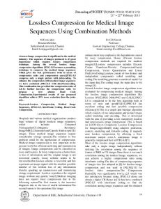
Fig. 1. An MRI-sequence

Fig. 2. Interframe correlation in the MRI-sequence

traframe prediction and interframe context-modeling. Due to the scheme’s simplicity, we are also guaranteed high processing speeds. A second scheme, based on JPEG-LS, is slightly more complicated. It exploits interframe redundancies the same way as the first scheme, and attains stateof-the-art compression ratios.

this finding can be the major source of improvement in an interframe approach. Previous frames can be used by an edge-detector for the current frame, allowing a more efficient coding of the edges. Considering the low overall correlation between successive frames, it can be expected that simple linear interframe prediction will not yield a better decorrelation than intraframe prediction. Techniques which exploit the edgeinformation from previous frames will not bother about the flat image regions (where almost no coding gain can be obtained), but will be able to code the edges better. In this case, the coding gain can be significant, as will be shown later.

II. I NTERFRAME CORRELATIONS In figure 1 an MRI-sequence is shown and in figure 2 the “local” correlations are visualized. A frame in figure 2 shows the local correlations between its corresponding frame in the original sequence and the corresponding frame’s previous frame. For each pixel, the local correlation is computed based on its eight closest neigbours in the current and previous frame (considering the raster-scan coding order, just as Interframe CALIC does). Higher intensities correspond with higher (absolute values of the) correlation. It can be seen that local interframe correlations are rather low in “flat” image regions (in which pixel intensities do not differ much) and that they are high at edges. In flat image regions, noise has a large influence on the local correlations. It is known that noise is very little correlated between successive frames, which is the main reason for the small correlation in the flat image regions. At edges, noise is less important and correlations tend to be larger (if the edges are not too much displaced between successive frames). From these results, some interesting conclusions can be drawn. Firstly, interframe redundancies are low in flat image regions. This is no real drawback as flat image regions can be coded very effectively using an intraframe approach. Secondly, the location (and sharpness) of edges can be predicted very well from the previous frame. As intraframe-only techniques have great difficulties coding edges efficiently (because the prediction errors are large),

III. O PTIMAL LINEAR PREDICTION n , where 1 ≤ h ≤ H, An image consists of pixels Ph,w 1 ≤ w ≤ W and 1 ≤ n ≤ N , and where H is the height and W is the width of a frame and N is the number of frames in the image. Prediction is based on a pixel’s closest neigbours in the current frame and the previous frames. Since the decoder must be able to reconstruct the prediction, only pixels can be used which are already coded and known to the decoder. We will refer to these “past” pixels as the coding history. When processing an image frameby-frame, and within a frame in raster-scan order, the coding history consists of all pixels in the previous frames and all pixels in the current frame which lie above the current pixel or to the left of the current pixel on the same line. The coding history is depicted in figure 3. It is obvious that not all pixels from the coding history are equally suitable for prediction. Only the pixels in a small neigbourhood from the current pixel can effectively contribute to the pixel’s prediction. In this paper, we will focus on simple linear predictors. Such a predictor is used in Lossless JPEG (LJPEG) [1], the current lossless compression standard for gray-scale

STW/SAFE99

Exploiting interframe redundancies in the lossless compression of 3D medical images x y

z

523

IV. JPEG-LS Frame n-2

11 00 00 00 00 00 00 0011 11 0011 11 0011 11 0011 11 0011 11 00 11 00 11 00 11 00 11 00 11 00 11 00 11 00 00 00 00 00 00 11 11 11 11 11 0011 11 0011 0011 0011 0011 00 Frame n-1 11 00 11 00 11 00 11 00 11 00 11 00 11 00 11 00 11 00 11 0011 11 00 000 111 00 11 00 11 00 11 00 11 00 11 00 11 000 111 00 11 00 11 00 11 00 11 00 11 00 00 00 00 00 00 1111 1111 11 11 11 00 11 00 00 11 00 11 00 11 00 11 000 00 11 00 11 00 11 00 11 00 11 111 Frame n 11 00 11 00 11 00 00 11 00 11 00 11 00 00 00 00 00 000 11 11 11 11 11 111 00 11 00 11 00 11 00 11 00 11 000 111 00 11 00 11 00 11 00 11 00 11 00 11 11 11 11 00 11 00 11 00 11 0000 11 00 000 111 00 11 000 111 00 11 00 11 00 11 00 11 00 11 00 00 00 00 11 11 11 00011 111 00 11 00 11 00 00 11 00 11 00 11 00 11 00 11 00 11 00 11 00 11 00 11 00 11 000 111 0011 11 0011 00 00 11 00 11 00 11 00 11 0011 11 00 11 00 11 00000 111 00 00 00 00 00 000 11 11 11 11 11 111 00 11 00 11 00 11 00 11 00 11 000 111 00 11 00 11 00 11 00 11 00 11 00 11 00 11 00 11 00 11 000 00 11 111 00 11 00 11 00 11 00 11 00 11 000 111 00 00 00 00 00 00 00 00 00 000 00 1111 1111 11 11 11 11 1111 11 11111 11 00 11 00 00 11 00 11 00 11 00 11 00 11 00 11 00 00 000 111 00 11 00 11 00 11 00 11 00 11 111 000 00 11 00 11 00 11 00 11 00 11 00 11 00 11 00 11 00 11 000 111 00 00 11 00 11 00 11 00 11 00 11 000 111 00 11 00 11 00 11 00 11 00 11 000 111 11111 00 11 00 11 00 11 00 11 00 11 00 11 00 11 00 11 00 11 000 00 11 000 111 00 11 00 11 00 11 00 11 00 11 00 11 00 11 11 00 00 11 00 11 00 11 00 11 00 11 00 11 000 111 00 11 00 11 00 11 00 11 00 11 00 11 00 11 00 11 00 11 00 11 000 111 00 000 00 11 00 11 00 11 00 11 00 11 111 00011 111 00 11 00 11 11 00 00 11 00 11 00 11 00 11 00 11 00 11 00 11 00 00 00 00 00 000 11 11 11 11 11 111 0 1 00 11 00 11 00 11 00 11 00 11 00 11 00 11 00 11 00 11 00 11 00 11 000 00 11 111 011 0011 0011 00 00 11 00 11 00 00 00 00 000 1100 111 11 11 1100 11 11100 11 00 11 00 11 00 11 0000 11 0000 11 00 11 00 11 00 11 00 11 00 11 00 11 00 00 00 1111 1111 11 11 00 11 00 00 11 00 11 00 11 00 11 00 11 00 11 ? 11 11 11 00 11 00 11 00 00 00 00 00 00 11 11 11 0 1 00 11 00 0 1111 111 00 00

Fig. 3. The already coded pixels form the coding history

images. In fact, the LJPEG-standard defines seven simple linear predictors, of which we will only consider the sevn denoting the current pixel, its prediction enth. With Ph,w n n is (Ph−1,w + Ph,w−1 )/2, where x denotes the largest integer not greater than x. This simple linear intraframe predictor will be the reference predictor when evaluating the interframe predictor. In order to be able to evaluate the full potential of linear prediction, an optimal predictor will be constructed. Given the pixels used in the prediction, optimal predictioncoefficients can be computed for a particular image. Although this is not feasible in practical compression schemes (because it is very time-consuming), the performance of the optimal predictors will give an idea of the obtainable coding gain. If no coding gain is obtained using the optimal predictors, non-optimal predictors will very probably not do better. The optimal linear predictor is  n P
h,w =

K  k=1

 ak Pk ,

JPEG-LS combines simplicity with the powerful compression potential of context-modeling. The JPEG-LS modeler/predictor processes the images in raster scan mode and has 2 basic modes of operation: “regular” mode and “run” mode. The latter is entered in smooth regions, where the limitations of its entropy coder (a Golomb-Rice coder) would force it to write at least one bit per pixel. However, coding runs of pixels as super-symbols allows the average number of bits per coded pixel to be less than 1. As far as lossless compression is concerned, most pixels are compressed using the “regular” mode; therefore, we will concentrate on this mode here. In a first step, the current pixel is predicted using the following non-linear n n , Ph−1,w and predictor that takes the gray values Ph,w−1 n Ph−1,w−1 of three neighbouring pixels as inputs, see table I. Even though this predictor is very simple, it deals appropriately with at least the most basic type of edges, i.e., horizontal and vertical ones. This predictor is called the “fixed predictor.” The context modeler of JPEG-LS not only provides information to the statistical coder but is also used to improve the prediction in a “level 2” step, which is called “adaptive correction”. The context modeler computes local gradient information and then uses this information to classify the current pixel into one of a number of classes. It also keeps an estimate of the mean prediction error within each class and subsequently adjusts the prediction error to obtain an unbiased estimate. It was experimentally observed that the resulting “level 2” prediction errors can be reliably modeled with a twosided geometric distribution (TSGD), which has only 2 parameters (the rate of decay and the mean value). This means that instead of estimating complete probability tables P(symbol|context) (for use in an arithmetic coder) for every possible symbol, the context modeler can simply estimate the 2 parameters of the TSGD. This has two important advantages: firstly, less memory is required to store 2 parameters than to store a probability table and secondly, the 2 parameters of the TSGD can be estimated much more reliably than a general probability table, especially in the early stages of coding when only a few pixels have been encoded. This improves the compression ratio.

where K is the number of pixels involved in the prediction. The pixels Pk (1 ≤ k ≤ K) are part of the coding n . The predictionhistory of the pixel to be predicted Ph,w coefficients ak will be computed based on the correlations between the pixels Pk in the image. Because minimization of the compressed code-length cannot easily be done, the coefficients will be optimized such that the variance of the prediction error is minimal. V. I NTERFRAME CONTEXT- MODELING The prediction errors will not be entropy-coded. Rather, the remaining entropy after (predictive) decorrelation is In the non-linear approach, prediction is purely incomputed. These entropy figures will be very close to traframe (using the simple LJPEG-predictor or the more the actual code-lengths obtainable by state-of-the-art arith- complicated two-step JPEG-LS predictor, see fig. 4). Inmetic coders [13–15]. terframe redundancies are exploited by interframe context-

IEEE/ProRISC99

Steven Van Assche et al.

524

 n n n n n if Ph−1,w−1 ≥ max(Ph,w−1 , Ph−1,w )  min(Ph,w−1 , Ph−1,w ) n n n n n n
max(Ph,w−1, Ph−1,w ) if Ph−1,w−1 ≤ min(Ph,w−1 , Ph−1,w ) Ph,w =  n n n Ph,w−1 + Ph−1,w − Ph−1,w−1 otherwise TABLE I P REDICTOR USED IN JPEG-LS

modeling. The context for the current pixel is formed by the magnitude of the prediction error for the corresponding pixel in the previous frame. Note that this prediction error comes from the intraframe prediction step in the previous frame. In the following, we will refer to it as the reference frame prediction error.

Image MRI T1 MRI T2 MRI PD CT

Size of a frame 256 × 256 256 × 256 256 × 256 512 × 512

Number of frames 293 315 377 1734

TABLE II

The contexts hold counts of intraframe prediction erI MAGES USED IN THE EVALUATION ror/reference frame prediction error pairs. In practical compression schemes, these counts drive an entropycoder. As mentioned above, we will do no actual codTechnique Predictor ing, but we will only compute the remaining entropy. n n LJPEG (Ph−1,w + Ph,w−1 )/2 The main asset of context-modeling lies in its ability to n−1 n n LJPEG-3D/opt a1 Ph−1,w + a2 Ph,w−1 + a3 Ph,w  separate statistics. In our case, intraframe prediction errors are coded conditioned on the corresponding reference TABLE III frame prediction errors. If there exists a good correlaE VALUATED LINEAR PREDICTORS tion between the reference frame prediction errors and the intraframe prediction errors, context-modeling will provide conditional statistics which are very well suited for5 statistics. This is necessary because large intraframe preentropy-coding. diction errors are far less frequent than small errors. In our case, the context-modeling step serves as edgedetector: the magnitude of the reference frame prediction VI. E XPERIMENTAL RESULTS errors indicate the presence and sharpness of edges. As We will evaluate the different techniques on four threefound in section II, there exists a strong correlation bedimensional medical images: three MRI-images and one tween edges in successive frames. Therefore, we expect the interframe context-modeling step to be very beneficial CT-image. These images originate from the Visible Hufor coding because the intraframe prediction error statis- man Project (VHP) [16], in this case the female corpus. tics from flat and edgy image regions will be separated. Their sizes are shown in table II. All four images have 12 In flat image regions (small reference frame prediction er- bits per pixel (bpp). rors), intraframe prediction is adequate and intraframe prediction errors are very small. The statistics will not be dis- A. Optimal linear prediction torted by the generally much larger prediction errors comThe linear predictive techniques which will be evaluated ing from edgy image regions. On the other hand, statistics are shown in table III. It is supposed that pixel Pn is to h,w in edgy image regions will also be more reliable: large in- be predicted. LJPEG is the reference predictor. LJPEGtraframe prediction errors will be more probable than small 3D/opt uses a current pixel’s three closest pixels in the errors, which is certainly not the case in the flat image re- prediction: the pixels from the LJPEG-prediction and its gions. corresponding pixel in the previous frame. This is the When forming the context, reference frame prediction errors are grouped into bins depending on their magnitude. The bins are chosen larger for large reference frame prediction errors in order to make it possible for the contextmodeling step to gather sufficient counts and build reliable

most straightforward interframe extension of the LJPEGstandard predictor. Note that, as the correlation between frames in medical images drops off rapidly for more distant frames, only one previous frame is used in the interframe prediction.

STW/SAFE99

Exploiting interframe redundancies in the lossless compression of 3D medical images

525

INTRA-FRAME CONTEXT MODEL

Current Frame

INTER-INTRA CONTEXT MODEL

Determine Intra-frame Context

Real Pixel Value

Error Feedback

+ -

Reference frame residuals

INTRA

Predict

Residual

INTER

Entropy coding using selected statistics

Coded bits

Quantize

MOST INFORMATION RETRIEVAL ACTIONS ARE SHOWN INFORMATION UPDATES ARE NOT

Fig. 4. Overview of the 3D JPEG-LS scheme

Image MRI T1 MRI T2 MRI PD CT

Original 12 12 12 12

LJPEG 5.23 5.03 5.41 5.88

LJPEG-3D/opt 5.19 5.00 5.39 5.79

TABLE IV R ESULTS FOR THE LINEAR PREDICTORS

The results for the linear predictors from table III, are shown in table IV. The figures given are remaining entropies after predictive decorrelation, expressed in bit per pixel. It can be seen that the interframe predictors do not yield any noteworthy compression improvement. interframe redundancies in medical images can thus clearly not be exploited by linear prediction. In table V, the optimal coefficients are shown for the LJPEG-3D/opt predictor. For the MRI images, the intern−1 frame pixel (Ph,w ) makes only a very minor contribution to the prediction. From this, it can easily be understood that the linear interframe prediction does not work. It is remarkable that for the CT image, the reference frame pixel does add to the prediction. This is probably due to the fact that CT images mostly contain far less noise than MRI im-

IEEE/ProRISC99

Image MRI T1 MRI T2 MRI PD CT

Optimal predictor n−1 n n 0.21Ph−1,w + 0.75Ph,w−1 + 0.03Ph,w n−1 n n 0.27Ph−1,w + 0.68Ph,w−1 + 0.05Ph,w n−1 n n 0.22Ph−1,w + 0.75Ph,w−1 + 0.03Ph,w n−1 n n 0.46Ph−1,w + 0.21Ph,w−1 + 0.33Ph,w

TABLE V O PTIMAL COEFFICIENTS FOR LJPEG-3D/ OPT

ages. Nevertheless, the additional decorrelating potential of the interframe pixel is not sufficient to provide a clearly better linear prediction. B. Interframe context-modeling In table VI, the results are shown for the techniques using interframe context-modeling. As can be seen, the non-linear approach does yield a compression improvement. Compressed bitrates drop by about 5 to 10%. As the implemented context-modeling is very simple, higher gains can be expected from more complex non-linear approaches. In fig. 5, a comparison is shown of JPEGLS/CM, JPEG-LS and CALIC on the CT image. In this figure, every frame is compressed using its previous frame as reference frame. For most frames, JPEG-LS/CM per-

Steven Van Assche et al.

526 Image MRI T1 MRI T2 MRI PD CT

Original 12 12 12 12

LJPEG 5.23 5.03 5.41 5.88

LJPEG/CM 5.02 4.86 5.16 5.41

JPEG-LS 4.63 4.52 4.79 4.80

JPEG-LS/CM 4.40 4.31 4.61 4.42

TABLE VI R ESULTS FOR THE INTERFRAME CONTEXT- MODELING APPROACH

6.0

R EFERENCES JPEG-LS (3D) JPEG-LS (2D) Calic (2D)

[1]

[2]

bit per pixel

5.0

[3]

4.0

[4]

[5] 3.0 0.0

500.0

1000.0 frame number

1500.0

2000.0

Fig. 5. Comparison of JPEG-LS/CM with CALIC and JPEGLS on the CT image from the VHP (female) data set

[6]

[7]

forms better than the intraframe techniques, but for some [8] others, its performance is worse. It is not clear why this [9] happens. VII. C ONCLUSION

[10]

In this paper the suitability of three-dimensional predictive techniques for lossless compression of medical images is investigated. It is shown that linear interframe prediction does not provide a better decorrelation than two- [11] dimensional intraframe prediction. It is demonstrated that the use of a non-linear interframe decorrelator (in this case [12] context-modeling) does yield higher compression. With a simple technique, a decrease in compressed bitrate of about 10% could be noted. [13]

ACKNOWLEDGMENTS This work was financially supported the Flemish Insti- [14] tute for the Advancement of Scientific-Technological Research in Industry (IWT) through the projects Tele-Vision [15] (IWT 950202) and Samset (IWT 950204).

The International Telegraph and Telephone Consultative Committee (CCITT), Eds., Digital Compression and Coding of Continuous-Tone Still Images, Recommendation T.81, 1992. G.K. Wallace, “The JPEG still picture compression standard,” Communications of the ACM, vol. 34, no. 4, pp. 30–44, Apr. 1991. Stephane G. Mallat, “A theory for multiresolution signal decomposition: The wavelet representation,” IEEE Transactions on Pattern Analysis and Machine Intelligence, vol. 11, no. 7, pp. 674– 693, July 1989. X. Wu, N. Memon, and K. Sayood, “A context-based, adaptive lossless/nearly-lossless coding scheme for continuous-tone images,” Proposal for the initial ISO/JPEG evaluation, juli 1995. Xiaolin Wu, Wai-kin Choi, and Nasir Memon, “Lossless interframe image compression via context modeling,” in Proceedings of the Data Compression Conference, J. A. Storer and M. Cohn, Eds., Snowbird, Utah, USA, Mar. 1998, IEEE Computer Society, pp. 378–387. John A. Robinson, “Efficient general-purpose image compression with binary tree predictive coding,” IEEE Transactions on Image Processing, vol. 6, no. 4, pp. 601–608, Apr. 1997. John A. Robinson, “Binary tree predictive coding,” http://monet.uwaterloo.ca/ john/btpc.html, 1995. “JPEG-LS source code, v.2.1,” http://www.jpeg.org. M. Weinberger, G. Seroussi, and G. Sapiro, “The LOCO-I lossless image compression algorithm: Principles and standardization into JPEG-LS,” Tech. Rep. HPL-98-193, HP Computer Systems Laboratory, Nov. 1998, http://www.hpl.hp.com/techreports/98. K. Denecker, S. Van Assche, W. Philips, and I. Lemahieu, “State of the art concerning lossless medical image coding,” in Proceedings of the PRORISC IEEE Benelux Workshop on Circuits, Systems and Signal Processing, J.-P. Veen, Ed., Mierlo, NL, Nov. 1997, STW Technology Foundation, pp. 129–136. P. Roos and M.A. Viergever, “Reversible 3-d decorrelation of medical images,” IEEE Transactions on Medical Imaging, vol. 12, no. 3, pp. 413–420, Sept. 1993. S. Van Assche, K. Denecker, W. Philips, and I. Lemahieu, “Lossless compression of three-dimensional medical images,” in Proceedings of the PRORISC IEEE Benelux Workshop on Circuits, Systems and Signal Processing, J.-P. Veen, Ed., Mierlo, NL, Nov. 1998, STW Technology Foundation, pp. 549–553. Paul G. Howard and Jeffrey Scott Vitter, “Arithmetic coding for data compression,” Proceedings of the IEEE, vol. 82, no. 6, pp. 857–865, June 1994. Jr. Glen G. Langdon and Jorma Rissanen, “Compression of blackwhite images with arithmetic coding,” IEEE Transactions on Communications, vol. COM-29, no. 6, pp. 858–867, June 1981. W. B. Pennebaker, J. L. Mitchell, Jr. G. G. Langdon, and R. B. Arps, “An overview of the basic principles of the Q-coder adap-

STW/SAFE99

Exploiting interframe redundancies in the lossless compression of 3D medical images tive binary arithmetic coder,” IBM Journal of Research and Development, vol. 32, no. 6, pp. 717–726, Nov. 1988. [16] National Library of Medicine, Visible Human Project, http://www.nlm.nih.gov/research/visible/getting data.html. [17] D. De Rycke and W. Philips, “Lossless non-linear predictive coding of video data through context matching,” in The 5th International Conference on Information Systems Analysis and Synthesis (ISAS’99), M. Torres, B. Sanchez, and D.G. Langlois, Eds., Aug. 1999, pp. 42–49, Orlando.

IEEE/ProRISC99

527

This page was intentionally left blank