Exploiting Local Similarity for Indexing Paths in Graph-Structured Data Pradeep Shenoy∗
Raghav Kaushik∗
Philip Bohannon
Ehud Gudes∗
University of Wisconsin
University of Washington
Bell Laboratories
Ben-Gurion University
[email protected]
[email protected]
[email protected]
[email protected]
Abstract XML and other semi-structured data may have partially specified or missing schema information, motivating the use of a structural summary which can be automatically computed from the data. These summaries also serve as indices for evaluating the complex path expressions common to XML and semi-structured query languages. However, to answer all path queries accurately, summaries must encode information about long, seldom-queried paths, leading to increased size and complexity with little added value. We introduce the A(k)-indices, a family of approximate structural summaries. They are based on the concept of k-bisimilarity, in which nodes are grouped based on local structure, i.e., the incoming paths of length up to k. The parameter k thus smoothly varies the level of detail (and accuracy) of the A(k)-index. For small values of k, the size of the index is substantially reduced. While smaller, the A(k) index is approximate, and we describe techniques for efficiently extracting exact answers to regular path queries. Our experiments show that, for moderate values of k, path evaluation using the A(k)-index ranges from being very efficient for simple queries to competitive for most complex queries, while using significantly less space than comparable structures.
1. Introduction With the rapidly increasing popularity of XML for data representation, there is a lot of interest in query processing over data that conforms to a labeled-tree or labeledgraph data model. A schema for such data, if present, may only partially constrain the data. For example, in XML Schema [31], the construct allows arbitrary content to appear under a given element. As a result, several techniques have been developed to extract structural summaries directly from the data [13, 14, 15, 22, 23]. By aiding the user in query formulation and serving as a convenient place to store statistics [14], a structural summary can fulfill many ∗ This work was conducted in part while the author was visiting Bell Labs.
of the roles of the schema in a traditional database, but, unlike a schema, it is not prescriptive and thus may change with any update. Structural summaries can also play an important role in query evaluation for graph-structured data, even when a schema is present. In each of the many query languages proposed for querying such data [1, 5, 9, 10, 11, 27], the relatively simple FROM clause of SQL has been replaced by a pattern language [12] built around path expressions. While simple path expressions were popularized in objectoriented query languages, most path languages proposed for semistructured, XML, or graph-structured data are substantially more complex, using either regular path expressions [5, 27] or XPath [7] expressions [6, 9]. Efficient query answering in these languages clearly depends on efficient evaluation of complex path expressions. Structural summaries of semi-structured data aid in this evaluation by pruning the search space. Alternatively, an index graph, consisting of a structural summary along with a stored mapping from summary nodes to data nodes, may be used to evaluate such path expressions [14, 21] directly. This paper introduces the A(k)-indices, a family of efficient, flexible data structures capable of serving as structural summaries of—or index graphs for—graph-structured data. The key observation exploited by the A(k)-indices is that not all structure is interesting. In particular, long and complex paths tend to contribute disproportionately to the complexity of an accurate structural summary [15]. The A(k)indices become approximate for paths longer than k, thus exploiting the similarity of short paths to reduce the size of the structure. The A(k)-index is substantially smaller than a fully accurate structure, substantially faster for shorter path expressions and, surprisingly, quite competitive for arbitrary path expressions. Beyond the introduction of the A(k)-index, this paper makes two key contributions. First, we develop efficient techniques for extracting exact answers to path expressions from approximate index graphs. These include techniques for validating nodes which are in-doubt and observations allowing a number of needless validations to be avoided. Second, we report the results of a preliminary study of perfor-
mance which addresses (1) the comparative performance of the A(k)-index, the 1-Index [21] and the original data graph on two real-world data sets, and (2) the impact of the parameter k on the size of the index graph and performance. Our performance results show that the A(k)-indices are spaceefficient and effectively support path queries. For example, on a large classes of “simple” queries evaluated on a subset of the Internet Movie Database [30], using the A(3)-index reduces query processing cost (measured in graph-node visits) by around 47% compared to the 1-Index. On the same data set, the A(3)-index is much smaller than the 1-Index with 62% fewer nodes. The rest of the paper is organized as follows. Background material is presented in Section 2. In Section 3, we introduce the A(k)-index and its construction algorithm. Section 4 introduces techniques for path-expression evaluation, and Section 5 evaluates the search performance of the A(k)-index. We discuss related work in Section 6 and conclude in Section 7.
2. Background We model XML or other semi-structured data as a directed, labeled graph G = (VG , EG , root, ΣG , label , oid , value). Each edge in EG indicates an object-subobject or objectvalue relationship. “Simple” nodes in VG have no outgoing edges and are given a value via the value function. Each node in VG is labeled with a string-literal from ΣG via the label function and with a unique identifier via the oid function, with simple objects given the distinguished label, VALUE. There is a single root element with the distinguished label, ROOT. Example 1: Figure 1 shows a portion of a hypothetical “metro-guide”, represented as a data graph. In the figure, the numeric identifiers in nodes represent oid ’s. Such a guide could reasonably be built from a collection of XML documents published by businesses, civic groups and other interested parties. Non-tree edges may be implemented with the ID / IDREF construct or XLink [29] syntax. We now introduce some terminology about paths and path-expressions. A node path in G is a sequence of nodes, n0 . . . np such that an edge exists between node ni and ni+1 , for 0 ≤ i ≤ p − 1. A label path is a sequence of labels l0 . . . lp , and a node-path matches a label path if label(ni ) = li , for 0 ≤ i ≤ p. A path (if not specified, a path refers to a label path), l0 . . . lp , matches (or is valid for) a node n if l0 . . . lp matches a node path ending in n. A k-path is a path with p ≤ k. A simple path expression is a label path in which the first label is ROOT. A regular path expression, R, is defined in the usual way in terms of sequencing (.), alternation (|), repetition (∗) and optional expressions (?), as shown below. R ::= ΣG | | R.R | R|R | (R) | R? | R∗
The symbol matches any li ∈ ΣG . Path expressions always begin by matching the root element of the database graph, and the initial ROOT label is implied if omitted. We denote by L(R), the regular language specified by R. We say that R matches a data graph node n, if some label path appearing as a word in L(R) matches some node path ending in n. The result of evaluating R on G is the set of nodes in VG which match R. For example, the simple path expression, ROOT.metro.cultural.museum, evaluated on the graph in Figure 1, would return {6,7}. The following, more complicated expression finds the names of hotels or museums in Westside or Northside: ROOT.metro.neighborhoods.neighborhood.( | . )?. (hotel|museum).name. This expression matches the nodes {12,14,16,19}. Here, the optional | . allows the query to ignore irregularities in the schema, such as the use of attraction.cultural tags for museums but just a hotels tag for hotels. Another common class of queries includes an initial ∗ ; for example, ∗ .hotel finds all hotel nodes in the graph. The need to create a structural summary for semistructured data was clearly identified in the Lore project [18], and the DataGuide was created in response [14, 23]. The approach taken by the dataguide, and followed by other work including this paper, is to create a structural summary in the form of another labeled, directed graph. The idea is to preserve all the paths in the data graph in the summary graph, while having far fewer nodes and edges. As proposed in [14, 21], it is possible to associate an extent with each node in the summary to produce an index graph. If A is a node in the index graph I(G), then ext I (A), the extent of A with respect to I(G), is a subset of VG . The index graph result of executing a path expression R on I(G) is the union of the extents of the index nodes that match R. We require that the extent mapping be safe: if l0 .l1 . . . lk is a label path which matches a path to node v in G, then there must be some node A in I(G) for which l0 .l1 . . . lk matches a path to A and v ∈ ext I (A). This guarantees that the result of any path expression R on G is contained in the result of R on I(G). An index graph is said to be precise if the converse also holds; that is, if v ∈ ext I (A) and l0 .l1 . . . lk is a valid label path for A, then l0 .l1 . . . lk is a valid label path for v. We now define the notion of bisimilarity [26], since it is closely related to the A(k)-index. A symmetric, binary relation ≈ on VG is called a bisimulation if, for any two data nodes u and v with u ≈ v, we have that (a) u and v have the same label, and (b) if u0 is a parent of u, then there is a parent v 0 of v such that u0 ≈ v 0 , and vice-versa. Two nodes u and v in G are said to be bisimilar, denoted by u ≈b v, if there is some bisimulation ≈ such that u ≈ v. For example, in Figure 1, objects 8 and 9 (the hotel nodes) are
ROOT
1
metro
2
3
6 12
name
cultural
museum 13
phone
7 14
4
museum
name 15 phone
8 16
business
hotel
9
name
5
hotel 19
10
name
neighborhoods
neighborhood
20
22
11
name
neighborhood 24
name
hotels "6615887" "Museum of Natural History"
"Museum of Art"
"2319837"
"Hilton"
"Sheraton"
"Northside" 21
17
nearby
18
attraction
"Westside" 23
attraction
nearby
25
cultural 26
cultural
Figure 1. An example graph-structured database bisimilar, while objects 21 and 23 (labeled attraction) are not, since 21 has a parent labeled nearby. By extension, objects 25 and 26 (the nodes immediately below them, labeled cultural) are also not bisimilar, since they have nonbisimilar parents. An easy induction shows that if two nodes are bisimilar, the set of in-coming paths into them is the same. The partition of VG induced by ≈b can be used to obtain an index graph by creating an index node for each equivalence class and setting the members of the equivalence class as the extent of the node. An edge is added from index node A to B when an edge exists in G from some node u in ext[A] to a node v in ext[B]. This is one way of defining the 1-Index [21]1 . This index graph is referred to as Bisim(G) or simply “the 1-Index” in this paper. Thus, there is a worst case guarantee on the index size, since the 1-Index can never be bigger than the data graph. Further, it can be computed in time O(m lg n) where n is the number of nodes and m is the number of edges in the data graph, using an algorithm proposed by Paige and Tarjan [25].
3. The A(k)-index The 1-Index and the DataGuide precisely encode all paths in the data graph, including long and complex paths. Thus, even when two nodes are locally similar, they may be stored in different extents due to a variety of complex and/or circuitous paths. For instance, in the example in Figure 1, the subtrees rooted at 6 and 7 appear similar. But, they are not bisimilar due to the incoming path to 6 that passes through hotel.nearby.attraction.cultural. Even in this small example, it is clear that this path may not be very important for querying museum objects. It is easy to get longer paths with even less semantic content in larger examples, and 1 The
authors of [21] also consider the use of the similarity relationship for the 1-Index. We do not consider this alternative due to inefficient construction algorithms for the similarity relation – see [21] for details.
when many such paths exist, the 1-Index can be close to the data graph in size. In fact, on a subset of the data from the Open Directory Project (see Section 5), the 1-Index turns out to be about 45% of the data graph size. Of course, if these long and complex paths are key to the majority of queries written by users, then the larger 1Index may be preferred. However, we expect such queries to be rare in practice. Based on this intuition, we explore the problem of building index graphs that take advantage of local similarity, in order to reduce the size of the index graph. By this, we mean that nodes with similar structure, for example the museum nodes of Figure 1, should be grouped together as much as possible, even if there is some long path (in this case through the hotels) which distinguishes them. To accomplish this goal, we exploit the fact that any equivalence-class partition of the nodes of the data graph can be used to create an index graph by a process similar to the one for the 1-Index. Any such index graph is safe and is never larger than the data graph in size; however, such an index graph may not be precise. To illustrate this point, the index graph obtained by simply classifying the nodes of the graph shown in Figure 1 by label is shown in Figure 2(a). In this figure, the labels associated with the index nodes correspond to the common label of the data nodes in their extents. The numbers shown beside the index nodes are the oid s of the data nodes in the respective extents. We first note that the index graph has combined the subtrees starting from nodes labeled cultural and business, respectively. This is certainly an acceptable approximate summary for the original database. However it does have false paths: e.g., the museum node with oid 7 is not reachable from any node labelled hotel in the original database. Consider further the index graph in Figure 2(b). This is a more detailed index graph with the following special property: there are no false paths of length 2 (length measured
1
ROOT
2
metro 3
cultural
4
6,7
museum
8,9
phone
12,14,16 19,22,24
3,25,26
business
neighborhoods
5
cultural
13,15
name 17,18
neighborhood
10,11
20
nearby
13,15
metro
phone
neighborhoods
5
hotel
8,9
10,11
20
neighborhood
hotels
22,24
name
23
attraction
26
cultural
name
16,19
21
attraction
25
cultural
nearby
17,18
hotels 21,23
2
name
12,14
hotel
ROOT
business
4
museum
6,7
1
attraction
(a) (b) Figure 2. Two index graphs for the data graph in Figure 1 in terms of number of edges) in the index graph. For example, the nodes 25 and 26 are now separated, because of the 2-length path nearby.attraction.cultural into node 25. We could go further by splitting the node containing 6 and 7 in its extent to ensure that all paths of length 3 were valid. We formalize this process to obtain a family of index graphs. The main idea of these structures is to give up absolute precision and group similar pieces of data together in order to allow the index size and the maximum area of the index graph affected by an update to be controlled by the parameter k, which is set to 2 in Figure 2(b). As the parameter increases, indices in the family get more and more accurate, finally equaling the 1-Index.
3.1 An Index-Graph Based on k -Bisimilarity As a step towards achieving the goal of indexing the “desirable” paths of a data graph, we propose the A(k)-index which classifies data graph nodes based on paths of length k entering these data nodes. We obtain the A(k)-index using the notion of k-bisimilarity [20], which satisfies the property: if two nodes u and v are k-bisimilar, then the set of k-paths into these nodes is identical. Definition 1: ≈k (k-bisimilarity): This is defined inductively. 1. For any two nodes, u and v, u ≈0 v iff u and v have the same label. 2. Node u ≈k v iff u ≈k−1 v and for every parent u0 of u, there is a parent v 0 of v such that u0 ≈k−1 v 0 , and vice versa. By a simple induction, we can see that this definition ensures the weaker condition it sets out to achieve. Note that k-bisimilarity defines an equivalence relation on the nodes of a graph. We call this the k-bisimulation. We can obtain an index graph from the k-bisimulation by creating an index node for each equivalence class and associating the data nodes in the class to the extent of the node. Edges are added by a process similar to the one for the 1-Index,
explained in Section 2. We call this the A(k)-index. Increasing k refines the partition induced by this equivalence relation by splitting certain equivalence classes. This continues until a fixed-point is reached, at which the relation can be shown [20] to be exactly the (maximal) bisimilarity relation from which Bisim(G) (the 1-Index) is derived. This process is illustrated in Example 2. 1
1
A
2 B
3
C
4 D
5
D
4,5
D
6 E
7
E
6,7
E
G
2
A
B
3
A(0)
1
A
1
A
C 2
B
3
C 2
B
3
C
4
D
5
D 4
D
5
D
6,7
A(1)
E
6
E
7
E
A(2)=1-index
Figure 3. A Sequence of A(k)-Indices Example 2 Figure 3 shows a data graph and its A(0)index, A(1)-index and A(2)-index based respectively on 0bisimilarity, 1-bisimilarity and 2-bisimilarity. In this case, the 2-bisimulation is actually the maximal bisimulationbased 1-Index. We also note that the index graphs shown in Figures 2(a) and 2(b) are the A(0)-index and the A(2)-index respectively for the data graph shown in Figure 1. This illustrates how the family of A(k)-indices can be used to pick a structural summary with a requisite amount of detail, or which meets a given space constraint. We now describe, without proof, some properties of these index graphs. Property 2: (a) If nodes u and v are k-bisimilar, then the set of labelpaths of length ≤ k into them is the same. (b) The set of label-paths of length k into an A(k)-index node is the set of label-paths of length k into any node in its extent.
(c) The A(k)-index is precise for any simple path expression of length less than or equal to k. (d) The A(k)-index is safe, i.e., its result on a path expression always contains the graph result for that query. (e) The (k + 1)-bisimulation is either equal to or is a refinement of the k-bisimulation. From Property 2(a), one can see that by varying k, we obtain a smooth range of A(k)-indices that increase in size and converge to the 1-Index. Further, by Property 2(e) each subsequent index is derived by splitting some of the nodes in the previous index. This is the intuition behind the index construction algorithm described in the next section. Finally, we present a property of the A(k)-index which limits the impact of an update on the index graph. Unlike the 1Index, the effect on the index of any update in the data graph is limited locally to a “neighborhood” of distance k, as formalized by the following property: Property 3: Let v, x, y be three nodes such that the shortest path to x from v or to y from v contains more than k edges. If an edge is added or deleted going from a node u to v, this update does not affect the k-bisimilarity relationship between x and y.
3.2 A(k )-index Construction The algorithm to compute the A(k)-index is a variant of the standard algorithm [25] for computing the bisimulation. Before presenting the construction algorithm, we introduce the important notion of the stability of one set of graph nodes with respect to another. For a set of nodes, A, let Succ(A) denote the set of successors of the nodes in A, i.e., the set {v| there is a node u ∈ A with an edge from u to v}. Definition 4: Given two sets of data graph nodes A and B, A is said to be stable with respect to B if either A is a subset of Succ(B) or A and Succ(B) are disjoint. Let us call a partition, P1 , of VG stable with respect to partition P2 of VG if each equivalence class in P1 is stable with respect to every class in P2 . Then, the (k + 1)bisimulation is the coarsest refinement of the k-bisimulation that is stable with respect to it. If we have two sets of nodes (or node-sets), A and B, and we wish to make A stable with respect to B, we split A into A ∩ Succ(B) and A − Succ(B). We represent the k-bisimulation by a list of node-sets, each of which corresponds to one equivalence class in the k-bisimulation partition, and compute the (k + 1)-bisimulation in two steps. First, we make a copy of the k-bisimulation and then we split the equivalence classes (node-sets) in this copy until they are stable with respect to the equivalence classes of the k-bisimulation. The procedure compute k bisim is sketched in Figure 4. The data structures used to implement this efficiently are based on the ones used in [25]. The algorithm maintains a partition
of the data nodes, Q, as a list of node-sets. In each iteration, the algorithm stabilizes Q with respect to a copy of itself (line 8 implements stabilization of one node-set w.r.t another). This process is repeated k times. Thus, if the initial partition is one by label, i.e is the A(0)-index partition, then the algorithm outputs the partition corresponding to A(k)index. In the figure, X is set to a copy of the Q partition. This approach takes time O(km) and space O(m), where m is the number of edges in G. Once the k-bisimulation partition is computed, the A(k)-index is constructed by the procedure compute A(k) index as shown in Figure 4.
3.3 Index Composition and the Label Map Unlike a value-based index like a hash table, index graphs are themselves data graphs, and in most cases, any path index which can be maintained on a data graph can be maintained and used on an index graph. Given a variety of possible index structures, their composition leads to a large index design space and corresponding path evaluation search space, both of which are beyond the scope of this paper. For this work, we consider only one composition: the addition of a label-map. The label-map is simply a partition of data nodes by label, analogous to the “edge index” of [19], and allows access to nodes with a certain label. It is implemented as a hash table (We consider it unlikely that any large data graph would be stored without such an mapping, and data nodes may even be stored clustered by label).
4. Path Evaluation with Approximate Index Graphs In this section we present our strategies for data graph and index graph search, introduce our validation-based techniques for path evaluation on approximate indices, and present a technical result which allows unnecessary validations to be avoided.
4.1 Path Expression Evaluation We evaluate a path expression R on a graph with either a forward or a backward strategy. The forward strategy simply involves simulating the action of an NFA on the graph as described below. A backward evaluation strategy for R makes use of the label-map, introduced in 3.3, to find the nodes bearing the final label(s) mentioned in R. Then R is evaluated in a reverse manner from these nodes to determine whether any paths to these data nodes match the automaton. The intuition here is that the “end” of the expression may be significantly more selective than the earlier parts, and thus processing in this manner could be cheaper. Note however that this is an optimization issue, and depending on the data and query (as we shall see), either one of forward and backward executions may be better. One purpose of evaluating multiple search techniques, including the use of the label-map, is to avoid certain very
procedure compute k bisim(G,k) begin 1. Q and X are each a list of node-sets 2. Q = partition VG by label 3. X = (a copy of) Q 4. for i = 1 to k do 5. foreach X in X do //stabilize Q w.r.t X 6. compute Succ(X) 7. foreach Q in Q do // split 8. replace Q by Q ∩ Succ(X) and Q − Succ(X) 9. if there was no split then 10. break 11. X = (a copy of) Q end
procedure compute A(k) index(G, k) begin 1. compute k bisim(G,k) 2. foreach equiv. class in k-bisimulation do 3. create an index node I 4. ext[I] = data nodes in the equiv. class 5. foreach edge from u to v in G do 6. I[u] = index node containing u 7. I[v] = index node containing v 8. if there is no edge from I[u] to I[v] then 9. add an edge from I[u] to I[v] end
Figure 4. A(k)-index computation poor evaluation strategies. For example, an initial ‘ *’ construct is commonly used to find a pattern anywhere in the graph, yet with the naive automaton-based execution scheme the entire graph will be explored with this pattern. Thus, we use the label-map to begin evaluation with the first non-wildcard labels in the query. There are many other feasible execution plans, but their evaluation is beyond the scope of this paper. Forward evaluation of regular path queries on a graph proceeds as follows: 1. an NFA, A, is created according to the regular expression P = ROOT .R. 2. A is then run on the index graph, i.e., the index graph is traversed breadth-first, while making corresponding state transitions in the automaton for matching (nodelabel, transition-label) pairs. 3. A table is kept to avoid repeatedly visiting a data node in the graph in the same state of the automaton, thus avoiding cycles. 4. When a node in the index graph is reached while the corresponding automaton state is an accept state, the index node is added to the final result. Note that due to the table above, each edge is visited only once in each state, and thus the cost of evaluation is limited to O(|A|m) where |A| is the number of states in automaton A and m is the number of edges in the graph. For practical queries, |A| is a small constant.
4.2 Handling Approximate Index Graphs To evaluate a regular expression R on an index graph, we simply use the (forward or backward) automaton evaluation strategy above, but adding the nodes in ext[B] rather than B itself to the result set when B is accepted by the automaton. Since our indices are safe, the A(k)-index result set for R always is a superset of the target set (i.e., the results obtained on the data graph). Further, by Property 2(c), when the automaton execution strategy above accepts a node, B, in the A(k)-index graph along a path of length ≤ k from the
root, a node in ext[B] must be in the target set of R. When an index node is accepted by a longer path, the data nodes are initially added to a “maybe-set”, M , instead of the result set (By exploring the graph breadth-first, we ensure that the shortest path to a node is found first). We deal with the possible false positives by validating the nodes of M against the original data graph. This validation is handled by a reverse execution of the automaton on the data graph beginning with each node in M . While this is potentially expensive, we take advantage of shared paths to mitigate the expense. The idea is to keep track, for any node passed on the way to an accept state in the reverse execution, which state the automaton was in at that node. Later, if the node is encountered again in the same state, we know the validation leads to a “yes” answer, and can terminate the current automaton execution. A similar technique, with minor modifications, can be used to keep track of paths that lead to failure as well. Note that using the backward evaluation strategy on the data graph and the validation of “maybe” nodes are closely related. The main difference is the number of nodes which must be checked using the reverse automaton. In fact, a backward evaluation strategy on the data graph will usually need to do a backward traversal from more nodes than the A(k)-index validation. This is because the A(k)-index provides better pruning than a simple label-map, at the cost of visiting nodes in the A(k)-index to achieve this pruning.
4.3 Avoiding Needless Validation We now prove a theorem that significantly reduces the need to validate nodes by allowing node extents to be marked directly as valid. Consider a label-path p = l1 , l2 , . . . , lj , j ≤ k and an A(k)-index node N , such that p is the suffix of one or more paths to N . For path expression P , let L(P ) denote the associated regular language. Theorem 1: If all paths p0 .p that exist in the database are in L(P ) for a path expression P , then all data-graph nodes in the ext[N ] are in the target set of P .
The proof of Theorem 1 appears in the full version of the paper [4]. To illustrate the idea behind Theorem 1, consider evaluating two path expressions, • bad =A.B.D.E and • good =A.(B|C).D.E evaluated on the A(1)-index shown in Figure 3. Upon arriving at oid 7 in the index when evaluating good , we can conclude that it is a valid member of the answer set and need not be validated, even though it is at distance 3 from the root along the path we matched. The reason is as follows: (1) Since the A(1)-index is accurate for the suffix D.E of the path into the data graph node 7, the existence of a parent with label D (in this case, node 5), is ensured, (2) node 5 is connected to the root, and so there is a path with suffix D.E into node 7, (3) every path ending in D.E in the database is matched by this query and hence (4) node 7 is in the result set of this query. Since this is not the case for bad , node 7 must be validated (and in this case will be discarded from the exact answer). Our current implementation takes advantage of Theorem 1 in only two cases. First, we disregard the distinguished root of the graph, since our data files are drawn from XML where each document has a single root (and thus all paths go through that root also). Second, we make use of the subcase where the path expression is of the form ∗ .R, a common construct. That is, if a node N in an index graph is recognized by an automaton due to some path p, the portion of p that was matched by the ∗ trivially satisfies the condition of Theorem 1, and thus only the length of the portion of the path matched by R need be considered. The result of these observations is that many simple queries can be evaluated accurately on the A(k)-index, and this fact is demonstrated on queries on real-world data in the next section.
database likely to stress path-indexing algorithms (neither the authors of [14] nor we were able to compute the strong DataGuide on significant subsets of this data). The portion of the database we use is organized around movie elements and elements for classes of people who appear in movie credits–e.g., actor, director, composer, etc, as well as a wide variety of information about movies. Cyclicity arises since each movie element has pointers to individuals who worked on that movie, and each element representing an individual has pointers to the movies on which s/he worked. To create our dataset, we chose a small subset of movies and all the people associated with these movies. We then sample all movies associated with current set of people and add these movies and their associated people to the database. This process was repeated until the desired database size was reached, then dangling pointers were removed. The Open Directory Project [24] data is a hierarchical classification of topics and internet sites. We extracted subsets of this data by choosing a set of top-level topics, in this case “Shopping”, “Home”, “Society”, and “Regional” forming the “SHSR” data set. We manipulated the original RDF format so that inter-topic references would appear as IDREF edges, and selectively replaced tags with the word which served as the topic’s title. That is, would become . This transformation allows meaningful path queries. We note that in a complete query processing system utilizing index graphs, transformations like this can be made via simple mappings during index creation and path expression evaluation. Further, we note that topics which appear in a path expression but not the index can be replaced with the tag “Topic” and the final result set filtered on the original topic. We varied the complexity of the index graph by only applying the above transformation to a subset of those tags that appeared most frequently in the data, e.g., the top 200 frequent tags.
5. Performance In this section, we investigate the performance of the A(k)index. We begin with a description of our experimental framework and datasets, then discuss the impact of k on index graph size. Next, we address the performance costs of evaluating several classes of path expressions against data graphs drawn from two real-world sources. Section 5.5 summarizes the results of our experimental study.
5.1 Experimental Framework Data The experiments described in this section use XML data drawn from two web sites supporting querying and browsing of that data. The first source we use is the Internet Movie Database (IMDB) [30], and the second is the Open Directory Project (ODP) [24]. We selected the IMDB database since it was identified in [14] as a highly cyclic
Path Expression Queries We divide path expressions into two classes for purposes of evaluating index performance, short and long. Our queries are linear path expressions generated by performing random walks on the A(1)-index for a given data set. With some probability, “don’t care” symbols ( ) were added. This construct is chosen to simulate an expression which ignores a few tags at certain levels in the query, perhaps when the structure of the document is imperfectly known (note that on cyclic data, ‘ *’ accomplishes this very poorly). For short queries, the length of a path matching the query varies from 1 to 4, and for long queries the corresponding lengths are 4 to 8. The intention is that most short queries will be answered precisely by the A(k)-index (for most values of k), while the long queries will require validation. We also consider two classes of more complex
queries — long queries with an initial ‘ *’, and long queries with an ‘ *’ in the middle. Query Evaluation Cost Model In the absence of a standard storage scheme for graphstructured data, we use a simple in-memory cost model – the cost of a query is defined to be the number of nodes visited in the index or data graph during automaton execution. Nodes are not counted as visited when their ids appear in the extent of a matched index node; however, in the case of the approximate indices, the data graph nodes visited for result validation are counted. This cost corresponds to the number of I/Os if we use a native storage engine to store the data and indices, and assign a uniform cost to every object examination. As noted in [14], it is difficult to make guarantees about clustering in a graph-based model; each object examination may therefore require a random disk access.
of k = 15. In fact, beyond k = 6 or so, the A(k)-index is almost equal in size to the 1-Index. However, between k = 0 and k = 6, the A(k)-index shows a wide range of sizes. The second curve in Figure 5 shows the A(k)-index sizes on a subset of ODP data generated using the top 200 frequent tags of the SHSR dataset. The size of the database is 143,242 nodes built on 41,445 topics. The variation in the sizes of the indices is similar to the case of the IMDB data. However, note that the size of the 1-Index (which the A(k)index converges to at k = 9) is a significantly higher fraction of the database – nearly 45%. Thus the space-saving properties of the A(k)-index are significantly more important for this dataset.
5.3 A(k )-index for Approximate Answers Long Queries with Initial _*, IMDB Data
5.2 Size As in the case of the 1-Index [21], the size of the A(k)-index has an upper bound dependent only on the number of distinct tags and the length of the longest simple path (i.e., a path without cycles) in the data, independent of the size of the data. In particular, if we have multiple copies of the same data graph, the size of the A(k)-index does not increase (of course, the number of oid s stored in the extents of the A(k)-index increases). However, if the data is “unstructured”, the A(k)-index is big. One worst case is when each data node has a unique tag — this represents the case when there is absolutely no structure in the data. In this case, the A(k)-index equals the data in size.
Percent of Data Graph Size
40
A(k)-Index, IMDB Data
30
A(k)-Index, ODP Data
20
10
0 0
2
4
6
8
10
12
14
16
K parameter of Index
Figure 5. A(k)-index Sizes Figure 5 shows the variation in the number of nodes in the A(k)-index on the databases we used for our experiments. The lower curve shows the number of nodes in the A(k)-index on a sample IMDB database with 190,000 nodes. The A(k)-index, for a range of values of k, is shown in the figure as a fraction of the database size. For this data set, the A(k)-indices are less than 10% of the database size. Also note that the A(k)-index converges to the 1-Index (which is also small in this case) for a relatively small value
Fraction of Correc t Result Size
3 False Positives ToValidate Guaranteed Results
2.5 2 1.5 1 0.5 0 0
1
2
3
4 5 6 7 8 9 10 11 12 13 14 15 K parameter of Index
Figure 6. A(k)-index Accuracy Figure 6 shows details regarding the accuracy of the A(k)index on path expression queries. The data set used was the IMDB data set described in the earlier section, and the queries were long queries with an initial ‘ *’, as described in Section 5.1. For the moment, we ignore the query execution mechanism and associated cost, which we shall return to in subsequent sections. The results shown are averaged over 30 queries. The x-axis in Figure 6 refers to the k parameter of the A(k)-index, and the A(k)-index results are shown as a stacked bar of three components, from bottom to top: (1) nodes that are guaranteed to be in the answer, (2) correct nodes that need to be validated (i.e., they are accessible by paths2 longer than the k of the index), and (3) false positives. As expected, the A(0)-index, which simply classifies nodes by labels, gives a very large number of false answers. This is because the A(0)-index is extremely small and encodes very little of the original graph’s structure. However, the fraction of false positives quickly drops to below 1, and is close to 0 for k > 3. Further, the initial ‘ *’ in our queries illustrates how the A(k)-index accurately preserves all paths of length k, and not just those that start from the 2 Note that for “ *” queries, accurate results include those within k from the node that matches the first label following the “ *”
root. The results on queries that do not have the initial ‘ *’ are very similar, and are omitted. Note that, of the correctly returned answers, we still have to validate some of them since we cannot guarantee their correctness. This number too drops rapidly as k increases (perhaps making the unvalidated A(k)-index result a reasonable approximate answer in some applications).
5.4 Path Expression Evaluation Results Comparison of Index Graphs for Short and Long Queries
Normalized to Data Graph (fwd)
2
11.38
2.23 A(3) Index (fwd) 1-Index (fwd) Data Graph (fwd) A(3) Index (backwd) 1-Index (backwd) Data Graph (backwd)
1
0.36
0 IMDB Short
IMDB Long
ODP Short
Figure 7. Query Execution Costs We first present a cross-section of our results on query processing costs for the A(k)-index, the 1-Index and the data graph. Figure 7 compares query performance across these graphs, and for different execution strategies and queries. Each group of bars in the figure shows the following query execution costs: the A(3)-index3, the 1-Index and the data graph forward execution costs, followed by the backward (i.e., with label map) execution costs for these three graphs in the same order. The execution cost in each group is averaged over 30 queries and normalized to the forward execution cost of the data graph for that experiment. The groups correspond to experiments on the IMDB dataset with short queries, the IMDB dataset with long queries and ODP dataset with short queries. This figure brings out the following points: First, the relative performance of the A(3)-index, 1-Index and the data graph is very similar across all shown data sets, query types and execution strategies. (Note that the results for more complex queries—those containing an ‘ *’—are mixed, and are discussed later). The A(3)-index in these experiments is clearly better than the 1-Index, which in turn is better than the data graph regardless of whether a label map is used (i.e., regardless of which evaluation we use). For instance, on the IMDB dataset for short queries, the best A(3)-index cost is half that of the 1-Index cost, which is a quarter of the data graph cost. Finally, the use of a label map (i.e., 3 Note that the A(3)-index size in the IMDB database is 38% of the 1-Index, and for the ODP database it is 58% of the 1-Index size
backward execution) is not always the best execution strategy. As an example, for short queries, the forward execution strategy is the cheaper one. This variation in query performance for forward and backward execution is mainly due to the use of the shared paths optimization (see Section 4). On longer paths, there is a greater chance of sharing, and hence a greater saving. As an example of the benefit of the shared path optimization, consider the second group of bars (IMDB data, long queries): the backward evaluation on the data graph without this simple optimization (not shown) is a factor of 3 worse than when it is used. Hence on longer queries, the backward execution strategy tends to work better. On shorter paths, there is less likelihood of this sharing, and forward execution is more efficient for these queries. Impact of the Parameter k Figure 8 shows the impact of the parameter k on A(k)index query processing for different query sets and execution strategies on the IMDB dataset. In each figure, the execution cost of the A(k)-index is shown as a fraction of the corresponding 1-Index cost, with the index traversal and validation costs marked separately. As described earlier, the validation cost is the number of data graph nodes visited to resolve the doubtful cases from the A(k)-index result. The results shown correspond to the best plan in each case (for shorter queries, forward execution and for longer queries, backward execution). Figure 8(a) shows the performance of the A(k)-index on short queries. As can be seen, the index traversal cost for the A(k)-index is cheaper by a large factor for the smaller kvalues. Further, the validation cost drops drastically as k increases, and for intermediate k-values it is actually cheaper to get an approximate result and validate it to get correct answers, than it is to use the accurate 1-Index. As expected, larger A(k)-indices do not have noticeable validation costs, since the queries are mostly satisfied on paths shorter than k. Figure 8 (b) shows a similar comparison between the 1Index and the A(k)-index on longer queries. The results, while being largely similar to the previous graph, show a new feature: the larger A(k)-indices also show some component of validation cost. Figure 9 shows the performance of A(k)-index in comparison to the 1-Index for short queries on the ODP data. The normalizing factor is the 1-Index execution cost for the same execution mechanism. As can be seen, the results are quite similar to that of the short queries on the IMDB database. This result is important, however, in the light of the considerable size of the 1-Index on this database. Hence, the results here, combined with the space saving qualities of the A(k)-index make it a clear winner. We do not consider
Short Queries, Forward Exec Validation Cost Index Cost
1.5
1
0.5
2
Fraction of 1-Index Cost
Fraction of 1-Index Cost
2
Long Queries, Backward Exec Validation Cost Index Cost
1.5
1
0.5
0
0 0 1 2 3 4 5 6 7 8 9 10 11 12 13 14 15
0 1 2 3 4 5 6 7 8 9 10 11 12 13 14 15
K parameter of Index
K parameter of Index
(a)
(b) Figure 8. IMDB: Short and Long Queries: Impact of k
Short Queries, Forward Exec
Fraction of 1-Index Cost
2 Validation Cost Index Cost
1.5
1
0.5
0 0
1
2
3
4
5
6
7
8
9
K parameter of Index
Figure 9. Short Queries on ODP Data the ODP data for further queries, such as longer queries or queries containing ‘ *’ since the ODP database contained relatively fewer long paths, and our random walk returned very few of them. Summing up the results presented above, we see that for intermediate values of k (2-4), the A(k)-index actually outperforms the 1-Index, even with the validation cost factored in. We note here that at the value of k at which the performance of A(k)-index is best, the size of A(k)-index is significantly smaller than that of the 1-Index. In fact, for larger k, since the A(k)-index is almost equal to the 1-Index, there is little difference in performance. Path Expressions with ‘ *’ We now consider the effect that the presence of an ‘ *’ in the query has on the performance of the A(k)-index. The graph in figure 10(a) compares the 1-Index and the A(k)-index for longer path expression queries that have a single ‘ *’, at the beginning of each query. The results again correspond to the best execution plan. The plot shows how in this case too, using the A(k)-index can give significant benefits over the 1-Index. Also note for comparison that the data graph execution cost (not shown) is a factor of 12 worse than the 1-Index cost. Figure 10(b) shows the performance of the A(k)-index on queries that have a single ‘ *’, placed somewhere within
the query. We see that in this case the A(k)-index does worse than the 1-Index. Most of the cost of the A(k)-index execution is for validating the large number of false paths found by the ‘ *’. Note that these results are for the backward evaluation strategy (Again, for comparison, the best execution strategy on the data graph is 3.5 times the 1-Index cost).
5.5 Summary The results of our experiments section can be summarized as follows: • The A(k)-index, while approximate, is close to accurate (for intermediate values of k) on many path expressions. This includes simple paths that are longer than the k of the index, and queries that start with ‘ *’. • The A(k)-index execution cost is competitive and, for appropriate values of k, even better than the 1-Index. This is true even taking into account the validation cost that the A(k)-index has to bear. • Some complex queries, (including those which contain an ‘ *’) show different results, where the A(k)-index is worse than, although close to, the 1-Index in performance. The A(k)-index is clearly advantageous when most user path expressions are short, or when a query optimizer can select which path index to use. When there is a mix of user queries, the A(k)-index may still be the best choice, since it is small, will win for most expressions, and will be competitive for most other queries.
6. Related Work Two previous proposals for indexing semistructured data for path expressions are the (strong) DataGuide [14] and the 1index [21]. We have already examined the difference between the 1-index and the A(k)-index in Section 3. The strong DataGuide of a graph can be computed by interpreting it as a non-deterministic automaton and obtaining an
Queries Containing '_*'
Queries with initial '_*'
2.5
validcost indexcost
1.5
1
0.5
Fraction of 1-Index Cost
Fraction of 1-Index Cost
2
validcost indexcost
2 1.5 1 0.5 0
0 0
1
2
3
4
5
6
7
8
9 10 11 12 13 14 15
K parameter of Index
0
1
2
3
4
5
6
7
8
9 10 11 12 13 14 15
K parameter of Index
(a)
(b)
Figure 10. A(k)-index Performance on Queries Containing ‘ *’ equivalent deterministic automaton [2]. A simple path expression consisting of n labels can be evaluated by examining a sequence of exactly n nodes in the strong DataGuide. A side-effect is that a data node can appear in the extent of more than one index node. Also, directly analogous to deterministic automata, the worst-case number of nodes in the strong DataGuide is exponential in the size of the data graph. This behavior is actually attained on a real data set, as noted by [14], as they were unable to compute the strong DataGuide on a small subset of the highly-cyclic Internet Movie Database. The authors of [23] propose the Representative Object as a structure that can be used for schema discovery as well as for path queries. The Full Representative Objects (FROs) are implemented as DataGuides. They also propose an approximation of the FROs, the k-Representative Objects. The A(k)-index is similar to the k-RO in that every path of length k present in the database is present in the k-RO “automaton summary”. However, the A(k)-index (1) stores more information than the k-RO, since it returns specific oid s instead of labels, and hence (2) is more directly suitable for path queries and (3) is non-deterministic. Other approximate versions of the DataGuide appear in [15], but applicability to path evaluation is not their focus and hence not discussed. The typing scheme proposed in [22] is global in nature. The first phase of their approach is similar to a bisimulation computation, but it takes into account both the incoming and outgoing paths. This minimal perfect typing would yield a bigger path index, but one that could be used for outgoing paths as well. In [28], the authors propose a storage/indexing strategy in which data nodes are partitioned into relational tables by the extent of the DataGuide into which they fall. This storage/indexing strategy can be equally well applied to the 1-Index or A(k)-index. They also present their results on tree data. In [17], a numbering scheme for XML data trees is proposed that enables ancestor queries to be answered in constant time. In [8], every path in the tree is viewed as a string and stored in a multi-level Patricia trie. Neither of these structures can be directly extended to handle
graph data since a numbering scheme based on preorder and postorder numbers does not generalize to graphs, and there could be infinite paths in a graph - in fact, even an acyclic graph could have exponentially many paths. Although we explore the application of local similarity to structural summaries and path indexing, we expect these ideas to be more widely applicable, especially in the area of statistics for query optimization. In particular, the technique based on Markov chains with finite memory proposed in [3] to estimate the selectivity of path expressions also exploits local structure to save space. Finally, we note that the index graph as defined here, as well as the 1-index and DataGuide, are similar in structure to the quotient graph of [16], and that such structures are commonly used for summaries of program automata.
7. Conclusion The A(k)-index is a clean generalization of the 1-Index. By varying k, this family of indices offers a smooth tradeoff between the size of the index graph and accuracy. Owing to their smaller size for small values of k, they perform much better than the 1-Index for interesting classes of queries, while remaining competitive for most other queries. We expect that their use will extend beyond structural summaries and indexing, to areas such as schema extraction and query optimization—for instance, in maintaining statistics. We also expect our techniques to generalize to handle more complex path conditions such as selection and branching. This is part of our future work. Handling updates is an important aspect of the structural summary/path indexing problem. Since the 1-Index is the A(k)-index for a specific k, an update algorithm for the A(k)-index would be applicable for the 1-Index as well. The A(k)-index has a worst case guarantee on the impact of updates - the effect of updates is restricted to a distance of k. By storing a tree of splits representing the history of how the A(k)-index builds up over k iterations, it is possible to arrive at an update algorithm for edge insertions. This is a topic for future work.
Following the goal that complexity should not be maintained in the index structure which is never utilized in its application, we will investigate techniques to make our index structures more adaptable to specific query workloads. Acknowledgements The authors would like to thank Rajeev Alur, Mihalis Yannakakis and Kousha Etessami for helpful discussions on the theory and practice of bisimulation, and Hank Korth, Jeff Naughton, Rachel Pottinger and Dan Suciu for helpful comments on earlier versions of this paper.
[14]
[15]
[16]
References [17] [1] S. Abiteboul. Querying semi-structured data. In Int’l Conference on Database Theory(ICDT), 1997. [2] S. Abiteboul, P. Buneman, and D. Suciu. Data on the web: from relations to semistructured data and XML. Morgan Kaufmann Publishers, 1999. [3] A. Aboulnaga, A. R. Alameldeen, and J. F. Naughton. Estimating the selectivity of XML path expressions for internet scale applications. In Proceedings of VLDB, 2001. [4] P. Bohannon, R. Kaushik, P. Shenoy, and E. Gudes. Efficient indexing of XML data. Technical report, Lucent Technologies, Bell Labs, Nov. 2000. [5] P. Buneman, M. Fern´andez, and D. Suciu. UnQL: a query language and algebra for semistructured data based on structural recursion. VLDB Journal: Very Large Data Bases, 9(1):76–110, May 2000. [6] J. Clark. Extensible Stylesheet Language (XSL), Version 1.0. World Wide Web Consortium Recommendation. http://www.w3.org/TR/xslt, Nov 16, 1999. [7] J. Clark and S. DeRose. XML path language (XPath) 1.0. W3C recommendation. World Wide Web Consortium, http://www.w3.org/TR/xpath, Nov. 1999. [8] B. Cooper, N. Sample, M. J. Franklin, G. R. Hjaltason, and M. Shadmon. A fast index for semistructured data. In Proceedings of VLDB, 2001. [9] D.Chamberlin, D.Florescu, J.Robie, J.Sim´eon, and M.Stefanescu. XQuery: A query language for XML. World Wide Web Consortium, http://www.w3.org/TR/xquery, Feb 2000. [10] A. Deutsch, M. Fern´andez, D. Florescu, A. Levy, and D. Suciu. A query language for XML. In Proceedings of the Eighth World-Wide Web Conference, 1999. [11] M. Fern´andez, D. Florescu, A. Levy, and D. Suciu. Declarative specification of Web sites with Strudel. VLDB Journal: Very Large Data Bases, 9(1):38–55, May 2000. Electronic edition. [12] M. Fern´andez, J. Sim´eon, P. Wadler, S. Cluet, A. Deutsch, D. Florescu, A. Levy, D. Maier, J. McHugh, J. Robie, D. Suciu, and J. Widom. XML query languages: Experiences and exemplars. http://www-db.research.belllabs.com/user/simeon/xquery.ps, 1999. [13] A. Gionis, M. Garofalakis, R. Rastogi, S. Seshadri, and K. Shim. XTRACT: A system for extracting document
[18]
[19]
[20]
[21]
[22]
[23]
[24] [25]
[26]
[27]
[28] [29]
[30] [31]
type descriptors from XML documents. In Proc. of ACMSIGMOD 2000 International Conference on Management of Data, 2000. R. Goldman and J. Widom. Dataguides: Enabling query formulation and optimization in semistructured databases. In Twenty-Third International Conference on Very Large Data Bases, pages 436–445, 1997. R. Goldman and J. Widom. Approximate DataGuides. In Proc. of the Workshop on Query Processing for Semistructured Data and Non-Standard Data Formats, pages 436– 445, Jan. 1999. D. Lee and M. Yannakakis. Online minimization of transition systems (extended abstract). In Proceedings of the Twenty-Fourth Annual ACM Symposium on the Theory of Computing, 4–6 May 1992. Q. Li and B. Moon. Indexing and querying XML data for regular path expressions. In Proceedings of VLDB, 2001. J. McHugh, S. Abiteboul, R. Goldman, D. Quass, and J. Widom. Lore: A database management system for semistructured data. SIGMOD Record, 26(3), 1997. J. McHugh, J. Widom, S. Abiteboul, Q. Luo, and A. Rajamaran. Indexing semistructured data. Technical report, Stanford Univ., Jan. 1998. R. Milner. A Calculus for Communicating Processes, volume 92 of Lecture Notes in Computer Science. Springer Verlag, 1980. T. Milo and D. Suciu. Index structures for path expressions. In ICDT: 7th International Conference on Database Theory, 1999. S. Nestorov, S. Abiteboul, and R. Motwani. Extracting schema from semistructured data. SIGMOD Record, 27(2):295–305, jun 1998. S. Nestorov, J. Ullman, J. Weiner, and S. Chawathe. Representative objects: Concise representations of semistructured, hierarchical data. In Proceedings of the 13th International Conference on Data Engineering (ICDE’97), pages 79–90. IEEE, Apr. 1997. Open Directory Project. DMOZ open directory project. http://www.dmoz.org. R. Paige and R. E. Tarjan. Three partition refinement algorithms. SIAM Journal on Computing, 16(6):973–989, Dec. 1987. D. Park. Concurrency and automata on infinite sequences. In Theoretical Computer Science, 5th GI-Conf., LNCS 104, pages 167–183. Springer-Verlag, Karlsruhe, Mar. 1981. D. Quass, A. Rajaraman, Y. Sagiv, J. Ullman, and J. Widom. Querying semistructured heterogeneous information. In Deductive and Object-Oriented Databases (DOOD ’95), number 1013 in LNCS, pages 319–344. Springer, 1995. F. Rizzolo and A. Mendelzon. Indexing XML data with ToXin. In Proc. of WebDB 2001, 2001. S.DeRose, E.Maler, and D.Orchard. The XLink standard. World Wide Web Consortium, http://www.w3.org/TR/xquery, Nov. 1999. The Internet Movie Database Ltd. Internet movie database. http://www.imdb.com. H. S. Thompson, D. Beech, M. Maloney, and N. Mendelsohn. XML schema part 1: Structures. W3C Working Draft, Feb. 2000.