Hierarchical Graph Indexing James Abello
Yannis Kotidis
DIMACS Center, Rutgers University Piscataway, NJ
AT&T Labs-Research Florham Park, NJ
[email protected],
[email protected]
[email protected]
ABSTRACT Traffic analysis, in the context of Telecommunications or Internet and Web data, is crucial for large network operations. Data in such networks is often provided as large graphs with hundreds of millions of vertices and edges. We propose efficient techniques for managing such graphs at the storage level in order to facilitate its processing at the interface level(visualization). The methods are based on a hierarchical decomposition of the graph edge set that is inherited from a hierarchical decomposition of the vertex set. Real time navigation is provided by an efficient two level indexing schema called the gkd∗ -tree. The first level is a variation of a kd-tree index that partitions the edge set in a way that conforms to the hierarchical decomposition and the data distribution (the gkd-tree). The second level is a redundant R∗ -tree that indexes the leaf pages of the gkdtree. We provide computational results that illustrate the superiority of the gkd∗ -tree against conventional indexes like the kd-tree and the R∗ -tree both in creation as well as query response times. Categories and Subject Descriptors: H.3.m INFORMATION STORAGE AND RETRIEVAL: Miscellaneous. General Terms: Algorithms, Management, Design. Keywords: Graph, Navigation, Visualization, Index.
1.
INTRODUCTION
Telecommunications traffic [2], World-Wide Web [13] and Internet Data [16] are typical sources of graphs with sizes ranging from 1 million to several billion edges. These graphs are not only too large to fit on the screen but they are in general too large to fit in main memory. Therefore the screen and RAM sizes are the two main bottlenecks that we need to face in order to achieve reasonable processing and navigation. Recently, several mechanisms have been proposed to deal with both bottlenecks in a unified manner. They are based on the notions of Graph Macro-Views and Graph Sketches [1]. These approaches exploit the fact that the
Permission to make digital or hard copies of all or part of this work for personal or classroom use is granted without fee provided that copies are not made or distributed for profit or commercial advantage and that copies bear this notice and the full citation on the first page. To copy otherwise, to republish, to post on servers or to redistribute to lists, requires prior specific permission and/or a fee. CIKM’03, November 3–8, 2003, New Orleans, Louisiana, USA. Copyright 2003 ACM 1-58113-723-0/03/0011 ...$5.00.
multi-graphs mentioned above are sparse, of low diameter and obey a power law distribution that is scale invariant [16]. We can view a weighted multi-digraph as a real nonnegative matrix A whose entries are normalized in a suitable fashion. Thus each matrix entry A(i, j) represents some weighted function of the number of edges between vertices i and j. As an example, think of A as representing the US phone calls. The hierarchical grouping of these numbers in blocks, neighborhoods, towns, counties, states and US regions, can be represented as a rooted tree T . This geographical based hierarchy can be used in turn to obtain ”aggregate” views of the phone traffic at different ”levels” of granularity, i.e. traffic between states, counties, cities, etc. Navigation from one level of the edge hierarchy to the next is provided by refinement or partial aggregation of the current view. For example, in Figure 1 (Figure from [4]), a height field is being used to represent the aggregate US states traffic matrix. When a particular entry is selected(like NJ-NJ) another height field representing the calling traffic between the NJ towns is brought into the screen. Other queries of interest involve computing traffic among entities at different levels of the hierarchy. For example, traffic from a town to a region of the US. All the traffic queries described above can be modeled as virtual weighted directed edges between tree vertices that are not descendants of each other. A maximal collection of these vertices corresponds to a partition of all the phone numbers. Each such partition together with all its virtual edges represents a Macro-View of the input graph. Each virtual edge represents the subgraph consisting of all the edges going from one set of the partition into another. Each such subgraph is what we call a subgraph slice. Subgraph slices are really the detailed views of the aggregated information recorded by the higher level virtual edges. Graph Sketches were first introduced in [1] and are incorporated into a system called M GV [2]. The major question not addressed in previous research is how to obtain fast data access in the case that the input is coming as a graph stream. In such cases the entire neighborhood of vertexes is not known a priori and sorting the entire data set is not an available option. We further assume the existence of a rooted tree T whose set of leaves corresponds to the graph vertex set. When such tree T is not known a priory, several approaches for its computation have been proposed in [3]. Computing subgraph slices on demand over a graph stream requires fast access to the underlying data (in our example telephone calls) at different levels of granularity. This is precisely our goal for designing an index, the gkd-tree, that fa-
Root(T)
No nho riz on tal
Ed ge
La
yer
p
……...
……...
Tp Primary Edge
q
Horizontal Edge
Slice
……...
∈ E(G)
……...
Tq
Leaves(T) = V(G)
Figure 2: Hierarchical Graph Decomposition. Leaves of the tree are vertices of the original graph, and internal nodes represent information associated with the subgraph induced by its descendant leaves.
Figure 1: A typical snapshot from the display when processing phone call data. It illustrates the action of extracting the next level of detail about intra NJ call volume from the interstate call matrix. The corresponding US hierarchy is 10 levels deep.
cilitates hierarchical access to stream graph data. The trick is to align the index to a predetermined tree T depending on the incoming data distribution and then construct a secondary access index for the leaf pages of the gkd-tree. This two level index schema is what we call a gkd∗ -tree. The navigation operations that are supported by our indexing schema correspond to zooming/unzooming on a local area of a graph embedding (see Figure 1).
1.1
Definitions
A multi-digraph is a triplet G = (V, E, m) where V is the vertex set, E a subset of V xV is the set of edges and m : E → N is a function that assigns to each edge a nonnegative multiplicity. We denote by V (G) and E(G) the set of vertices and edges of G respectively. A multi-digraph stream S(V ) is a sequence of multidigraphs Gt = (V, Et , mt ) for t = 0, 1, .... The kth stream snapshot is the multi-digraph S(V )k with vertex set V and edge set equal to the union of Et for t = 0, 1, ..., k where the multiplicity of an edge in S(V )k is the sum of the multiplicities of that edge in the Et ’s. For a rooted tree T , let Leaves(T ) = set of leaves of T . For a vertex x ∈ T , let Tx denote the subtree rooted at x. Vertices p and q of a rooted tree T are called incomparable in T if neither p nor q is an ancestor of the other. The multiplicity of a pair of vertices p and q of T P is m(p, q) = (u,v)∈E(G) m(u, v) for u ∈ Leaves(Tp ) and v ∈ Leaves(Tq ). An incomparable pair (p, q) is called a multiedge when m(p, q) is greater than zero. When both p and q are at the same distance from the root of T , the multi-edge is called horizontal. A non-horizontal multi-edge between vertices p and q where p is a leaf and Height(q) > Height(p) is called a primary crossing multi-edge. Notice that a horizontal multi-edge (p, p, m(p, p)) represents the subgraph of
G induced by Leaves(p) and m(p, p) is its aggregated multiplicity (ex: the aggregate phone traffic within NJ). Nonhorizontal multi-edges represent the aggregate traffic among two regions at different levels of granularity. For example, the aggregate traffic from the town of Bedminster in NJ to the Pacific region of the US. The hierarchical graph decomposition of G, given by T , is the multi-digraph H(G, T ) with vertex set equal to V (T ) and edge set equal to the edges of T union the multi-edges running between incomparable pairs of T . Because H(G, T ) contains a very large collection of multi-edges that can be computed from the horizontal and primary crossing multiedges as defined above, [2] takes the approach of maintaining just these multi-edges and computing the remaining ones on demand. This approach works very well when the entire graph is at our disposition. However, for the case of graph streams, updating the horizontal and primary crossing edges becomes expensive both in time and storage costs. In order to alleviate this we introduce the gkd-tree to gain fast access to the data associated with specialized Graph Macro Views. These are multi-graphs obtained from partitions of the vertex set of G determined by T . These special partitions of V (G) are called covers. The gkd index provides implicitly a cover that is aligned to the characteristics of the traffic distribution. Before proceeding any further, we introduce now the notions of covers, M acro V iews and the fundamental query that retrieves graph slices. Given a graph G and a tree T such that Leaves(T ) = V (G), a T -cover C of G is a maximal set of incomparable vertices in T . Notice that the set Leaves(T ) is a T -cover and that substituting in a T -cover a set of nodes by its common parent gives another T -cover. From now on we will refer to a T -cover just as a cover. A Macro-View of G is a multi-digraph with vertex set a cover of G and all the multi-edges of H(G, T ) running among the vertexes in the cover. For example, the US inter-state aggregate phone traffic is a Macro-View of the phone calls that occur every day within the US. For a multi-edge (x, y), expansion(x, y) is the subgraph of H(G, T ) whose nodes are the union of children(x) and children(y) and all the multi-edges running between them. Figure 1 depicts expansion(N J, N J). The subgraph slice, details(x, y), associated with a multi-edge (x, y) is the sub-
S graph of G with vertices Leaves(Tx ) Leaves(Ty ) and all the edges of G running from Leaves(Tx ) to Leaves(Ty ). As an example, details(N J, CA) consists of all the phone calls originating in New Jersey and terminating in California. A good mental picture of what the definitions convey is that each multi-edge (x, y) has below it a hierarchy of edgeslices where each level represents an aggregation of previous levels and where the bottom most level is the subgraph of G with vertices Leaves(Tx ) union Leaves(Ty ) and edges of G running between them.
• We may materialize redundant “aggregated views” of the input graph, each stored in a corresponding gkdindex. For example given the hierarchy T we may compute a “coarser” decomposition using hierarchy T 0 =T − Leaves(T ) and map the input edges to the leaves of T 0 which are in-fact the nodes in T just above Leaves(T ). The aggregate computation is performed after the input graph is processed and stored in a gkdtree. This could be done efficiently as the gkd-index clusters edges based on the hierarchy. In practice, doing these aggregations on a few levels above the leaves 1
3 2
In fact the gkd-tree can be used to answer arbitrary 2dimensional range queries in span(root(T )) × span(root(T )) but we here adhere to queries imposed by the hierarchy T .
4
6 5
7
8
9
9
destination
G
4
5
7
8
THE GKD-TREE INDEX
We assume that the vertices of T have been labeled in such a manner that for any node p of T the set Leaves(Tp ) lies in the range span(p) = [min(p), max(p)] (For example, dfs or postorder). Consider then a |V (T )| x |V (T )| integral grid with a point (u, v) for each edge (u, v) in E(G) as shown in Figure 3. With this interpretation, details(x,y) corresponds precisely to the points within rectangle span(x) × span(y). One can then think of applying directly classical range query results, however this ignores completely the structure imposed on the search space by T . This is precisely where our modified gkd-tree comes in. It exploits the fact that only O(V (G)) one-dimensional subranges can participate in any two-dimensional query and uses the distribution of the incoming graph stream to split index pages in a manner that is fully aligned with the tree providing at the same time a good page occupancy factor. The fundamental query operation provided by the gkdtree is the computation of the subgraph details(x,y) associated with the multi-edge (x, y) .1 The set of vertices of this subgraph can be obtained easily from the tree T . The index is used to retrieve the set of edges of this subgraph. All other computations described in the previous sections can be expressed using the above fundamental query. For example, the operation expansion(x, y) requires all multi-edges running from the children of x to the children of y. This is simply an aggregation of the edges in details(x, y) up to the levels of the children of x and y. This can be done using space and time proportional to the size of details(x, y). The index provides a fast access method for the detailed edges involved in this computation. For large graphs of our interest, doing these aggregations on the fly will often take time not appropriate for an interactive visualization system. One may however exploit ideas, already presented in the data warehousing literature, for speeding up these computations. We here illustrate these ideas but the details are beyond the scope of this paper.
T
2
2.
1
2
S1
4
S2
5
S3
7
8
9
origination
Figure 3: Sample tree and data of T will be sufficient (i.e. at the city-level in our examples). • When additional operations are performed over the subgraph details(x, y), the obtained results can be cached using techniques like the ones described in [19, 23] for improved performance. Query-result caching is crucial for providing real-time navigation, especially for rendering the upper levels of the hierarchy.
2.1
Index Overview
Figure 3 shows a simple hierarchy tree T with three levels. The leaves of the tree correspond to the nodes of G and are numbered (as the rest of the tree) using the dfs order. The figure also shows the 2-dimensional projection of the edges of the graph where each edge (u, v) is mapped into a point using the origination/destination node-ids as coordinates. Our premise is that an effective indexing of the edges of G should respect the hierarchy T . One can think of the intermediate nodes of the tree T as a grid that is superimposed over the data space of Figure 3. A partitioning of the space that is not fully aligned with this grid will be sub-optimal since additional data pages/points will have to be fetched from disk for many of the queries. The gkd-tree recursively indexes the edges of G based on the grid specified by the tree T . It proceeds by partitioning subspaces that are full using horizontal and vertical splitters similar to a kd-tree. The main difference is that the selection of the splitters is done based on both the data distribution (for balancing utilization of data pages) and the tree T . Looking back at Figure 3, we assume that the index initially consists of only one root-page that has become full. Using the kd-tree paradigm the page will be split using a vertical line (splitter) denoted as S2, which equally divides the data points into two sets of six points (edges) each. In comparison the gkd-tree selects splitters guided by the tree. Initially the root data-page of the index is assigned to the
Direction_flag:x
• Two lists xlist and ylist of nodes selected from T . Nodes in each of the lists are consecutive siblings in T , assuming an ordering of the children of each node in T from left to right. (In practice each list is represented by the dfs value of its first and last elements.)
Split_value: 7 x=7
xlist: {2,3}
xlist: {6}
ylist: {1}
ylist: {1}
Data: {(2,4), (2,7), (4,2), (4,4), (4,5), (4,7), (5,7)}
Data: {(7,4), (8,5), (8,7), (8,9), (9,9)}
Figure 4: Index after first split Query details(1,*) details(2,*) details(3,*) details(4,*) details(5,*) details(6,*) details(7,*) details(8,*) details(9,*) Total
S1 12 2 10 10 10 10 10 10 10 84
S2 (kd-tree) 12 6 12 6 6 6 6 6 6 66
S3 (gkd-tree) 12 7 7 7 7 5 5 5 5 60
Table 1: Points accessed for different splitters
root of the tree. When this page is to be split the choice of the splitters is between the children of the root. In this example the root has three children, i.e. two choices: putting a splitter after node 2 or alternatively after node 3. These choices are illustrated in the Figure as S1 and S3. Final selection is done using the splitter that better balances the underlying data points, that is selection S3 in this example. Table 1 shows the number of data-points accessed for a query details(x, ∗)2 for each choice of a splitter. The gkd-tree choice, S3, is superior for all queries overall, even though there are cases that one of the other two schemes is better for an individual query. The reason is that the kdtree splits the subspace covered by node 3, while the gkd-tree keeps the detailed edges under that node together. If further insertions in the subtree rooted at 3 cause additional page splits then this subspace will be split based on the children of node 3 as explained in the next subsection. One can show that when partially splitting a node (3 in this example with splitter S2), the cumulative benefits to queries on his descendants are smaller than the imposed overhead for answering queries on the node itself. In fact in table 1 we can see that the kd-tree split is better for the children of node 3 : 4, 5, 6 but far-worse for the node itself, i.e. query details(3, ∗). This effect is more evident in nodes from the intermediate levels of the tree.
2.2
Index Details
The gkd-tree partitions the data space using the nodes of tree T . When a data-page becomes full a splitter (as in the kd-tree) is chosen to divide the data points in two roughly equal sets. Unlike the kd-tree, the selection of the splitter in done using both the data points and the tree. In particular each data (leaf) page of the index contains: 2
The cost of a query in this example depends only on the origination node x as we only have split the data on the first axis.
• A set of records (e, eid ), where e = (u, v) is an edge in E(G) and eid a unique edge identifier. In the case of telecom traffic, eid is a pointer to the call detail record that corresponds to this edge. The maximum number of records in a data page is M AX N and depends on the selection of the page size. We refer to a record as a “point” or an “edge” depending on the context. For each edge (u, v) in a page there is exactly one node in xlist, ylist for which u, v is a proper descendant, respectively. Intuitively the set of nodes in xlist and ylist define a continuous rectangular area in 2-dimensional space. The data-pages of the index are the leaves of a binary tree that encodes the selection of the splitters, in a root to leaf path, as in a regular kd-tree. A non-leaf node of the gkd-tree has an entry {direction f lag, split value, lef t child, right child} where direction f lag is set to 1 for vertical splitters and 0 for horizontal ones. The distinction is necessary because, unlike the case of a kd-tree, we pick the dimension to split independently of previous choices. The entry split value defines the splitter’s position while lef t child and right child are pointers to non-leaf or leaf (data) pages of the index. Each data point on the left sub-tree has the coordinate defined by direction f lag with a value that is less than the value of split value while all points in the right sub-tree have values greater or equal to split value for the same coordinate. Figure 4 shows the gkd-tree for the data points of Figure 3. For simplicity we omit the edge-ids in this representation. Lookups are implemented as in a regular kd-tree, using the direction f lag entry at each non-leaf node to select the coordinate to check. For example when searching for the point (edge) (2, 7) in the index of Figure 4, we compare the ‘x’ coordinate of the search point to the value of the splitter (7) and since it is less we follow the left sub-tree. Insertions are handled in a similar manner. First a lookup operation is performed to locate the leaf page where the data point is to be stored. In case the page is full then a split() function is called to select a new splitter that will divide the data points. This function uses the nodes mentioned in xlist and ylist to select a good splitter. For each node x in the tree we assume that we have a notion of size(x) associated with the subtree Tx rooted at x. This can be, for example, the number of nodes in Tx , or the size of Leaves(Tx ), or some function depending on the observed degree distribution of the underlined graph. As a default in our implementation P we use the size Pof the subtree, i.e. size(x) = |Tx |. If x∈xlist size(x) > y∈ylist size(y) then we split on the x-axis using a vertical splitter. If the first sum is less than the second we split on y; otherwise we pick a direction at random. Intuitively, this process balances the size of the subtrees rooted at the nodes of xlist and ylist so that the graph is fairly indexed on the source/destination nodes with respect to the tree T . For example, subsequent split of the right leaf page in the index of Figure 4 will be on the y direction as ylist = {1} with |T1 | = |T | = 9 and xlist = {6} with |T6 | = 4. After the split direction is decided, we look at the nodes mentioned in xlist or ylist respectively and pick a splitter
that lies between two of them. If the lists contain just a single node, the node is replaced by its children in the tree T . For example the gkd-tree is initialized as a single data page with xlist = ylist = {root(T )}. For the split depicted in Figure 4 the xlist is first expanded to {2, 3, 6}, i.e. the children of the root of T . This expansion step allows the data to be indexed progressively in finer granularity with respect to the hierarchy. Having selected the direction to split, we then pick the location of the splitter using the nodes in the appropriate list. For example, to split, vertically, the points in Figure 3 we can choose splitters S1 or S3. The first one moves to the right page all points with coordinate x ≥ min(3) = 4 and the second moves all points with x ≥ min(6) = 7. To pick the splitter that better balances the data, we associate a counter with each node in xlist except for the last one, i.e nodes 2, 3 and enumerate all points in the page that have x-values within span(2) and span(3). For this example, count[2] and count[3] get the values 2 and 5 respectively. We then simply scan the counters from left to right and stop when we see more than half of the points, choosing a splitter that corresponds to x ≥ 7=min(6) in this example. In summary, we can view the split algorithm of the gkd tree as follows: first, a split direction is decided(assume to be x). Then a set of vertical bands, one per element in the xlist, is superimposed over the grid and the number of points on each band is registered. We then split at a bandboundary so that points are equally balanced. Compared to a kd-tree split, this is faster to compute. In fact, some recent algorithms construct the kd-tree in a similar fashion [5] using a coarse grid to expedite sorting.
dexes. In order to achieve this we rely on the fact that our graph streams are semi-dynamic. During data loading, the gkd-tree is constructed as described in the previous section but we also build a redundant R∗ -tree [8] that indexes the leaf pages of the gkd-tree. In this way, we obtain fast construction and balanced lookups. This is the case, if we can build the redundant R∗ -tree without scanning the gkd leaves themselves. This is achieved as follows. During updates, when a new multi-digraph Gt is inserted, each intermediate node of the gkd-tree that has at least one child that is a leaf, maintains a Minimum Bounding Rectangle (M BR) of such a child. Notice that this information is available when we split a node, so that no additional bookkeeping is necessary. Also this is only required for nodes that are directly above a leaf-page and not for nodes higher in the structure. After all updates are performed, we scan the intermediate nodes above the leaves and extract the MBRs. Each MBR is then inserted in an R∗ -tree with a pointer to the data-leaf node in the gkd-tree that it describes. When answering queries, we use the R∗ -tree to locate the data pages of the gkd-tree to fetch. When additional insertions are needed we can either dynamically maintain the mapping in the secondary R∗ -tree or simply recreate a newone after all insertions are performed. In fact, since the secondary R∗ -tree is a purely redundant structure, we find it more efficient to completely drop it when new data is added and then recreate it in the background after the data load is finished. Queries during the loading phase or while the secondary tree is constructed use the intermediate structure of the gkd-tree. We refer to the combination of the gkd-tree with the redundant R∗ -tree index as the gkd∗ -tree.
2.3
3.
Answering details() Queries
Since the gkd-tree partitions the data space using the nodes of the tree T , by letting X = l.x list and Y = l.y list, it is easy to see that the gkd-tree S places in a leaf(data) page l the set of edges Cl (X, Y ) = x∈X,y∈Y details(x, y). Moreover, the set of all leaves in the index S defines a partition of the edges of G, namely, E(G) = Cl (X, Y ). Assuming that x0 and y 0 are incomparable in T , a query details(x0 , y 0 ) can be either more fine-grained or less fine-grained than the partition imposed by the gkd index. In the more fine-grained case, there exists a leaf l in the gkd-tree such that x0 ∈ Tx , y 0 ∈ Ty with x ∈ X and y ∈ Y . This means that the query can be answered by accessing a single leaf. This corresponds in practice to a single data page access. In comparison, an R-tree is more likely to require more leaf accesses (even for a point query where x0 and y 0 are in Leaves(T ) ). This is due to overlapping and indexing of dead-space [22]. In the less fine-grained case, multiple data pages will have to be scanned. In particular, all those index leaves l for which Cl (X, Y ) : x ∈ X and y ∈ Y where (x0 ∈ Tx or y 0 ∈ Ty ), need to be retrieved.
2.4
An Extension: the gkd∗ -tree
The gkd-tree is an unbalanced index, much like the kdtree itself. During index construction this is advantageous since there is no need to maintain the tree balanced unlike an R-tree or a B-tree. However, when doing lookups, we may have to retrieve a lot of intermediate nodes. Although an average tree may behave nicely we want to have the overall performance guarantees provided by balanced in-
RELATED WORK
The idea of splitting index nodes by taking into account some hierarchical organization has been proposed earlier in the context of indexing object-oriented data. In [14] the authors propose the χ-tree for answering single-class queries (ex: find all object instances belonging to a specific class c) and class-hierarchy queries (ex: find all objects that belong to any class in the class-hierarchy rooted at some class c). However, these techniques don’t seem directly applicable for our problem of graph indexing. In databases there is a vast literature on hierarchical indexes. Among the many optimizations that have been exercised, efficient creation and maintenance through bulk operations are essential for managing massive datasets. The most common bulk operation is to bulkload a new index from a static, given dataset. Most of the proposed algorithms [22, 17, 18] are for R-trees [15] and utilize the following technique: the input data is first sorted to cluster nearby points and then chunk-ed into blocks of the size of the index data page. Each block is then inserted as a unit obtaining in this way significant speed-up over repeated one-at-a-time insertions. Due to the preprocessing step, bulkloading R-trees this way is at least as hard as sorting in external memory. The algorithms proposed in [12, 11, 6] capitalize on the idea of deferred insertions. They all utilize some form of lazy buffering to amortize the cost of repetitive insertions. The Log-Structured Merge-Tree [20] uses a secondary index to improve the efficiency of data insertions. Our gkd∗ index builds on a similar concept of two data structures by using the gkd-tree for maintenance, while queries are deferred to a redundant R∗ -tree index (for locating the index data pages).
4.
EXPERIMENTS
All experiments reported in this section were run on a Pentium III 667MHz PC running Linux, equipped with an 8GB, 5,400rpm disk and 128MB of main memory.
4.1
Comparison of the gkd-tree with the kd-tree For our first set of experiments we synthesized a graph with 262,144 nodes and 10M edges. The tree T was a full balanced tree with fan-out 4 and height 9. We used two instances of a graph Guni and Gself . For Guni we constructed the set of edges E by randomly picking two vertices from the graph. For Gself , the probability of picking a vertex in an edge was following the 80-20 self-similar distribution. The input data was given in ASCII and was internally mapped to triplets of the form (u, v, eid ), where eid is a 4byte edge-id and u, v vertices stored as 4byte integers. We did not use any buffering mechanism in addition to what is already provided by the operating system. Page size was 8,192 bytes. The gkd-tree index for Guni took 44 minutes to construct and used 160MB of disk space. The kd-tree index was constructed in 42 minutes and used 150MB. The small difference in size is because of the smaller number of choices available in the gkd-tree when splitting at the upper levels of T . For example at the first level, just below the root, the gkd-tree had 3 choices for putting a splitter among the 4 children of the root, while the kd-tree could choose any splitter between the 262,144 leaves of T . This resulted in a few unbalanced splits in the upper levels of the index that required more splits and thus more space/time to compensate. For testing query performance, we synthesized sets of 100 random queries of the form details(x, y) where both nodes x and y are from the same level in T . Results are in Table 2. As expected, queries from nodes in the upper levels of the tree are more expensive, simply because a larger number of detailed edges from the graph has to be retrieved. Queries on the top level of T are faster in the kd-tree because such queries access most of the data and the kd-tree index is smaller. For the rest of the queries, the gkd-tree requires from 7% up to 47% fewer disk I/O’s. The bigger benefits are for queries at levels 2 and 3 in T that we believe are the more interesting ones for this graph. Queries on level 1 are too coarse i.e. most of the data is accessed. In contrast, queries below level 3 are too fine-grained
Savings over kd-tree 100% 80%
Savings (%)
Our index construction can further benefit by employing a bulk-loading infrastructure. In particular the algorithms described in [5] for bulk-loading kd-tree indexes [7, 21], are directly applicable to our case. They are based on the socalled logarithmic method [10] that partitions N input data items into log2 N subsets of sizes 2i and builds a tree for each subset. Queries are handled by accessing each of the trees and combining the answers. These techniques are directly applicable in our case if additional speedup of the index construction is required. For the experiments presented in the next section we compare the gkd-tree against kd-trees and R∗ -trees. For this comparisons we used a vanilla top-down insertion algorithm on all three indexes without employing any bulkloading technique. This allows us to compare the raw performance of the indexes under insertions. We plan to investigate the bulkloading performance of the gkd-tree in an extended version of this paper.
60% 40% 20% 0% 1
2
3
4
5
6
7
8
9
-20% Queries
Figure 5: Savings over a kd-tree for self-similar data
as the data becomes so sparse that all candidate edges fit in a single page. Thus, the non-trivial queries are for the intermediate nodes and this is where the big gains of using the gkd-tree are shown. The table shows that the real benefit of using the gkd-tree stems from the better organization of the non-leaf part of the index. For all queries a gkd-tree scan requires fewer non-leaf page accesses because splits are made to respect the hierarchical organization. Interestingly, for queries below level 3 we only follow a single path to a data page (since just one is accessed). In comparison, an Rtree, due to overlapping, usually requires following multiple paths to get to the proper data page. Figure 5 summarizes the same queries for the Gself graph. The size of the gkd-tree for this data was 129MB while the kd-tree used 163MB. Construction of the index took 41 and 45 minutes respectively. Contrary to the uniform case, for this skewed data, the gkd-tree was smaller and faster to construct. With the exception of the very coarse queries of level 1, the gkd-tree index is much faster providing savings of almost 80% for queries in the mid-levels of the tree and more that 40% for the rest. Overall, gkd-tree outperforms the kd-tree for all queries but the ones at the top level of the hierarchy. This becomes more apparent in the non-uniform case. There, initial, unbalanced page splits result in worst query performance for very coarse queries. To test this hypothesis, we implemented yet another variation of the gkd-tree index denoted as the α-gkd-tree. The parameter α is between 0.5 and 1 and restricts how unbalanced a split can be. In particular, when a splitter is decided, we enforce the property that #points in lef t partition ≤ α ∗ M AX N . In the original gkd-tree the number of points assigned to the left part of the splitter is at least M AX N/2 but in practice it can be arbitrarily close to M AX N resulting in very unbalanced splits. In the α-gkd-tree index if the number of points in the left partition is greater than α ∗ M AX N then the node just before the splitter is replaced by its children and the counting process is repeated (for the children only). For the experiment of Figure 6 we used a graph with 185,505 vertices and 10M edges between vertices chosen using the 80-20 self-similar distribution. The hierarchy was a 9-level unbalanced tree were the fan-out of a node was randomly chosen between 0 (leaves) and 8. This new graph is ree denoted as GrandomT . In the Figure we plot the savings self in I/O over a kd-tree for queries on different levels of the hierarchy for α = 0.75, 0.90 and for the plain gkd-tree (α = 1).
Query Level 1 2 3 4 5 6 7 8 9
leaves 1,278.81 79.58 4.99 1 1 1 1 1 1
gkd-tree non-leaves 181.47 13.30 5.30 5.35 5.07 4.97 4.89 4.89 4.89
total 1,460.28 92.88 10.29 6.35 6.07 5.97 5.89 5.89 5.89
leaves 1,258.51 92.66 9.98 2.38 1.23 1.14 1.02 1 1
kd-tree non-leaves 189.76 25.58 8.95 6.59 5.66 5.76 5.53 5.64 5.64
total 1,448.27 118.24 18.93 8.97 6.89 6.90 6.55 6.64 6.64
Savings v.s kd-tree -1% 21% 46% 29% 12% 13% 10% 11% 11%
Table 2: Page accesses per query for Guni
Savings over kd-tree
INDEX
100%
Savings (%)
80% 60% 0.75-gkd-tree 0.90-gkd-tree gkd-tree
40% 20%
Creation Times (sec) Guni Gself
R∗ -tree 1,046 1,012 gkd-tree 54 63 gkd∗ -tree (extra) 26 23 Index Sizes (KBytes) INDEX Guni mv Gself R∗ -tree gkd-tree gkd∗ -tree (additional)
27,498 32,856 138
ree GrandomT self
1,101 126 42 ree GrandomT self
27,338 32,895 74
27,818 32,104 66
0% 1
2
3
4
5
6
7
8
9
-20%
Table 3: Index creation times and sizes
Queries
Figure 6: Savings over a kd-tree for random tree and self-similar data
A smaller value of α results in a gkd-tree index that performs closer to a plain kd-tree. For level 1 queries this drops the negative margin from 15% more I/O’s to 6.5% for α = 0.75, while the index is now faster for level-2 queries. The rest of the queries however are slower than in the gkd-tree, while still much faster than the kd-tree. For the datasets we have experimented with, an α value between 0.8 and 1 provides enough protection against very unbalanced splits without sacrificing performance of queries on the middle of the hierarchy, which are the most important.
4.2
Comparison with the R∗ -tree
We now compare the gkd-tree against an R∗ -tree implementation. For this experiments we used as input a scaled down version of the three graphs: Guni , Gself and ree GrandomT that we introduced in the previous section, conself sisting of 1 million edges each. Our R∗ -tree implementation stores 2-dimensional points as rectangles in the data (leaf) pages resulting in smaller index fan-out for the same page size. For a fair comparison, we changed the gkd-tree implementation to store 2 additional coordinates per point (edge) so that each edge requires the same storage as in the R∗ -tree. Page size was 8,192 bytes for all indexes. Table 3 shows the wall clock time for loading the graph data into the indexes and the resulting index sizes. We also created the gkd∗ -tree that redundantly indexes the leaf pages of the gkd-tree. Clearly the gkd-tree, even with the extra overhead of the secondary index is much faster than
Query Level 1 2 3 4 5 6 7 8 9
gkd-tree 304.80 22.30 6.03 5.90 5.61 5.62 5.64 5.51 5.51
R∗ -tree 242.90 24.03 5.76 3.67 3.28 3.13 3.07 3.10 3.10
gkd∗ -tree 259.60 18.46 3.03 3.04 3.04 3.05 3.05 3.04 3.05
Table 4: Page I/O per query (Guni )
the R∗ -tree implementation.3 This is because less work is involved in updating the intermediate structure of the index. During insertions, only the leaf pages of the gkd-tree are being modified. When a page splits, it is a localized phenomenon that doesn’t propagate upwards and does not affect sibling nodes. The R∗ -tree on the other hand requires much more work in order to keep the index balanced. Using the gkd∗ -tree, we obtain the benefits of having a balanced index directory without the hassles of maintaining it. Spacewise the R∗ -tree is slightly more efficient, due to the better utilization of the leaf pages (we did not use the α parameter). Table 4 compares query performance of the indexes. Using the redundant gkd∗ -tree for querying the data results in a query performance that matches, and often surpasses, the performance of the R∗ -tree. This is quite impressive taking into account that loading the graph is up to 13 times faster with the gkd∗ index. Querying the stand alone gkd-tree is not as good. This is because the intermediate structure of the gkd-tree is unbalanced resulting in a substantial amount 3 As explained the secondary tree of the gkd∗ index can be computed in the background.
18000
rtree gkd*-tree
16000 14000 Time (sec)
12000 10000 8000 6000 4000 2000 0
1
2 3 Graph size (Million edges)
4
Figure 7: Processing a graph stream of I/O for getting to a leaf page, in dense areas. In Figure 7 we plot the cumulative time for uploading a sequence of four graphs in the R∗ -tree and the gkd∗ -tree. We used four instances of Guni of 1M edges each. The final size of the graph was 4M edges. For the gkd∗ -tree after each update, we reconstructed the secondary R∗ -index from scratch and this time is included in the graph. We see that the R∗ -tree takes much longer time to load, especially when the size of the index becomes comparable to the size of the physical memory. For the final graph of 4M edges the R∗ -tree index occupies 106MB while the gkd∗ tree 121MB. Even-though slightly larger, the gkd∗ -tree is substantially faster in creation/maintenance than the R∗ tree, about 14 times faster for the overall run.
5.
CONCLUSIONS
An effective way to process a graph that does not fit in RAM is to build a hierarchical partition of its vertex set. This hierarchy induces a partition of the graph edge set that provides a conceptual framework for processing and navigation. The framework consists of a hierarchy of graph macro-views where each level represents an aggregate view at certain level of granularity. The data associated with each virtual edge of a graph macro-view constitutes the atomic navigational unit and its retrieval time determines the fluid navigation of a disc resident digraph. We have provided the gkd∗ -tree, a two level index scheme that is particularly efficient for the retrieval of data associated with the aggregate traffic between any two sets of a predefined partition of the vertexes of the underlying graph. This retrieved data inherits from the global edge hierarchy its own local hierarchy which allows its processing by more conventional methods when it fits in RAM. In other words, the proposed approach allow us to extract in an output sensitive manner certain subgraph macro-views that are of interest to a graph mining engine.
6.
REFERENCES
[1] J. Abello, I. Finocchi and J. Korn. Graph Sketches. In IEEE Information Visualization Proceedings, pages 67-71, San Diego, CA, October 2001. [2] J. Abello and J. Korn. MGV: A System for Visualizing Massive Multidigraphs. In Transactions on Visualization and Computer Graphics, Vol 8, No 1, pages 21-39, IEEE, 2002.
[3] J. Abello, J. Korn and M. Kreuseler. Navigating Gigagraphs. In ACM Proceedings of the 6th Conference on Advanced Visual Interfaces, pages 290-299, Trento, Italy, May 2002. [4] J. Abello and S. Krishnan. Navigating Graph Surafces. In Approximation and Compelxity in Numerical Optimization: Continuous and Discrete Problems, Kluwer Academic Publishers, pages 1-12, 1999. [5] P. K. Agarwal, L. Arge, O. Procopiuc, and J. S. Vitter. A Framework for Index Bulk Loading and Dynamization. In Proc. of ICALP, p. 115–127, 2001. [6] L. Arge, K. Hinrichs, J. Vahrenhold and J. S. Vitter. Efficient Bulk Operations on Dynamic R-trees. In ALENEX, pages 328–348, Baltimore, MD, 1999. [7] R. Bayer and E. McCreight. Organization and Maintenance of Large Ordered Indexes. Acta Informatica 1, pages 173–189, 1972. [8] N. Beckmann, Hans-Peter Kriegel, R. Schneider and B. Seeger. The R*-Tree: An Efficient and Robust Access Method for Points and Rectangles. In Proc. of ACM SIGMOD, pages 322–331, 1990. [9] J. L. Bentley. Multidimensional Binary Search Trees Used for Associative Searching. CACM 18(9), 1975. [10] J. L. Bentley. Decomposable Searching Problems. Information Processing Letters, 8(5):244–251, 1979. [11] J. Van den Bercken and B. Seeger An Evaluation of Generic Bulk Loading Techniques. In Proceedings of VLDB, pages 461–470, Rome, Italy, 2001. [12] J. Van den Bercken, B. Seeger and P. Widmayer. A Generic Approach to Bulk Loading Multidimensional Index Structures. In Proc. of VLDB, p. 406–415, 1997. [13] A. Broder. Graph Structure in the Web. In Networks, Vol. 33, pages 309-320, 2000. [14] C. Y. Chan, C. H. Goh and B. C. Ooi. Indexing OODB Instances based on Access Proximity. In Proceedings of ICDE, pages 14–21, 1997. [15] A. Guttman. R-Trees: A Dynamic Index Structure for Spatial Searching. In Proc. of SIGMOD, 1984. [16] M. Faloutsos, P. Faloutsos and C. Faloutsos. On power-law relationships of the internet topology. In Comp. Comm. Rev., Vol. 29, pages 251-262, 1999. [17] I. Kamel and C. Faloutsos. On Packing R-trees. In Proc. CIKM, pages 490–499, Washington DC, 1993. [18] Y. Kotidis and N. Roussopoulos. An Alternative Storage Organization for ROLAP Aggregate Views Based on Cubetrees. In Proceedings of SIGMOD, 1998. [19] Y. Kotidis and N. Roussopoulos. A Case for Dynamic View Management. ACM Transactions on Database Systems, Volume 26(4), pages 388-423, 2001. [20] P. E. O’Neil, E. Cheng, D. Gawlick and E. J. O’Neil. The Log-Structured Merge-Tree (LSM-Tree). Acta Informatica 33(4), pages 351–385, 1996. [21] J. T. Robinson. The K-D-B-Tree: A Search Structure For Large Multidimensional Dynamic Indexes. In Proceedings of ACM SIGMOD, pages 10–18, 1981. [22] N. Roussopoulos and D. Leifker. Direct Spatial Search on Pictorial Databases Using Packed R-trees. In Procs. of 1985 ACM SIGMOD, pages 17–31, Austin, 1985. [23] T. K. Sellis. Intelligent Caching and Indexing Techniques for Relational Database Systems. Information Systems, 13(2):175–185, 1988.