Exploiting Semantic Constraints for Estimating Supersenses with CRFs∗ Gerhard Paa߆
Frank Reichartz‡
Abstract The annotation of words and phrases by ontology concepts is extremely helpful for semantic interpretation. However many ontologies, e.g. WordNet, are too fine-grained and even human annotators often have disagreements about the precise word sense. Therefore we use coarse-grained supersenses of WordNet. We employ conditional random fields (CRFs) to predict these supersenses taking into account the interaction of neigboring words. As the annotation of training data is costly we modify the CRF algorithm to process lumped labels, i.e. a set of possible labels for each training example, one of which is the correct label. This information can be derived automatically from WordNet. By this and the use of new features we are able to increase the f-value for about 8% compared to previous results. If we use training data without annotations it turns out that the resulting F-value is only slightly lower than for a fully labeled training data. Therefore unlabeled data may be employed in an unsupervised way to increase the quality of predicted supersenses. 1 Introduction Most of the information accessible in the internet and intranets is stored as text in different formats. A major obstacle of using this information by computers is the inherent polysemy: words can have more than one distinct meaning. For example, the 121 most frequent English nouns, which account for about 20% of the words in real text, have on average 7.8 meanings each [1]. In spite of this ambiguity humans are nearly unconciously able to determine the correct word sense. Word sense disambiguation (WSD) is the process of identifying, which sense of a word is used in a given context. Usually word senses are taken from a given sense inventory, e.g. WordNet [12]. Then WSD is essentially a task of classification: word senses are the classes, the context, i.e. ∗ Supported by the Theseus research program of the German Federal Ministry of Economics and Technology. † Fraunhofer Institute for Intelligent Analysis and Information Systems (IAIS), Sankt Augustin, Germany.
[email protected] ‡ Fraunhofer Institute for Intelligent Analysis and Information Systems (IAIS), Sankt Augustin, Germany.
[email protected]
485
the words in the vincinity of the target word, provides the evidence, and each occurence of a word is assigned to one or more of its possible classes based on evidence. One of the major difficulties for high-performance WSD is the fine granularity of available sense inventories. WordNet, for instance, covers more than 100,000 different meanings (synsets). State-of-the-art systems have an accuracy of around 65% in the Senseval-3 all-words task, or 60% [21] in the SemEval-2007 task. This corresponds to low interannotator agreement, e.g. 72.5% agreement in the preparation of the English all-words test set at Senseval-3 [19]. Note that inter-annotator agreement is often considered an upper bound for the performance of WSD systems. Making WSD an enabling technique for end-to-end applications clearly depends on the ability to deal with reasonable sense distinctions. It is argued that it is not necessary to determine all the different senses for every word, but it is sufficient to distinguish the different coarse meanings of a word [13]. Therefore recently a number of researchers investigated word sense disambiguation with a coarse grained sense inventory [9] [19]. It turned out that in this case it is possible to arrive at inter-annotator aggreements of more than 90% [19]. In this paper we follow the approach of [7] in using supersenses for nouns and verbs. As the meaning of a word is mainly determined by the sequence of words in the vincinity we use the conditional random field (CRF) [15] as sequence modelling technique. It is able to take into account an enormous number of context features and to propagate evidence between words. In addition we use topic modelling [3] as a new feature which can collect evidence about the meaning of a word in an unsupervised way. Many words in WordNet may have only a few different supersenses. We exploit this information by applying the CRF to non-annotated text. As supersense training labels for a word we use the set of all possible supersenses, which can be considered as a lumped label. The CRF in this way may learn that a large number of possible transitions between states are unlikely. In the paper the CRF training algorithm is adapted to this new type of training data. Empirical experiments indicate the effectiveness of the approach. Supersense tagging has many potential applications. It has been shown [8] that supersense information can sup-
Copyright © by SIAM. Unauthorized reproduction of this article is prohibited.
Table 1: 26 Noun Supersenses in WordNet Supersense
Nouns denoting . . .
act animal artifact attribute body cognition communication event feeling food group location motive object quantity phenomenon plant possession process person relation shape state substance time Tops
acts or actions animals man-made objects attributes of people and objects body parts cognitive processes and contents communicative processes and contents natural events feelings and emotions foods and drinks groupings of people or objects spatial position goals natural objects (not man-made) quantities and units of measure natural phenomena plants possession and transfer of possession natural processes people relations between people or things or ideas two and three dimensional shapes stable states of affairs substances time and temporal relations abstract terms for unique beginners
Table 2: 15 Verb Supersenses in WordNet Supersense body change cognition communication competition consumption contact creation emotion motion perception possession social stative weather
port supervised WSD by providing a partial disambiguation step. Together with other sources of information such as part-of-speech tags, domain-specific extracted named entities, chunks or shallow parses the information generated by supersense tagging is useful in tasks such as question answering as well as semantic information extraction and retrieval, where large amounts of text need to be processed. In the second section we describe the supersense inventory of WordNet in an example. The next section describes learning approaches to supersense tagging used up to now. Subsequently we sketch conditional random fields and their application to supersense tagging. The following section describes the gradient calculations for the new lumped label CRF. The sixth section lists the features we use in our model, especially the scores of an unsupervised topic model. The next section describes the corpora used for our experiments and the results. The final section gives a summary of the paper. 2
WordNet Senses and Supersenses
WordNet [12] is a semantic lexicon for the English language. It groups English words into sets of synonyms called synsets, provides short definitions, and contains various semantic
486
Verbs denoting . . . grooming, dressing and bodily care size, temperature change, intensifying thinking, judging, analyzing, doubting telling, asking, ordering, singing fighting, athletic activities eating and drinking touching, hitting, tying, digging sewing, baking, painting, performing feeling walking, flying, swimming seeing, hearing, feeling buying, selling, owning political and social activities and events being, having, spatial relations raining, snowing, thawing, thundering
relations between synonym sets. It includes 11,306 verbs mapped to 13,508 word senses, called synsets, and 114,648 common and proper nouns mapped to 79,689 synsets. Each noun or verb synset is associated with one of 41 broad semantic categories called supersenses [9]. There are 26 supersenses for nouns described in table 1 and 15 for verbs shown in table 2. In the WordNet graphical user interface the supersenses can be seen by checking the option ”Lexical File Information”. This coarse-grained supersense inventory has a number of attractive features for the purpose of annotating natural language meanings. First, the small size of the set makes it possible to build a single model which has positive consequences on robustness. Second, classes, although fairly general, are easily recognizable and not too abstract or vague. More importantly, similar word senses tend to be merged together. As an example, table 3 summarizes all senses of the noun “blow”. The rows in the table are ordered according to the frequency of the corresponding synset. The 7 synsets of “blow” are mapped to 4 supersenses: act, event, phenomenon, and artifact. The second, third and fourth sense are quite similar and are merged in the “event” supersense removing small sense distinctions which are hard to discriminate. The remaining four senses of “blow” are discriminated by their supersenses. Hence in this case the most important sense distinctions made by WordNet are kept at the supersense level. Therefore the assignment of supersenses at least partially discriminates between different synsets. Note that the most common subsense of “blow” has a supersense different from the other synsets; however, this is not always the
Copyright © by SIAM. Unauthorized reproduction of this article is prohibited.
Table 3: Synsets of Noun “blow” Synset
Definition and Example
Supersense
blow blow, bump reverse, reversal, setback, blow, black eye shock, blow
a powerful stroke with the fist or a weapon; ”a blow on the head” an impact (as from a collision); ”the bump threw him off the bicycle” an unfortunate happening that hinders or impedes; something that is thwarting or frustrating an unpleasant or disappointing surprise; ”it came as a shock to learn that he was injured” a strong current of air; ”the tree was bent almost double by the gust” street names for cocaine
noun.act noun.event noun.event
forceful exhalation through the nose or mouth; ”he gave his nose a loud blow”
noun.act
gust, blast, blow coke, blow, nose candy, snow, C blow, puff
case. There are 22 synsets of the verb blow in table 4. Many of these synsets are quite hard to distinguish. As, however, 9 of the 10 different supersenses for verbs are covered, even the small number of supersenses discriminate between many different aspects of ”blow”. WordNet also includes a limited number of named entities, e.g. “Planck”, “Max Planck” and “Max Karl Ernst Ludwig Planck” define a synset with supersense noun.person. These terms can be detected by named entity recognition approaches. Hence for the usual named entity recognition categories person, group, location, time, and artifacts (e.g. products) we might distinguish between proper nouns and common nouns. This would be important for a real-world application as named entities often consist of several words and are usually formed in different ways than common nouns. There are two ways to find the supersense of a synset. The simple way, which is also followed in this paper, is to use the unique lexicographical category assigned to the synset by the WordNet annotators. The alternative way is to exploit the hypernym relationship. In this way we may find all synsets corresponding to supersenses which are related to the target synset by a hypernym path. Occasionally there exist several supersenses related to a single target synset in this way. The exploitation of these multiple labels will be left to future work. The learning task of supersense tagging is the assignment of the correct supersense to the target word. The annotation model is trained using a corpus of sentences annotated with the correct supersense. A prominent corpus annotated with WordNet senses is SemCor described below. Usually the annotation is done simultaneously for all nouns and verbs in the corpus. It is clear that the supersenses of neighboring words have a strong relation to the supersense of the target word. This should be taken into account by the annotation method.
487
noun.event noun.phenomenon noun.artifact
3 Learning Approaches for Supersense Tagging Fine grained word disambiguation has to cope with thousands of categories. For the coarse grained word sense disambiguation task, however, only relatively few classes have to be taken into account. This leads to the utilization of specific machine learning methods. A first approach is based on classification methods, which for a target word x get a description of the neighborhood N (x) as input and estimate the corresponding supersense y as output class. (3.1)
y = f (N (x))
This usually implies that each word is labelled individually without taking into account interactions between supersenses. The bag-of-word representations of input features used for document classifications is insufficient in this case, as the relative distance of a word or feature to the target word x is important. Therefore it is necessary to encode the words and derived features as well as their relative position to the target word x. The neighborhood N (x) usually includes local collocations, parts-of-speech tags, and surrounding words. Examples of classifiers are multiclass averaged perceptrons [9], the naive Bayes classifier [5], and the support vector machine [6]. The last two approaches yield good results at the SemEval07 competition. [20] consider the case that only lumped labels are available for classification, i.e. for each training example a set of possible labels is observed, one of which is the correct label. They formulate a convex quadratic optimization problem using hinge loss. Experiments with different datasets show that the utilization of partial labels improves the performance of classification and yields reasonable performance in the absence of any fully labeled data. A second approach to coarse-grained supersense tagging relies on sequential models, which are common in NamedEntity-Recognition, Part-of-Speech tagging, shallow parsing, etc.. Sequential models potentially have a higher reliability as they can take into account the labels of neighboring
Copyright © by SIAM. Unauthorized reproduction of this article is prohibited.
Table 4: Synsets of Verb “blow” Synset
Definition
Supersense
blow blow blow float, drift, be adrift, blow blow blow botch, bodge, bumble, fumble, ... waste, blow, squander blow blow blow fellate, blow, go down on blow blow blow shove off, shove along, blow blow blow boast, tout, swash, shoot a line, brag,... blow blow out, burn out, blow blow
exhale hard be blowing or storming free of obstruction by blowing air through be in motion due to some air or water current make a sound as if blown shape by blowing make a mess of, destroy or ruin spend thoughtlessly; throw away spend lavishly or wastefully on sound by having air expelled through a tube play or sound a wind instrument provide sexual gratification through oral stimulation cause air to go in, on, or through cause to move by means of an air current spout moist air from the blowhole leave; informal or rude lay eggs cause to be revealed and jeopardized show off allow to regain its breath melt, break, or become otherwise unusable burst suddenly
verb.body verb.weather verb.body verb.motion verb.perception verb.change verb.social verb.possession verb.possession verb.perception verb.perception verb.perception verb.motion verb.motion verb.motion verb.motion verb.contact verb.communication verb.communication verb.communication verb.change verb.change
words during prediction, which is not directly possible for classification methods. Although it is reasonable to assume that occurrences of word senses in a sentence can be correlated, there has not been much work on sequential WSD. Probably the first to apply a Hidden Markov Model tagger to semantic disambiguation were [23]. To make the method more tractable, they also used a supersense tagset and estimated the model on the Semcor corpus. By cross-validation they show a marked improvement over the first sense baseline. A more elaborate sequential model is used by [7]. They tackle the problem of assigning WordNet supersenses to nouns and verbs and use a discrimiatively trained Hidden Markov Model, which was proposed by [10]. These models have several advantages over generative models, such as not requiring questionable independence assumptions, optimizing the conditional likelihood directly and employing richer feature representations. Overall their supersense tagger achieves F-scores between 70.5 and 77.2%. Deschacht and Moens [11] target fine grained WSD for the WordNet synsets using a Conditional Random Field (CRF). This model allows to take into account a variety of non-independent input features. They adapt the CRF to the large number of labels to be predicted by taking into account the hypernym/hyponym relation and report a
488
marked reduction in training time with only a limited loss in accuracy. 4 Conditional Random Fields In this paper we use the CRF for supersense tagging. We consider a task which is characterized by sequences x = (x1 , . . . , xT ) of inputs. In language modelling an input xt usually contains different features of the t-th words of a document x. To each word xt corresponds a state yt which has values in a set of labels Y = {γ1 , . . . , γm }, e.g. supersenses. It is the task to predict the state sequence y = (y1 , . . . , yT ). Conditional Random fields (CRFs) [15, 25] are conditional probability distributions that factorize according to an undirected model. 1 Y φc (yc , x) (4.2) p(y|x) = Z(x) c∈C
It is assumed that there is a dependency between the states at different sequence positions. The c ∈ C are subsets c ⊆ {1, . . . , T } of time instances where the states may have direct interactions. yc = (yt )t∈c is a subvector of states y = (y1 , . . . , yT ) with indices t ∈ c ⊆ {1, . . . , T }. The φc (yc , x)Pare real-valued functions of these variables and Q Z(x) = y∈Y T c∈C φc (yc , x) is a normalizing factor for
Copyright © by SIAM. Unauthorized reproduction of this article is prohibited.
the sequence x. all parameters is Many applications use a linear-chain CRF, in which the sequential order of inputs is taken into account and used for a first-order Markov assumption on the dependence structure. N X In this case the subvectors are pairs yc = (yt , yt−1 ) and L(λ) = log p(y(n) |x(n) , λ) yield the feature functions fk (yt , yt−1 , x) with an associated n=1 parameter λk . We assume that the corresponding feature N X T X K X functions do not depend on the value of t, which allows (n) (n) = λk fk (yt , yt−1 , x(n) ) weight sharing between all these components. On the other n=1 t=1 k=1 hand they may take into account the complete input vector à ! N K X X XX x. In the simplest case feature functions take the value 1 for (n) (n) − log exp λk fk (yt , yt−1 , x(n) ) a subset of the values (yt , yt−1 , x) and 0 otherwise. Note T t n=1 k=1 y∈Y that there may be different feature functions for the same (4.6) variables yt , yt−1 , x. This also covers the special case of K X functions gk (yt , x) containing only one state and can easily λ2k − be extended to higher order Markov chains. Hence we arrive 2σ 2 k=1 at
(4.3)
1 p(y|x) = Z(x)
à K XX t
! The derivative of the log-likelihood may be evaluated and used by limited memory quasi-Newton maximizers like LBFGS [16] to find the optimal parameters.
λk fk (yt , yt−1 , x)
k=1
If let p(x) be the unknown marginal distribution of x. As p(y|x) = p(y, x)/p(x) we may write the joint distribution by (4.3) as à (4.4)
p(y, x) = r(x) exp
K XX t
! λk fk (yt , yt−1 , x)
k=1
where r(x) = p(x)/Z(x) is a term depending only on x. Then the conditional distribution is p(y, x) y∈Y T p(y, x) Ã T K ! XX 1 exp λk fk (yt , yt−1 , x) = ˜ Z(x)
p(y|x) = P (4.5)
t=1 k=1
³P P ´ P K ˜ where Z(x) = y∈Y T exp t k=1 λk fk (yt , yt−1 , x) T
is an input-specific normalization function and Y is the set of all sequences of the form y = (y1 , . . . , yT ). Now assume we have N i.i.d. observations (x(n) , y(n) ), n = 1, . . . , N generated according to (4.4). As a regularizer we introduce aP penalty for large λ-values, e.g. a prior K p(λ) = exp(− k=1 λ2k /2σ 2 ) proportional to a Gaussian. Then the conditional log-likelihood L(λ) for the vector λ of
489
5 Likelihood for Lumped Labels 5.1 Likelihood Value In the training set for conventional CRFs the exact labels have to be known. In some cases, however, a set of possible labels can be inferred. This holds, for instance, in supersense tagging, where a word only has a few possible senses and hence only a few possible supersenses. As these potential supersenses may be derived automatically we may generate training data without human tagging effort. To our knowledge the likelihood and gradient calculations presented in this section have not been presented previously. Assume instead of observing a single value γj for yt we only know that yt is contained in some nonempty subset Yt ⊆ Y of states. In the case of a singleton Yt = {γj } we have a single observation as usual, while the case Yt = Y corresponds to completely missing information. Note that no assumption is used about the relative probability of states in Yt . The i-th observation sequence now has the form of a cross product
(i)
Y (i) = Y1
(i)
× · · · × YTi
The likelihood of all observations hasQto take into account the N probability of all output sequences i=1 p(Y (i) |x(i) , λ) = QN (i) (i) (i) ∈ Y1 × · · · × YTi |x(i) , λ). For a single i=1 p(y observed cross product Y = Y1 × · · · × YT we get the
Copyright © by SIAM. Unauthorized reproduction of this article is prohibited.
conditional distribution using (4.4) and (4.5) X
XX
=
X
p(y, x|θ) P p(y ∈ Y |x, λ) = p(y|x, λ) = 0 y0 ∈Y T p(y , x|θ) y∈Y y∈Y ³P P ´ P K y∈Y exp t k=1 λk fk (yt , yt−1 , x) r(x) ³P P ´ =P K 0 0 y0 ∈Y T exp t k=1 λk fk (yt , yt−1 , x) r(x) ³P P ´ P K exp λ f (y , y , x) k k t t−1 y∈Y t k=1 ³P P ´ =P K 0 , y0 exp λ f (y , x) 0 T y ∈Y t k=1 k k t t−1
t
y∈Y
t
y∈Y
XX
=
P
p(y|x,λ) fm (yt , yt−1 , x) p(y0 |x,λ)
y0 ∈Y
q(y|x,λ)fm (yt , yt−1 , x)
P where q(y|x, λ) : = p(y|x, λ)/ y0 ∈Y p(y0 |x, λ) is the relative probability of y with respect to Y . By using q(y|x) = q(yT , . . . , yt+1 |yt , . . . , y1 , x)q(yt , . . . , y1 |x) and q(yt , . . . , y1 |x) = q(yt−2 , . . . , y1 |yt , yt−1 , x)q(yt , yt−1 |x) and summing up the different parts we get (5.11)
X
q(y|x, λ)fm (yt , yt−1 , x)
y∈Y
In the same way as P (4.6) we get he conditional log-likelihood K (5.12) = with regularizer − k=1 λ2k /2σ 2
X
q(yt , yt−1 |x, λ)fm (yt , yt−1 , x)
yt ,∈Yt ,yt−1 ∈Yt−1
(5.7)
The derivative of the term in the second sum (5.9) is
L(λ) = (5.8) N X
log
n=1
∂ log X
à exp
K XX t
y∈Y
(5.9) N X
−
log
i=1
exp
=
K XX t
y0 ∈Y T
! =
0 λk fk (yt0 , yt−1 , x(n) )
k=1
(5.10) −
= K X
λ2k /2σ 2
=
k=1
5.2 Gradient of Likelihood To determine the gradient of L(λ) with respect to the unknown parameters λm we calculate the derivatives of the log-likelhood in equation (5.7). For notational simplicity we set S(yt ) := PK k=1 λk fk (yt , yt−1 , x). For the term in the first sum (5.8) this is ∂ log
³P y∈Y
P =
y∈Y
P =
y∈Y
P =
y∈Y
exp
³P P K t
y∈Y T
! (n) (n) λk fk (yt , yt−1 , x(n) )
k=1
Ã
X
³P
k=1
´´
=
t
´ S(yt ))
∂λm
y∈Y T
X X t
(5.13)
P
´ P exp ( t S(yt )) P P 0 y0 ∈Y T exp ( t S(yt )) P P P ∂ 0 t S(yt )) ∂λm ( y∈Y T exp ( t0 S(yt )) P P exp S(y )) ( t y∈Y T t P P P f S(y )) ( exp ( 0 m (yt0 , yt0 −1 , x)) t y∈Y T P t Pt 0 y0 ∈Y T exp ( t S(yt )) Ã ! X X p(y|x,λ) fm (yt , yt−1 , x) ³P
∂ ∂λm
t
y∈Y T
=
exp (
p(y|x)fm (yt , yt−1 , x)
y∈Y T
X
p(yt , yt−1 |x,λ)fm (yt , yt−1 , x)
yt ,∈Y,yt−1 ∈Y
The last equation follows by using p(y|x) = p(yT , . . . , yt+1 |yt , . . . , y1 , x)p(yt , . . . , y1 |x) and p(yt , . . . , y1 |x) = p(yt−2 , . . . , y1 |yt , yt−1 , x)p(yt , yt−1 |x) and summing up the differerent parts. Finally the derivative of the prior (5.10) is
λk fk (yt , yt−1 , x)
∂λm P P exp ( t S(yt )) ( t fm (yt , yt−1 , x)) P P y∈Y exp ( t S(yt )) P P exp( t S(yt )) PK P P ( ∂ k=1 λ2 /2σ 2 0 t fm (yt , yt−1 , x)) t S(yt )) y 0 ∈Y T exp( (5.14) = λm /σ 2 P ∂λm P exp( t S(yt )) y∈Y P 0 T exp(P S(yt )) t P y ∈Y Here we assume that each feature function fm is applip(y|x,λ) ( t fm (yt , yt−1 , x)) cable to all pairs yt , yt−1 , and does not depend on a specific P |see (4.5) 0 t. Let D = {(x(1) , Y ( 1)), . . . , (x(N ) , Y (N ) } be the i.i.d. y0 ∈Y p(y |x,λ) (n) (n) training set with (x(n) , Y (n) ) = (x(n) , Y1 × · · · × YT ).
490
Copyright © by SIAM. Unauthorized reproduction of this article is prohibited.
Then the derivative of L(λ) with respect to λm is (5.15) X h ∂L(λ) = ∂λm (x,Y )∈D X X t
−
X
t
0 yt0 ,∈Y,yt−1 ∈Y
6 Features Used for Supersense Tagging The words of the whole input sequence x = (x1 , . . . , xt , . . . , xT ) and features derived from them may be used in the feature functions fk (yt , yt−1 , x). We used only features of words in the neighborhood of the target word xt , where a neighborhood covers the preceeding two words, the word itself, and the subsequent two words:
q(yt , yt−1 |x, λ)fm (yt , yt−1 , x)
yt ,∈Yt ,yt−1 ∈Yt−1
X
occurs. In this way additional long-range information may be communicated along the sequence.
0 0 p(yt0 , yt−1 |x, λ)fm (yt0 , yt−1 , x)
i
(5.16) − λm /σ 2
1. Word : The target word xt itself.
The first term is the expected value of feature fm (yt , yt−1 , x) under the distribution q(y|x,λ) of possible observations in Y . The second term, which arises from the derivative of log Z(x), is the expectation of fm under the model distribution p(y|x,λ) with the current parameter λ. If every observation Yt contains exactly one value yt we have q(yt , yt−1 |x) = 1 and we are back to the usual CRF. The calculation of ∂L(λ)/∂λm requires to determine the feature values fm (yt , yt−1 , x) for every observed sequence. The probabilities are calculated for the actual parameters using the Viterbi approach [25]. 5.3 Hidden Variables Recently Quattoni et al. [22] proposed a CRF with hidden variables. As for the usual CRF (4.2) they assume an input sequence x = (x1 , . . . , xT ) and a sequence of unique labels y = (y1 , . . . , yT ). In addition they introduce a sequence h = (h1 , . . . , hT ) of hidden variables which are not observed on training examples and where each ht is a member of a finite set H of possible hidden labels. For these variables they define a conditional probabilistic model Q φc (yc , hc , x) Q (5.17) p(y, h|x, λ) = P c∈C 0 0 y0 ,h0 c∈C φc (yc , hc , x) These hidden states are able to carry relevant information over longer distances and give additional flexibility to the CRF model. The authors report a marked improvement for certain gesture recognition tasks. For the situation addressed in this paper the hidden CRF cannot be used, as it assumes a single training output and it cannot cope with a set of possible outputs. An alternative would be to model each set of possible outputs as a new state which would lead to a combinatorial explosion of states. However, along the lines used in the paper the hidden CRF may be extended to lumped outputs. Our model can incorporate some hidden state functionality. For a given output yt we may define a number of unobserved substates yt,1 , . . . , yt,r . During training we may may use yt,1 , . . . , yt,r as potential outputs if output yt is observed. The model then may decide which of the substates
491
2. Lemma : The lemma (canonical form) for the previous word xt−1 . 3. Prefix : The three-character prefix of the word xt . 4. Suffix : The three-character suffix of the word xt . 5. First Sense : The supersense associated to the first sense of the word xt from WordNet. 6. Part-of-Speech tags as used for the Brown corpus (82 different tags) with lags: pos(xt−2 ), pos(xt−1 ), pos(xt ), pos(xt+1 ), pos(xt+2 ) where pos(x) is the POS-tag associated with the word x. 7. Coarse part-of-speech tags containing only the first character of the tags with lags: P OS(xt−2 ), P OS(xt−1 ), P OS(xt ), P OS(xt+1 ), P OS(xt+2 ). 8. Word Shape : Features based on the capitalization and other shape characteristics of a word w. Especially we use icap(xt−1 ), icap(xt ), icap(xt+1 ) where icap(x) is the function which indicates an initial capital letter of x. In addition we employ the features mcap(xt−1 ), mcap(xt ), mcap(xt+1 ) where mcap(x) indicates if word x contains mixed capitalization . The last shape features are acap(xt−1 ), acap(xt ), acap(xt+1 ) where acap(x) is 1 if w is completely capitalized. 9. Topic-Model : We use a Latent Dirichlet Allocation (LDA) topic model with 50 different topics. The algorithm assigns to each word the probability that the word belongs to the topic. We define three threshold values 0.1, 0.8, and 0.98. If for word xt the probability of topic i is above 0.1 then feature topi,0.1 (xt ) is set to 1. Correspondingly topi,0.8 (xt ) and topi,0.98 (xt ) are set to 1 if the probability of topic i is above 0.8 or 0.98 respectively. While topi,0.1 (xt ) indicates the possibility that topic i may be related to xt the other features topi,0.8 (xt ) and topi,0.98 (xt ) indicate that topic i describes xt well or very well respectively. This yields 150 possible features.
Copyright © by SIAM. Unauthorized reproduction of this article is prohibited.
Table 5: Results for Noun Supersenses Verb Supersense act animal artifact attribute body cognition communication event feeling food group location motive object person phenomenon plant possession process quantity relation shape state substance time Tops
Supersense Freq. potential 23493 3449 25288 15835 12369 22302 27817 7360 2418 2769 13919 10311 728 5671 17015 4256 1572 4961 2299 6653 3069 2246 13968 5407 7200 12127
true 7962 1028 8894 4719 2555 7018 6952 1806 831 600 4854 3558 133 1484 8172 1190 447 1483 501 1906 913 333 3380 2079 4158 9785
16k pot Prec 81.7 94.0 91.0 75.9 90.7 78.9 80.2 61.5 77.4 92.3 78.9 76.4 0.0 79.7 96.7 70.4 92.1 78.5 82.3 84.1 70.0 77.6 73.1 83.8 93.7 98.1
Rec 80.2 88.2 84.2 73.9 90.5 74.9 82.2 72.7 82.3 94.3 84.8 86.7 0.0 75.7 96.3 82.3 91.7 80.0 65.1 87.9 79.9 66.5 76.1 91.1 85.8 97.3
10.6k true + 5.3k pot
F1 (StdErr) 80.9 (0.74) 91.0 (0.72) 87.5 (0.37) 74.9 (0.51) 90.6 (0.42) 76.8 (0.57) 81.2 (0.28) 66.6 (0.70) 79.7 (1.08) 93.3 (0.65) 81.7 (0.51) 81.2 (0.50) 0.0 (0.00) 77.6 (1.00) 96.5 (0.21) 75.9 (0.86) 91.9 (1.28) 79.3 (0.87) 72.6 (1.93) 86.0 (0.91) 74.6 (0.74) 71.5 (2.39) 74.5 (0.78) 87.3 (0.48) 89.6 (0.23) 97.7 (0.13)
The LDA model was developed by [3] as a generative probabilistic model for text data. It is an extension of the latent semantic indexing model. Each topic defines a distribution over the words in a collection and each document is defined as a mixture of topics. Based on the context LDA groups words often occurring together into soft clusters. As it takes into account the context of words it is able to distinguish between different meanings of a word. We use an efficient version employing mean field approximation for fast estimation [2]. 7
Experiments
7.1 Corpora In the SemEval Coarse Grained task [19] specific supersenses are constructed for annotation using the Oxford Dictionary of English. To be compatible with the results of [7] we instead used the original WordNet supersenses as targets and SemCor as training corpus. The Semcor dataset [18] consists of documents taken from the Brown Corpus [14]. It is freely available [24] and contains 352 documents which were manually annotated. Semcor can be broken down into two subsets. The first subset
492
Prec 81.2 94.1 88.6 75.7 90.3 77.0 82.3 68.8 80.2 91.7 83.8 79.9 70.1 80.8 97.2 75.0 90.2 84.4 81.5 87.2 69.6 77.0 75.2 86.6 91.5 98.4
Rec 81.2 88.9 87.0 76.4 92.9 77.2 81.8 68.3 78.6 92.1 84.6 85.8 69.8 79.1 96.2 80.4 93.0 81.4 77.6 88.0 76.2 63.9 75.3 90.3 92.4 97.9
F1 (StdErr) 81.2 (0.69) 91.4 (0.62) 87.8 (0.26) 76.0 (0.73) 91.6 (0.61) 77.1 (0.41) 82.1 (0.15) 68.6 (0.70) 79.3 (1.27) 91.9 (0.54) 84.2 (0.57) 82.7 (0.46) 69.1 (2.63) 79.9 (0.57) 96.7 (0.22) 77.5 (1.19) 91.5 (1.25) 82.8 (1.16) 79.4 (0.93) 87.6 (0.49) 72.7 (0.44) 69.6 (3.75) 75.2 (0.59) 88.4 (0.48) 91.9 (0.26) 98.2 (0.11)
16k true Prec 81.0 93.3 87.6 74.6 90.0 76.7 82.2 66.9 79.4 92.4 85.1 80.8 71.9 81.0 96.9 75.6 90.6 84.5 75.8 87.7 70.1 72.2 74.6 87.1 90.5 98.3
Rec 80.0 89.5 87.3 76.1 93.3 76.7 81.7 67.0 77.7 91.1 84.4 85.1 71.0 77.5 96.0 79.6 92.5 81.9 80.4 87.4 76.5 64.9 75.1 89.5 92.6 98.0
F1 (StdErr) 80.5 (0.65) 91.3 (0.95) 87.5 (0.28) 75.3 (0.75) 91.6 (0.51) 76.7 (0.61) 81.9 (0.29) 67.0 (1.28) 78.4 (1.42) 91.7 (0.92) 84.7 (0.17) 82.9 (0.51) 71.0 (1.39) 79.2 (0.70) 96.4 (0.24) 77.5 (0.86) 91.5 (1.34) 83.1 (0.70) 78.0 (1.63) 87.5 (0.38) 73.1 (0.90) 67.4 (3.41) 74.8 (0.41) 88.2 (0.87) 91.5 (0.39) 98.2 (0.09)
SemcorN contains the 186 documents where all open class words (nouns, adjectives, verbs and adverbs) are annotated with part-of-speech tags, lemmata and the correct WordNet synsets. In the second subset SemcorV of 166 documents only the verbs are annotated. We only used the first subset SemcorN for our experiments. 7.2 Evaluation For each experiment we have conducted a 5-fold cross validation with exactly the same partition of the SemCor Corpus (∼20k sentences) into training and test data. For each verb and noun in the data we use either the correct(annotated) supersense or a list of potential supersenses for training. These potential supersenses of a word are automatically generated by taking all possible supersenses of a word from WordNet by considering all possible senses of a word. For the noun blow, for instance, we get four potential supersenses according to table 3. The experiments with potential labels are used to analyse the usefulness of our lumped label CRF. We analyzed a total of six different experiments: 10.6k true This experiment uses two third of the correctly
Copyright © by SIAM. Unauthorized reproduction of this article is prohibited.
Table 6: Results for Verb Supersenses Verb Supersense body change cognition communication competition consumption contact creation emotion motion perception possession social stative weather
Supersense Freq. potential 8377 15230 14963 18907 6164 5838 13492 10344 3960 12413 9653 19553 24664 25148 428
true 822 4086 4253 6336 549 825 2693 1689 1038 3777 2597 3031 3535 12181 57
16k pot Prec 91.7 79.3 86.0 87.1 62.3 86.9 73.7 67.2 77.0 71.1 72.5 65.5 61.7 92.9 40.0
Rec 64.9 68.6 74.9 82.1 62.1 64.7 75.4 56.8 88.3 86.3 78.1 82.5 74.2 88.7 6.1
10.6k true + 5.3k pot
F1 (StdErr) 76.0 (1.37) 73.5 (0.54) 80.0 (0.65) 84.5 (0.32) 62.1 (1.60) 73.9 (4.47) 74.5 (0.53) 61.5 (1.40) 82.3 (0.51) 77.9 (0.72) 75.2 (0.41) 73.0 (0.54) 67.4 (0.40) 90.7 (0.21) 10.4 (7.84)
Prec 84.5 74.7 80.6 85.7 70.9 87.3 73.5 67.3 82.0 75.0 73.9 68.8 70.9 91.5 73.2
Rec 67.0 75.1 78.9 83.3 54.9 75.9 76.7 57.7 82.1 83.1 77.0 78.9 71.7 90.9 51.3
F1 (StdErr) 74.7 (1.55) 74.9 (0.81) 79.7 (0.70) 84.5 (0.34) 61.7 (1.04) 81.2 (1.18) 75.0 (0.55) 62.1 (1.92) 82.0 (0.45) 78.8 (0.78) 75.4 (0.42) 73.5 (0.76) 71.3 (0.56) 91.2 (0.24) 59.5 (4.98)
16k true Prec 81.5 74.9 79.9 85.9 64.7 83.4 73.0 67.8 82.6 74.7 75.5 68.2 71.2 91.4 76.3
Rec 68.4 75.8 78.6 82.7 58.4 78.1 76.1 58.2 79.9 82.5 76.9 78.7 70.7 90.7 50.9
F1 (StdErr) 74.3 (1.63) 75.3 (0.74) 79.2 (0.85) 84.3 (0.34) 61.2 (0.91) 80.6 (1.38) 74.5 (0.60) 62.6 (1.56) 81.2 (0.49) 78.3 (0.60) 76.2 (0.58) 73.0 (0.63) 70.9 (0.46) 91.0 (0.36) 61.0 (2.11)
Table 7: Overview over Results. The experiments are described below
Method CRF CRF lumped output CRF CRF lumped output CRF lumped output CRF lumped output Ciramita & Altun (06) Most frequent sense
Experiment 10.6k true 10.6k true + 5.3k pot 16k true 16k true & test pot 16k pot 16k pot & test pot 16k true 16k true
labelled training data to train the CRF. 10.6k true + 5.3k pot This experiment employs two third of the correctly labelled training data and adds the other third in which we replaced the correct labels by the potential labels for each word.
Macro-Average Prec Rec F1 78.1 76.3 76.8 79.0 77.6 78.1 78.5 77.6 77.9 78.7 78.8 78.8 75.6 74.4 74.4 77.0 74.7 75.2 -
Micro-Average Prec Rec F1 83.1 83.2 83.1 83.7 83.9 83.8 83.4 83.6 83.5 84.3 84.5 84.4 82.8 82.7 82.8 82.9 82.9 82.9 76.6 77.7 77.1 63.9 69.2 66.4
we automatically labelled the test data with potential labels. This may be done automatically beforehand as it involves no human annotation but only exploits the restrictions given by WordNet.
16k pot & test pot In the final experiment we used only the potential labels in the training and test set. No manual 16k true In the next experiment we used the complete corannotation at all is required for this alternative. rectly labelled training data (∼16k sentences) in each fold of the cross validation. As stated at the outset a supersense is assigned to each noun and verb. Multiword phrases such as person names were 16k pot In this experiment we used only the potential labels treated as one word in this experiment. Therefore we just for the training data. This means that no manual evaluated if the correct supersense was assigned to a noun annotations are employed during training. Therefore or verb and used the usual evaluation measures of precision, the training set might be increased without using human recall and F1. labor. Although most words have several supersenses there is 16k true & test pot In the next experiment we used the usually one sense which is correct in the majority of cases. complete correctly labelled training data. In additions A quite successful disambiguation strategy is to assign the
493
Copyright © by SIAM. Unauthorized reproduction of this article is prohibited.
60 40 0
20
F1−value
80
100
Figure 1: Number of Observed Supersense Labels in the SemCor Data vs. F1-value for Classification in the 16k pot scenario.
0
2000
4000
6000
8000
10000 12000
Observed Number of Supersenses
most frequent supersense to a word which can be used as a baseline.
senses of verbs are much more difficult to determine. In table 7 the macro-averages weighted by category and the microaverages weighted by frequency are shown for different modelling approaches and experiment setups. Even if only 2/3 of the training data are used in the “10.6k true” experiment the CRF yields 83.1% micro-averaged F1, which is an increase of 6% compared to the results of Ciaramita and Altun [7]. If additional potential labels are used in the “10.6k true + 5.3k pot” case the F1-value grows to 83.8%. This increase of 6.7% corresponds to a error reduction of 29.3%. If we compare the micro F1-value values of both experiments by a pairwise t-test, the hypothesis of equal mean values is rejected with a probability of error of 5.6%. This is a strong indication that the information gain due to potential labels increases the micro-averaged F1-value.1 Note that the increase from 83.1% to 83.8% corresponds to a reduction of the error of about 3.6%. If all data is used in the “16k true” experiment the F1-value no longer increases but gets insignificantly lower than in the case of potential labels. This shows that a CRF with potential labels in this case can exploit the information contained in the additional data even if the true labels are not known. We will investigate in further experiments, if the advantage of potential labels compared to the true labels may be significant. The best result is achieved, when the true annotations are used for training and the test data is labelled with potential labels. This is possible as it involves no manual annotation but only requires the automatic derivation of the possible supersenses for each word using the WordNet structure. In this case we arrive at an F1 of 84.4% which is about 1% better than the result without introducing the restrictions. Most interesting are the results if only potential labels are used, i.e. no manually annotated data at all. In the “16k pot” experiment we get an F1 of 82.8% which is just 1% worse than for the training data with true labels. If we also use test data with potential labels in experiment “16k pot & test pot” this does not improve the results. In this case the algorithm needs a number of observations for each supersense to infer the correct labeling. As shown in figure 1 the results for supersenses with a small number of occurences is much worse, e.g. for the supersenses “motive” and “weather” with 133 or 57 mentions respectively. As, however, no labeling is required we may easily increase the sentences with words potentially belonging to these supersenses and improve the results.
7.3 Results Our experiments where conducted on a cluster of 10 machines each equipped with two 2.8GHz Intel dualcore processors. We parallelized the original CRFimplementation of Mallet [17]. For each iteration function values and gradients were calculated in parallel for different batches of data. Subsequently the final function values and gradients were computed by aggregation. In this way we could make full use of the 40 CPUs available in our cluster and reduce the computation time from about 23 days to 19 hours. In table 5 the results for noun supersenses are shown based on five-fold crossvalidation. The third column shows how often the supersense occurs in the collection. The second column counts how often the supersense is a potential supersense of the word and indicates the ambiguity of the term. The remaining columns show precision, recall, F1value and the standard error of the F1-value as determined from the variance of the crossvalidation results. The lowest F1-value is 67.3% for “motive” with the majority of values bewteen 75% and 85%. The micro-average, i.e. the average weighted by frequency of true supersense labels, is about 85%. It can be seen, that with growing frequency of a supersense there is a trend to a higher F1-value. Table 6 contains the results for verb supersenses. Here the F1-value is somewhat lower with values between 36% 1 In additional experiments we are currently taking into account the and 91% with a frequency-weighted micro-average of about dependency of cross-validation samples for the significant levels according 80%. This shows that due to their high ambiguity super- to [4].
494
Copyright © by SIAM. Unauthorized reproduction of this article is prohibited.
8 Summary We used conditional random fields to model the sequential context of words and their relation to supersenses. We extended the model so that it is able to include potential supersenses into the training data. These potential labels may be derived automatically without human annotation effort, which allows to take into account very large training sets for supersense learning. It turns out that in our experiments the use of potential labels yields comparable results to the ones achieved by the use of the full training set with correct labels. Most interesting are the results of the experiments where the training examples of the test set with their potential labels are used in addition for training. This opens the perspective to improve the results by adding new “training” data without any labelling effort i.e. no manual annotation. As the annotation time for a new document is quite low the approach may be used to annotate large collections of documents. As pointed out the training time may be reduced substantially by exploiting the constraints on the set of potential labels. This will be implemented in the future. In addition we will compose training sets with potential labels in such a way that all words of WordNet are represented. Finally we will investigate how to cope with new senses of words not covered by WordNet, e.g. for special domains. 9 Acknowledgement The work presented here was funded by the German Federal Ministry of Economy and Technology (BMWi) under the THESEUS project. References
[1] Eneko Agirre and Phillip Edmonds. Introduction. In Word Sense Disambiguation: Algorithms and Applications, pages 1–28. Springer, 2006. [2] Andre Bergholz, Jeong-Ho Chang, Gerhard Paaß, Frank Reichartz, and Siehyun Strobel. Improved phishing detection using model-based features. In Fifth Conference on Email and Anti-Spam, CEAS 2008, Aug 21-22, 2008, Mountain View, Ca, 2008. [3] D. M. Blei, A. Y. Ng, and M. I. Jordan. Latent Dirichlet allocation. Journal of Machine Learning Research, 3:993– 1022, 2003. [4] Remco R. Bouckaert and Eibe Frank. Evaluating the replicability of significance tests for comparing learning algorithms. In Advances in Knowledge Discovery and Data Mining, 8th Pacific-Asia Conference, PAKDD 2004, Sydney, Australia, May 26-28, 2004, Proceedings, volume 3056 of Lecture Notes in Computer Science. Springer, 2004. [5] Jun Fu Cai, Wee Sun Lee, and Yee Whye Teh. Nus-ml: Improving word sense disambiguation using topic features. In Proc. SemEval-2007, pages 249–252, 2007.
495
[6] Yee Seng Chan, Hwee Tou Ng, and Zhi Zhong. NUS-PT: Exploiting parallel texts for word sense disambiguation in the english all-words tasks. In Proc. SemEval-2007, pages 253– 256, 2007. [7] M. Ciaramita and Y. Altun. Broad-coverage sense disambiguation and information extraction with a supersense sequence tagger. In Proc. Conf. on Empirical Methods in Natural Language Processing (EMNLP), 2006. [8] M. Ciaramita, T. Hofmann, and M. Johnson. Hierarchical semantic classification: Word sense disambiguation with world knowledge. In Proceedings of IJCAI 2003, 2003. [9] Massimiliano Ciaramita and Mark Johnson. Supersense tagging of unknown nouns in wordnet. In Proc. Conf. on Empirical Methods in Natural Language Processing, pages 168–173, 2003. [10] M. Collins. Discriminative training methods for hidden markov models: Theory and experiments with perceptron algorithms. In Proceedings of EMNLP 2002, pages 1–8, 2002. [11] Koen Deschacht and Marie-Francine Moens. Efficient hierarchical entity classifier using conditional random fields. In Proc. 2nd Workshop on Ontology Learning and Population, pages 33–40, 2006. [12] Christine Fellbaum. WordNet: An Electronic Lexical database. MIT Press, 1998. [13] Nancy Ide and Jean Veronis. Word sense disambiguation: The state of the art. Computational Linguistics, 24:1–24, 1998. [14] H. Kucera and W. N. Francis. Computational analysis of present-day American English. Brown University Press, 1967. [15] John D. Lafferty, Andrew McCallum, and Fernando C. N. Pereira. Conditional random fields: Probabilistic models for segmenting and labeling sequence data. In ICML, pages 282– 289, 2001. [16] D. C. Liu and J. Nocedal. On the limited memory method for large scale optimization. Mathematical Programming B, 45(3):503–528, 1989. [17] Andrew Kachites McCallum. Mallet: A machine learning for language toolkit. http://mallet.cs.umass.edu, 2002. [18] George A. Miller, Claudia Leacock, Randee Tengi, and Ross T. Bunker. A semantic concordance. In HLT ’93: Proc. workshop on Human Language Technology, pages 303–308, 1993. [19] Roberto Navigli, Kenneth Litkowski, and Orin Hargraves. Semeval-2007 task 07: Coarse-grained english all-words task. In Proc. Workshop on Semantic Evaluations (SemEval-2007), pages 30–35, 2007. [20] Nam Nguyen and Rich Caruana. Classification with partial labels. In KDD 2008, pages 551–559, 2008. [21] Sameer S. Pradhan, Edward Loper, Dmitriy Dligach, and Martha Palmer. Semeval-2007 task 17: English lexical sample, srl and all words. In Proc. Workshop on Semantic Evaluations (SemEval-2007), pages 87–92, 2007. [22] Ariadna Quattoni, Sybor Wang, Louis-Philippe Morency, Michael Collins, and Trevor Darrell. Hidden conditional random fields. IEEE Transactions on Pattern Analysis and Machine Intelligence, 29(10), 2007.
Copyright © by SIAM. Unauthorized reproduction of this article is prohibited.
[23] F. Segond, A. Schiller, G. Grefenstette, and J.P. Chanod. An experiment in semantic tagging using hidden markov model. In Proc. Workshop on Automatic Information Extraction and Building of Lexical Semantic Resources (ACL/EACL 1997), pages 78–81, 1997. [24] Semcor download website . http://www.cs.unt.edu/∼rada/downloads.html. [25] Charles Sutton and Andrew McCallum. An introduction to conditional random fields for relational learning. In Lise Getoor and Ben Taskar, editors, Introduction to Statistical Relational Learning. MIT-Press, 2007.
496
Copyright © by SIAM. Unauthorized reproduction of this article is prohibited.