{nolden, ney, schlueter}@cs.rwth-aachen.de. ABSTRACT. In this paper, we propose a new method for computing and applying language model look-ahead in a ...
EXPLOITING SPARSENESS OF BACKING-OFF LANGUAGE MODELS FOR EFFICIENT LOOK-AHEAD IN LVCSR David Nolden, Hermann Ney, and Ralf Schl¨uter Human Language Technology and Pattern Recognition Group RWTH Aachen University, Aachen, Germany {nolden, ney, schlueter}@cs.rwth-aachen.de
ABSTRACT In this paper, we propose a new method for computing and applying language model look-ahead in a dynamic network decoder, exploiting the sparseness of backing-off n-gram language models. Only partial (sparse) look-ahead tables are computed, with a size that depends on the number of words that have an n-gram score in the language model for a specific context, rather than a constant, vocabulary dependent size. Since high order backing-off language models are inherently sparse, this mechanism reduces the runtime- and memory effort of computing the look-ahead tables by magnitudes. A modified decoding algorithm is required to apply these sparse LM look-ahead tables efficiently. We show that sparse LM look-ahead is much more efficient than the classical method, and that full n-gram look-ahead becomes favorable over lower order look-ahead even when many distinct LM contexts appear during decoding. Index Terms— speech, recognition, decoding, search, language model, look-ahead 1. INTRODUCTION In a dynamic network decoder, the language model (LM) and acoustic model (AM) are combined dynamically. The acoustic model is used to build a compact HMM search network representing all the words in the vocabulary, with word-end labels representing the words in the vocabulary attached to specific states of the network. During decoding state hypotheses are propagated through the search network to find the most probable path, and pruning is used to limit the search to promising state hypotheses. LM probabilities are applied to hypotheses as soon as word-end labels are reached. The idea of LM look-ahead is to integrate the LM knowledge into the pruning process already before reaching the word-end labels, potentially leading to a faster and more precise decoding [1]. From the HMM search network, a compressed look-ahead network is generated, generally referred to as the look-ahead tree, consisting of look-ahead nodes. For each LM context that appears during the decoding, a lookahead table needs to be computed that assigns a probability to each look-ahead node. If many different LM contexts appear during decoding, the computation of the look-ahead tables becomes a significant efficiency problem. To overcome this problem it is common to use lower-order LM look-ahead. When reducing the order of the LM look-ahead to unigram, only unigram LM probabilities are distributed over the search network, and only
one single look-ahead table needs to be computed. Using bigram look-ahead, one look-ahead table needs to be computed for each possible predecessor word that appears during search. In [2], the computation of look-ahead tables is sped up by using lower order (n − 1)-gram look-ahead tables as initialization for higher order n-gram tables, and only updating those parts of the table which are not estimated through the LM back-off in the given context. This strategy can potentially reduce the effort of computing the table, however there is still one full look-ahead table that needs to be allocated and copied for each n-gram context, and the authors of [3] even state that the efficiency is reduced when using a 4-gram LM and a large vocabulary, since many additional back-off tables need to be computed. In this paper we propose a method that computes a sparse look-ahead table for each LM context, which only assigns probabilities to those look-ahead nodes that are not estimated through the LM back-off in the given context. Sparse LM look-ahead tables only assign probabilities to a subset of all look-ahead nodes, so we need to use lower order tables as back-off as soon as the decoder reaches a node which is not covered in the corresponding sparse table, however, unlike [2], we don’t need to copy the back-off tables. Previous methods treat the LM look-ahead as a kind of black-box separated from the decoder. With our method, we directly integrate the decoder, the LM look-ahead and the structure of the n-gram LM, in order to improve the efficiency. Our decoder is based on the word conditioned tree search [4] (WCS) concept (which is more or less equivalent to the token passing [5] concept). 2. WORD CONDITIONED TREE SEARCH In WCS, one virtual copy of the search network is created for each encountered LM context h (for simplicity reasons we will call it a tree copy even though this term does not apply in case of using phonetic contexts across word boundaries). When two partial paths cross in one tree copy, they are recombined, i.e. only the better path needs to be kept. A state hypothesis is denoted by the tuple (s, h), where s is an HMM state, and h = u1m−1 is an LM context (the m − 1 predecessor words). S(t) denotes the set of state hypotheses that are active at time frame t. Qh (t, s) denotes the probability of the best path through the HMM network that ends at timeframe t in state s with LM context h, and is defined for all active state hypotheses (s, h) ∈ S(t).
Acoustic pruning is used to reduce the number of active state hypotheses, by applying a beam and removing all state hypotheses that have a probability lower than the best one multiplied by a threshold fAC (when providing pruning threshold values, we will use the negative logarithms − log(fAC ), as those values are more descriptive). As soon as a word end state Sw is reached, a word end hypothesis is created, where the LM probability p(w|h) in the corresponding context h is applied to the probability. LM pruning is used to reduce the number of word end hypotheses, by applying a further pruning threshold fLM to all word end hypotheses of a timeframe. The word end hypotheses that survive the LM pruning are used to activate the root states of following tree copies. 3. STANDARD LM LOOK-AHEAD Let Qmax (t) be the probability of the overall best state hypothesis of timeframe t: Qmax (t) = max Qh (t, s) (1) (s,h)∈S(t)
During acoustic pruning, only those state hypotheses are preserved that have a probability higher than Qmax (t) · fAC : SAC (t) = {(s, h)|(s, h) ∈ S(t)∧Qh (t, s) > Qmax (t)·fAC } (2) Where fAC < 1 is the acoustic pruning threshold. When LM look-ahead is used, the knowledge about reachable word ends is included during the acoustic pruning. Let W (s) be the set of word ends that are reachable from state s. The exact LM look-ahead probability of the best word that can be reached from state s for history h is then defined as: πh (s) := max p(w|h) (3) w∈W (s)
The state hypothesis probability extended by the LM look-ahead probability is: ˜ h (t, s) = Qh (t, s) · πh (s) Q (4) And the acoustic pruning, as per Equation (1) and (2), is ˜ h (t, s) instead of Qh (t, s). then performed on Q In order to supply the decoder with the look-ahead probabilities πh (s) efficiently, a compressed version of the search network is generated [1]. A look-ahead tree is constructed so that all states s that have an equal set of reachable word ends W (s) share the same look-ahead node n, and exactly the words w ∈ W (s) are reachable as successor leafs from node n. The mapping n = l(s) maps from each state to its corresponding look-ahead node. As a kind of approximation, the look-ahead tree can be truncated at a specific depth w.r.t. the phoneme position within a word, to reduce the number of look-ahead nodes N . Typically the number of nodes depends on the vocabulary size V , and ranges between V /3 and V · 2, depending on how much the tree is truncated. A look-ahead table for context h assigns a probability to each look-ahead node n: bh (n) = max p(w|h) (5) w∈W (n)
Where W (n) are the word ends reachable from lookahead node n. During decoding, the look-ahead table is then used to assign look-ahead probabilities to state hypotheses, by mapping each state s to its look-ahead node l(s), and reading the probability from the look-ahead table: ˜ h (t, s) = Qh (t, s) · bh (l(s)) Q (6)
Typically, the whole look-ahead table bh is filled during decoding as soon as the context h is encountered. The probabilities can be computed efficiently by sorting the lookahead nodes topologically, filling the leaf nodes with the word-probabilits from the LM, and then propagating the probabilities in reverse-topological order. The overall effort is linear in N for each new context h that is encountered. 4. N-GRAM LANGUAGE MODELS An n-gram LM uses the sequence h of the n − 1 predecessor words to predict the probability of the successor word w: � f (w|h) if C(h, w) > 0 p(w|h) := (7) ′ p(w|h ) · o(h) else (use back-off) Where C(h, w) is the count how often the word w has been seen in the context of the n − 1 word history h while training the LM, o(h) is the back-off parameter of history h, h′ is the lower order history of h (the n − 2 predecessor words), and f (w|h) is the discounted probability stored in the LM. When using high-order language models like for example 4-grams, even with huge amounts of training data, most of the probabilities p(w|h) are estimated through backing-off, because the number of possible 4-grams is V 4 , which can hardly be covered all, when the number V of words in the vocabulary is large. In a backing-off LM, the set B(h) = {w|C(h, w) > 0} of words that have an n-gram in a specific context h, together with the according probabilities f (w|h), can be accessed very efficiently. 5. SPARSE LM LOOK-AHEAD The idea of the sparse LM look-ahead method introduced here is to only compute look-ahead table entries bh (n) for nodes n that lead to at least one word w ∈ W (n) with a full n-gram in the LM (e.g. w ∈ B(h)). We completely ignore all other nodes, without even allocating memory for them. On average, the number of affected nodes is very low in comparison to the overall number of nodes. We thereby disconnect the effort required for LM look-ahead from the size of the complete look-ahead table N (and thus from the size of the vocabulary V ). 5.1. Approximation For a given history h, presume that the full n-gram probabilities all are larger than the probabilities from backing-off: min p(w|h) > max p(w|h) (8) w∈B(h)
w∈B(h) /
Then we can compute the probabilities of all look-ahead nodes n with W (n) ∩ B(h) 6= ∅ by only considering the words w ∈ B(h), and completely ignoring all the words with probabilities that are estimated through backing-off (see Equation (5)). Depending on the discounting method, Equation (8) does not necessarily hold. However, with the popular discounting methods like modified Kneser-Ney discounting, the event that the equation is negated is quite unlikely. As an approximation we will assume Equation (8) to hold for our LM look-ahead method. We have experimented with ways to avoid this approximation, however the approximation does not lead to any measurable problems, while allowing a more efficient calculation of the sparse LM look-ahead tables.
5.2. Sparse Look-Ahead Tables The sparse LM look-ahead tables are implemented using fixed-size hash tables, with a predicted table size s(h) = f ac · nc(h), where nc(h) assigns the expected number of look-ahead nodes that result from a specific number of nonback-off probabilitites |B(h)|, and f ac is a factor that decides how many clashes will happen in the hash table. The mapping nc(h) is learned online during decoding using a simple linear prediction. We use f ac = 1.8, which leads to only about one clash in 4 hash table entries. Each entry in a sparse LM look-ahead table consists of 4 bytes for the actual probability, plus 4 bytes of administrative overhead for the hash table. A non-sparse LM lookahead table consists of 4 bytes for each of the N nodes, thus a sparse table is only more compact than the full table if 2 · f ac · nc(h) < N . This condition is satisfied in most cases, especially for large vocabularies. We can fill a sparse LM look-ahead table efficiently using the following algorithm: Preparation: For each node n assign a topological depth d(n) and remember a list parent(n) of parent nodes. For each word w remember the leaf node nw in which the word appears. Data structures: For each depth depth, manage a queue of waiting nodes queue(depth) = {(n1 , q1 ), ...}, with nodes ni and probabilities qi . Initialization: For each word w ∈ B(h), add (nw , f (w|h)) into queue(d(nw )). Iteration: foreach depth in reverse-topological order do foreach n with (n, ·) ∈ queue(depth) do Compute maximum: prob(n) ←− maxq:(n,q)∈queue(depth) q. Insert into table: bh (n) ←− prob(n). foreach par ∈ parent(n) do Add (par, prob(n)) into queue(d(par)). end end end When the algorithm has finished, all look-ahead table entries bh (n) for nodes n with W (n) ∩ B(h) 6= ∅ are filled. It is important to note that, on each topological level depth, the maximum probability prob(n) can be computed using a simple pre-allocated global array of size N (which is more efficient than using the hash table). There are no complex data structures involved, and the overall effort is O(nc(h)). There is a specific node-count nc(h) from which a nonsparse LM look-ahead table becomes more efficient to compute than a sparse table, and thus we use sparse LM lookahead tables below that threshold only. We only create sparse LM look-ahead tables if nc(h) < thres · N . We use a threshold of thres = 0.5, which leads to a very good efficiency for all our test cases (generally it seems better to pick a too high threshold than a too low threshold).
5.3. Decoding The decoder requires the look-ahead table entries during acoustic pruning at timeframe t for state hypothesis (s, h) to ˜ h (t, s) (see Equation compute the look-ahead probability Q (6)). When the decoder reaches a state hypothesis (s, h) for which the look-ahead node n = l(s) is not filled in the sparse LM look-ahead table bh , it means that the probabilities of all word ends W (s) will be estimated through the back-off (see Equation (7)). We could apply the back-off parameter o(h) to the probabilities from the lower order look-ahead bh′ to calculate the ˜ h (t, s) = Qh (t, s) · o(h) · bh′ (n) (given correct probability: Q that bh′ is defined). For efficiency reasons, it is not desirable to eventually follow the cascade from h to h′ again and again at each timeframe whenever a look-ahead probability ˜ h (t, s) is required by the decoder. Q Instead, we assign a look-ahead history hl to each virtual tree copy (and thus to each state hypothesis), and whenever we encounter a state hypotesis (s, (h, hl )) where the lookahead table entry bhl (l(s)) is not defined, we apply the backoff parameter o(hl ) directly to the state hypothesis probability, and transform the state hypothesis into (s, (h, hl ′ )) so that it depends on the lower order look-ahead history h′l . Thus, we apply the back-off parameter o(h) only when crossing from a look-ahead n node with a defined probability bhl (n) into a look-ahead node n′ with undefined probability bhl (n′ ). 6. EXPERIMENTAL RESULTS We perform all experiments on a modified variant of the RWTH Aachen open source speech recognition software [6]. We use a speaker-independent recognition system based on the Quaero 2008 German evaluation system, with a 200k word vocabulary and 270k pronunciations, and an acoustic model with 4501 gaussian mixture models consisting of 551450 Gaussian densities using a globally tied diagonal covariance matrix. The 4-gram LM consists of 10 million 4-grams, 13 million 3-grams, 31 million bigrams, and 200k unigrams. We perform all experiments on the first pass of our multi-pass system, without speaker adaptation. Overall, the system was tuned to reach the best possible word error rate (WER), without any consideration of the efficiency. As test-corpus, we use 61 minutes of speech recorded from the SWR TV broadcast news. The real time factors (RTF) are calculated on a 2.6 GHz Intel Core2 Duo machine with 4 GB of memory. The overall time spent with LM look-ahead table generation directly depends on the number of distinct LM contexts that appear during decoding. That number depends on the involved models, and also on the LM pruning threshold fLM (see Section 2). For our experiments, we have chosen the lowest possible LM pruning threshold that still allows reaching the best possible WER, and then we have left this pruning threshold fixed. Using the acoustic pruning threshold 250 (which leads to the best possible WER), at each timeframe t we encounter about 1.66 unique 3-word contexts h for which we need to calculate new look-ahead tables. The unpruned look-ahead tree has 531k look-ahead nodes N . Table 1 shows the RTF and the number of state hypotheses after pruning, under varied acoustic pruning fAC (see Section 2). The table shows that, in general, a higher LM look-ahead order leads to less state hypotheses and a better WER at the
11.4
Table 1. WER, RTF and number of state hypotheses after pruning in combination with different LM look-ahead methods, under varied acoustic pruning.
Bigram
Sparse 3-gram
Sparse 4-gram
Sparse
Pruning WER States RTF WER States RTF RTF WER States RTF RTF WER States RTF RTF
150 13.7% 1.2k 0.89 12.0% 0.86k 2.8 1.08 11.7% 0.74k 3.07 1.09 11.8% 0.72k 2.95 1.04
180 10.8% 4k 1.26 10.2% 2.5k 3.6 1.42 10.2% 2.2k 4.15 1.38 10.3% 2.1k 4.02 1.33
200 10.4% 8k 1.36 10.0% 5k 4.12 1.62 9.9% 4.3k 4.64 1.59 10.0% 4.1k 4.51 1.53
250 10.0% 30.4k 1.96 9.9% 19.5k 4.99 2.23 9.9% 17k 5.95 2.2 9.8% 16.5k 5.75 2.17
320 10.0% 74.9k 3.37 9.8% 57.6k 6.63 3.73 9.8% 55k 7.65 3.6 9.8% 53.6k 7.47 3.4
equal acoustic pruning threshold. To reach a WER close to the optimum of 9.8%, at least bigram LM look-ahead is required. The RTF however rises significantly when non-sparse LM look-ahead is used, due to the costs of the computed lookahead tables (for example from 1.96 to 4.99 for bigram lookahead at an acoustic pruning threshold of 250). Sparse LM look-ahead on the other hand only adds a slight overhead over the unigram look-ahead, while still improving the WER. The approximation from Subsection 5.1 does not lead to a measurable effect on the WER. Figure 1 further illustrates the relationship between RTF and WER of the different look-ahead methods. While the best possible error rate is only reachable with higher order look-ahead, unigram LM look-ahead is still more efficient than standard bigram LM look-ahead for the slightly higher error rates. Sparse LM look-ahead on the other hand is always more efficient than unigram look-ahead, while still allowing to reach the best possible WER. For higher WERs, the efficiency curves of sparse LM look-ahead and unigram lookahead run very close to each other, however, this is because only the acoustic pruning was varied to generate the graph. When compromising WER, the LM pruning can be reduced as well, which in turn slightly increases the WER, but significantly reduces the number of encountered contexts, and thus the number of look-ahead tables that need to be calculated, as well. 7. CONCLUSIONS AND OUTLOOK We have shown that sparse LM look-ahead is by magnitudes more efficent than the classical method. We have achieved similar results (not reported here) across multiple different tasks with different vocabulary sizes (50k english and 600k arabic), although the effect is higher with larger vocabularies. With a very efficient LM look-ahead, one of the major disadvantages of dynamic decoders in comparison to WFST decoders [7] might be compensated. In future we will compare our decoding architecture thoroughly with the WFST approach.
11.2 11 10.8 WER
LA Order Unigram
unigram look-ahead bigram look-ahead 3-gram look-ahead 4-gram look-ahead sparse bigram look-ahead sparse 3-gram look-ahead sparse 4-gram look-ahead
10.6 10.4 10.2 10 9.8 1
2
3
4
5
6
RTF
Fig. 1. WER and RTF with different LM look-ahead methods, under varied acoustic pruning.
Since sparse LM look-ahead tables are very small, it would be possible to pre-compute all tables statically, thereby resolving most of the remaining effort for table calculation. 8. ACKNOWLEDGEMENTS This work was partly realized under the Quaero Programme, funded by OSEO, Frech State agency for innovation. 9. REFERENCES [1] S. Ortmanns, A. Eiden, H. Ney, and N. Coenen, “Lookahead techniques for fast beam-search,” Proc. IEEE Int. Conf. on Acoustic, Speech and Signal Processing, vol. 3, pp. 1783-1786, April 1997, Munich, Germany. [2] L. Chen and K. K. Chin, “Efficient language model lookahead probability generation using lower order lm lookahead information,” Proc. ICASSP, 2008. [3] H. Soltau and G. Saon, “Dynamic network decoding revisited,” ASRU 2009, pp. 276 – 281. [4] H. Ney and S. Ortmanns, “Progress in dynamic programming search for lvcsr,” in Proceedings of the IEEE, Barcelona, Spain, August 2000, vol. 88, pp. 1224 – 1240. [5] S. Young, “A review of large-vocabulary continuousspeech recognition,” IEEE Signal Processing Magazine, September 1996, pp. 45-57. [6] D. Rybach, C. Gollan, G. Heigold, B. Hoffmeister, J. L¨oo¨ f, R. Schl¨uter, and H. Ney, “The rwth aachen university open source speech recognition system,” Interspeech, September 2009, pp. 2111-2114, Brighton, U. K. [7] C. Allauzen, M. Mohri, M. Riley, and B. Roark, “A generalized construction of integrated speech recognition transducers,” Proc. IEEE Int. Conf. on Acoustics, Speech, and Signal Processing (ICASSP 2004).