model to 3-grams with the words âpresident Tarjaâ should improve the modeling ac- curacy considerably.1 ... 1The current president of Finland is Tarja Halonen.
Helsinki University of Technology Dissertations in Computer and Information Science Espoo 2007
Report D21
LANGUAGE MODELS FOR AUTOMATIC SPEECH RECOGNITION: CONSTRUCTION AND COMPLEXITY CONTROL
Vesa Siivola
Dissertation for the degree of Doctor of Science in Technology to be presented with due permission of the Department of Computer Science and Engineering for public examination and debate in Auditorium T2 at Helsinki University of Technology (Espoo, Finland) on the third of September, 2007, at 12 o’clock noon.
Helsinki University of Technology Department of Computer Science and Engineering Laboratory of Computer and Information Science
Distribution: Helsinki University of Technology Laboratory of Computer and Information Science P.O. Box 5400 FI-02015 TKK FINLAND Tel. +358 9 451 3272 Fax +358 9 451 3277 http://www.cis.hut.fi Available in pdf format at http://lib.hut.fi/Diss/2007/isbn9789512288946/ c Vesa Siivola
ISBN 978-951-22-8893-9 (printed version) ISBN 978-951-22-8894-6 (electronic version) ISSN 1459-7020 Multiprint Oy/Otamedia Espoo 2007
Siivola, V. (2007): Language models for automatic speech recognition: construction and complexity control. Doctoral thesis, Helsinki University of Technology, Dissertations in Computer and Information Science, Report D21, Espoo, Finland. Keywords: language model, speech recognition, subword unit, morpheme segmentation, variable order n-gram model, pruning, growing, state-space language model
ABSTRACT The language model is one of the key components of a large vocabulary continuous speech recognition system. Huge text corpora can be used for training the language models. In this thesis, methods for extracting the essential information from the training data and expressing the information as a compact model are studied. The thesis is divided in three main parts. In the first part, the issue of choosing the best base modeling unit for the prevalent language modeling method, n-gram language modeling, is examined. The experiments are focused on morpheme-like subword units, although syllables are also tried. Rule-based grammatical methods and unsupervised statistical methods for finding morphemes are compared with the baseline word model. The Finnish cross-entropy and speech recognition experiments show that significantly more efficient models can be created using automatically induced morpheme-like subword units as the basis of the language model. In the second part, methods for choosing the n-grams that have explicit probability estimates in the n-gram model are studied. Two new methods specialized on selecting the n-grams for Kneser-Ney smoothed n-gram models are presented, one for pruning and one for growing the model. The methods are compared with entropy-based pruning and Kneser pruning. Experiments on Finnish and English text corpora show that the proposed pruning method gives considerable improvements over the previous pruning algorithms for Kneser-Ney smoothed models and also is better than entropy pruned GoodTuring smoothed model. Using the growing algorithm for creating a starting point for the pruning algorithm further improves the results. The improvements in Finnish speech recognition over the other Kneser-Ney smoothed models were significant as well. To extract more information from the training corpus, words should not be treated as independent tokens. The syntactic and semantic similarities of the words should be taken into account in the language model. The last part of this thesis explores, how these similarities can be modeled by mapping the words into continuous space representations. A language model formulated in the state-space modeling framework is presented. Theoretically, the state-space language model has several desirable properties. The state dimension should determine, how much the model is forced to generalize. The need to learn long-term dependencies should be automatically balanced with the need to remember the short-term dependencies in detail. The experiments show that training a model that fulfills all the theoretical promises is hard: the training algorithm has high computational complexity and it mainly finds local minima. These problems still need further research.
Siivola, V. (2007): Kielimallit automaattisessa puheentunnistuksessa: luonti ja kompleksisuuden hallinta. Tohtorin väitöskirja, Teknillinen Korkeakoulu, Dissertations in Computer and Information Science, raportti D21, Espoo, Suomi. Keywords: kielimalli, puheentunnistus, sanapala, morfeemeihin jako, vaihtelevanasteinen n-grammimalli, karsiminen, kasvattaminen, tila-avaruuskielimalli
TIIVISTELMÄ Kielimalli on yksi avainosa suurisanastoisessa jatkuvan puheen tunnistusjärjestelmässä. Valtavia tekstiaineistoja on saatavilla kielimallien opettamiseen. Tässä väitöstyössä tutkitaan, miten opetusainestosta löydetään oleelliset asiat ja miten ne voidaan esittää tiiviisti mallissa. Väitöstyö on jaettu kolmeen osaan. N-grammimallinnus on yleisimmin käytetty kielenmallinnustapa puheentunnistuksessa. Ensimmäisessä osassa tutkitaan, miten paras mallinnuksen perusyksikkö voidaan valita n-grammimalleille. Kokeet keskittyvät morfeemipohjaisten sanapalojen käyttöön, vaikkakin myös tavupohjaisia malleja kokeillaan. Sekä sääntöpohjaisia että ohjaamattomaan oppimiseen perustuvia menetelmiä morfeemien löytämiseksi verrataan sanoihin perustuvaan perusmalliin. Suomenkieliset ristientropiakokeet ja puheentunnistuskokeet osoittavat, että käyttämällä automaattisesti löydettyjä morfeeminkaltaisia sanapaloja mallinnuksen perusyksikkönä voidaan tuottaa selvästi tehokkaampia kielimalleja. Työn toisessa osassa tutkitaan, miten voidaan parhaiten valita ne n-grammit, joiden todennäköisyydet estimoidaan malliin. Esitellään kaksi uutta algoritmia, joilla voidaan valita n-grammit Kneser-Ney-menetelmällä siloitetuille malleille. Toinen algoritmi perustuu mallin karsimiseen ja toinen mallin kasvattamiseen. Kokeet suomen- ja englanninkielisellä tekstiaineistolla osoittavat, että esitetyt menetelmät antavat huomattavat parannukset verrattuna aikaisempiin Kneser-Ney-siloitettujen mallien karsintamenetelmiin ja ovat myös parempia kuin entropiaan perustuva karsinta Good-Turing-menetelmällä siloitetulla mallilla. Käyttämällä kasvatettua mallia pohjana karsinnalle saadaan lisäparannuksia. Suomenkielisissä puheentunnistuskokeissa saavutetaan uusilla menetelmillä merkittävät parannukset verrattuna muihin karsittuihin Kneser-Ney-siloitettuihin malleihin. Opetusaineistosta pystytään erottamaan enemmän tietoa, jos sanoja ei käsitellä riippumattomina symboleina. Sanojen syntaktiset ja semanttiset samankaltaisuudet tulisi ottaa huomioon kieltä mallinnettaessa. Väitöksen viimeinen osa tarkastelee, miten näitä samankaltaisuuksia voidaan hyödyntää, jos sanat kuvataan jatkuvaan avaruuteen. Esitellään tila-avaruusmallinnukseen perustuva kielimalli. Teoriassa mallilla on lukuisia hyviä ominaisuuksia. Tilan koko määrää kuinka paljon malli yleistää. Tasapaino pitkän aikavälin riippuvuuksien ja lyhyen aikavälin tapahtumien yksityiskohtaisen mallintamisen välillä saavutetaan automaattisesti. Kokeissa havaitaan että näiden teoreettisten lupausten saavuttaminen on vaikeaa: opetusalgoritmi on laskennallisesti raskas ja löytää pääasiassa paikallisia minimejä. Nämä ongelmat kaipaavat jatkotutkimusta.
v
Preface The work leading to this thesis was conducted in the Laboratory of Computer and Information Science at Helsinki University of Technology. The work was partly funded by the Finnish Funding Agency for Technology and Innovation through the USIX and FENIX technology programs. Also Helsinki University of Technology has financed part of this work. The funding has been throughout supplemented by Adaptive Informatics Research Centre (earlier called Neural Networks Research Centre). I thank these institutions for making this thesis possible. I would like to thank the Graduate School of Language Technology in Finland for having me as a member and for financing some travel expenses. I would also like to thank ISCA for giving free entry to one of its conferences and also for providing free lodgings for the duration of the conference. Of special encouragement have been the personal grants from the Nokia Foundation and the Finnish Foundation for Economic and Technology Sciences - KAUTE. The KAUTE grant was given from the Kaartokulma special fund. Several people have played an important role in the work leading up to this thesis. I would like to thank Prof. Teuvo Kohonen for initiating the research on speech recognition systems. I would like to thank my supervisor Prof. Erkki Oja for making the laboratory run smoothly and having me as part of the staff. I would like to thank my instructor Docent Mikko Kurimo for his encouraging guidance. Under his leadership, the speech group has a very open atmosphere, where ideas are freely presented and appraised together. Also, the connections he created to other laboratories allowed to access resources that were essential for the completion of this thesis. I am highly grateful for the fact that he has also carried the main responsibility for arranging the funding for this work. I would like to thank Prof. Hervé Bourlard and Docent Mikko Kurimo for arranging a three-month visit to IDIAP, during which one publication of this thesis was written. It has been a pleasure to work with the people of our speech group. I thank Dr. Panu Somervuo for writing the code for a simple phonetic recognizer, which was used as the starting point for this work. I would especially like to thank Teemu Hirsimäki; long discussions on all matters related to speech recognition and hours spent analyzing the problems in our speech recognition system have deeply affected my understanding of the matter. When Janne Pylkkönen joined our group, he almost by accident took over the development of the acoustic part of the recognition system. This has allowed everyone to better focus their research, for which I am grateful. Both Teemu and Janne have also been excellent sources of information on software programming and algorithm design.
vi
I thank also the rest of the speech group, Dr. Kalle Palomäki, Ville Turunen, Matti Varjokallio, Ulpu Remes and Antti Puurula for their contributions. I thank the co-authors of the publications of this thesis, of whom some have not yet been mentioned. Although technically not a member of the speech group, Dr. Mathias Creutz has contributed significantly to our speech recognition system through his research on unsupervised learning of language morphology. I thank Dr. Antti Honkela for introducing me to the idea of using state-space models for language modeling, an idea which ended up as one publication of this thesis. Sami Virpioja’s work on two publications of this thesis is gratefully acknowledged. Finally, during Dr. Bryan Pellom’s visit to our laboratory, several improvements to the acoustic and decoding units of the speech recognition system were implemented. I would like to thank him for running English speech recognition tests on his system. These results ended up in one of the publications of this thesis. Mietta Lennes and Hanna Anttila have put considerable effort in arranging speech tracks of audio books to match the original book manuscripts. The resulting audio files have been used in several publications of this thesis. I am grateful to both of you. Nicholas Volk kindly provided the software for making a phonetic transcription out of Finnish text, for which I am thankful. The software was used in one publication of this thesis. I have burdened several of my colleagues and friends with the task of proofreading the draft of this thesis, either partially or completely. I would like to thank Prof. Erkki Oja, Dr. Mikko Kurimo, Teemu Hirsimäki, Dr. Antti Honkela, Dr. Mathias Creutz, David Mason, and Marjaana Siivola for pointing out both the unclear passages and the occasional mistakes. Dr. Krister Lindén and Dr. Imre Kiss have acted as the official preexaminers of the thesis, for which I am grateful. Their valuable comments have helped to improve the thesis. Any remaining mistakes are naturally mine. Finally, I thank Marjaana and Pieti Siivola for encouragement during the making of this thesis.
Espoo, June 2007
Vesa Siivola
vii
Contents Preface
v
Publications
ix
Abbreviations
x
Some mathematical notations
xi
1
. . . .
1 1 3 4 5
2
Language model in a speech recognition system 2.1 Overview of a typical speech recognition system . . . . . . . . . . . . 2.2 Details of our implementation . . . . . . . . . . . . . . . . . . . . . . 2.3 Evaluating language models . . . . . . . . . . . . . . . . . . . . . . .
6 6 7 9
3
Introduction to n-gram language modeling 3.1 Smoothing methods . . . . . . . . . . . . . . . . . . . . . . . . . . . . 3.2 Methods for controlling the complexity of n-gram models . . . . . . . .
11 12 15
4
Selecting the token set for language modeling 4.1 Examples of subword units . . . . . . . . . . . . . . . . 4.2 Practical issues with subword models . . . . . . . . . . 4.3 Related work . . . . . . . . . . . . . . . . . . . . . . . 4.4 Introduction to the minimum description length principle 4.5 About the Morfessor algorithm . . . . . . . . . . . . . . 4.6 Experiment I: Subword models vs. word models . . . . . 4.7 Experiment II: Morphs in n-gram models . . . . . . . . 4.8 Concluding remarks . . . . . . . . . . . . . . . . . . . .
. . . . . . . .
16 17 18 19 21 22 24 26 30
Selecting the set of n-grams for the model 5.1 Related work . . . . . . . . . . . . . . . . . . . . . . . . . . . . . . . 5.2 Algorithms for pruning and growing n-gram models . . . . . . . . . . . 5.3 Experiment III: Comparison of pruning and growing algorithms . . . .
31 31 34 40
5
Introduction 1.1 Historical perspective . . . . . . . . . . . . . . . . . . . . . . . . . . 1.2 Contributions of this thesis . . . . . . . . . . . . . . . . . . . . . . . 1.3 Structure of this thesis . . . . . . . . . . . . . . . . . . . . . . . . . 1.4 Other language modeling methods used in speech recognition systems
. . . . . . . .
. . . . . . . .
. . . . . . . .
. . . . . . . .
. . . . . . . .
. . . . . . . .
. . . . . . . .
viii
Contents
5.4 6
7
Concluding remarks . . . . . . . . . . . . . . . . . . . . . . . . . . . .
Continuous space language models 6.1 Related work . . . . . . . . . . . . . . . . . . . . . . . . 6.2 From discrete symbols to continuous space . . . . . . . . 6.3 Experiment IV: Comparison to hand-tagged data . . . . . 6.4 Experiment V: Cluster-based language model . . . . . . . 6.5 Language modeling with state-space models . . . . . . . . 6.6 Experiment VI: Letter prediction using state-space models 6.7 Concluding remarks . . . . . . . . . . . . . . . . . . . . .
. . . . . . .
. . . . . . .
. . . . . . .
. . . . . . .
. . . . . . .
. . . . . . .
. . . . . . .
Conclusions
45 46 46 49 50 51 52 55 57 58
Appendices A.1 Language model scaling . . . . . . . . . . . . . . . . . . . . . . . . . A.2 Kneser-Ney smoothing for pruned n-gram models . . . . . . . . . . . . A.3 Cost criterion for pruning and growing . . . . . . . . . . . . . . . . . .
60 60 61 63
Bibliography
65
ix
Publications The following publications are part of this thesis along with this introductory part: Publication 1. Vesa Siivola, Teemu Hirsimäki, Mathias Creutz, and Mikko Kurimo. Unlimited Vocabulary Speech Recognition Based on Morphs Discovered in an Unsupervised Manner. In Proceedings of the 8th European Conference on Speech Communication and Technology (Eurospeech 2003), pages 2293–2296, Geneva, Switzerland, September 2003. Publication 2. Teemu Hirsimäki, Mathias Creutz, Vesa Siivola, Mikko Kurimo, Sami Virpioja, and Janne Pylkkönen. Unlimited vocabulary speech recognition with morph language models applied to Finnish. Computer Speech and Language, volume 20(4), pages 515–541, 2006. Publication 3. Vesa Siivola and Bryan L. Pellom. Growing an n-gram model. In Proceedings of the 9th European Conference on Speech Communication and Technology (Interspeech 2005), pages 1309–1312, Lisbon, Portugal, September 2005. Publication 4. Vesa Siivola, Teemu Hirsimäki, and Sami Virpioja. On Growing and Pruning Kneser-Ney Smoothed N-Gram Models. IEEE Transactions on Speech, Audio and Language Processing, volume 15(5), pages 1617–1624, 2007. Publication 5. Vesa Siivola. Language modeling based on neural clustering of words. Technical report IDIAP-COM 00-02, IDIAP, Martigny, Switzerland, 2000. Publication 6. Vesa Siivola and Antti Honkela. A state-space method for language modeling. In Proceedings of IEEE Workshop on Automatic Speech Recognition and Understanding, pages 548–553, St. Thomas, U.S. Virgin Islands, November 2003.
x
Abbreviations AD EP GTK HMM IV KN smoothing KNG KP MDL ML MLP morph OOV RKP WDP WER
absolute discounting entropy-based pruning Good-Turing smoothing with Katz backoff hidden Markov model indicator vector Kneser-Ney smoothing Kneser-Ney growing Kneser pruning minimum description length maximum likelihood multilayer perceptron morpheme-like subword unit produced by the Morfessor algorithm out-of-vocabulary revised Kneser pruning weighted difference pruning word error rate
xi
Some mathematical notations In this thesis, the following conventions for mathematical symbols are used. Scalar values are denoted by lower case symbol, e.g. a. Matrices are denoted by upper case boldface letters, e.g. A. Ordered sets of scalars are denoted by lower case boldface symbols, e.g. i = (a, b). When the ordered set represents strings, the commas are dropped, e.g. w = (w1 w2 . . . w8 ). The ordered sets can be concatenated, e.g. (ww9 ) = (w1 . . . w9 ). Vectors are defined in the same way as ordered sets where applicable. The size of a set is denoted by vertical bars, e.g. |w| = 8. The list of symbols used in this thesis follows. α γ δ θ κ λ A B C C(w) C ′ (w) C ⋆ (w) ⋆ C1+ (•w) D D(M ) f M m(t) n(t) o R(r) s
weighting of the precision in the KNG algorithm interpolation coefficient weighting of the importance of the model size in the KNG algorithm parameters of the segmentation model backoff coefficient model parameters state transition matrix output mapping matrix projection matrix count of n-gram w in the training corpus modified count of the n-gram w if the model includes the n-gram w, C ⋆ (w) = C(w), otherwise 0 if the model includes the n-gram w, the number of unique words preceding the n-gram w in the training data, otherwise 0. discount parameter description length of M word feature vector model process noise or process innovation observation noise ordered set of observations the count r modified by Good-Turing discounting ordered set of HMM states
xii
s(t) T v v w w x
Contents
state vector at time t test set a word in the vocabulary vocabulary word ordered set of words word indicator vector
1
Chapter 1
Introduction 1.1 Historical perspective A lot of effort has been put into the research of automatic speech recognition systems since the 1950’s. The focus of the early research was on the acoustic modeling of speech and the recognition systems were able to recognize only a few different words. As the technology progressed, the vocabularies of the recognizers increased and efforts were made to move from recognizing isolated words to continuous speech recognition. It became apparent that the acoustic modeling alone was not enough. The 1980’s saw the breakthrough in statistical language modeling as the recognition systems were pushed to recognize continuous speech. The available computational power continued to grow exponentially and the algorithms were improved to take advantage of the available computational resources. Consequently, more and more data was needed to train the complex models. The end of 1980’s and the start of 1990’s saw the birth of the huge commonly available data collections made for the express purpose of training the acoustic and language models for the English language. The typical components of recognition systems were highly similar to the typical modern speech recognitions systems: hidden Markov models with Gaussian mixture emission distributions were used for acoustic models and the language models were based on n-grams. Although there has been research on different methods of modeling acoustics and language, for example neural networks have been used to model both, the traditional methods are efficient and seem to work well. They are used in most of the state-of-the-art speech recognition systems. What has changed is that the basic ideas have been refined and algorithms have been developed that help to exploit the base framework more efficiently. Today, speech recognition is increasingly used in practical applications. Flight tickets can be reserved and lost luggage can be traced by telephone with computer as the operator at the other end of the line. Radio broadcasts of a topic of interest can be searched from the massive audio archives of some national radio stations. Simple user interfaces based on speech are appearing on consumer devices. A machine translation system, which helps American troops to communicate with Iraqis is being tested. Law enforcement agencies in many countries would be delighted to have a device which
2
Chapter 1. Introduction
would tell, if any words from a predetermined set (e.g. “bomb”, “anthrax”) are spoken in a given set of telephone calls. Direct transcripts of the uttered sentences would be useful in many situations, for example automatic transcription of court sessions or transcription of a dentist’s speech while he examines the patient’s mouth. Hearing-impaired people would benefit from an instant speech-to-text gadget. Real-time subtitles for TVinterviews could be generated by a computer system. All these applications would benefit from the increased accuracy of the speech recognition component.
1.1.1 History of our speech recognition system The research of speech recognition in our laboratory has long traditions. It was started by Prof. Teuvo Kohonen already in the 1970’s and was inspired by his original ideas. For example, the thesis of Jalanko (1980) describes subspace methods for phonemic speech recognition. In the thesis of Torkkola (1991), the focus moves to neural networks for learning phonetic recognition and also different postprocessing corrections to the output of the recognizer are discussed. In the thesis of Kurimo (1997), the phonetic recognizer is taken into a more mainstream direction with hidden Markov models and Gaussian mixture emission distributions; the standard models are improved by neurocomputational methods. As the current author started his thesis work, the decision was made to move into large vocabulary continuous speech recognition. In 1999 a corpus of continuous speech was gathered by a group of researchers (including the author) from Helsinki University of Technology and Helsinki University. The corpus was essential for the development of the new speech recognition system, since it both provided data for training the acoustic models and also could be used for evaluating the recognition results. A part of this corpus, a Finnish audio book read by one speaker is used to measure the performance of the speech recognition system in this chapter. The main components of a large vocabulary speech recognition system are the acoustic model, the language model and the decoder. The decoder performs the actual recognition by combining the information from the models. As expected, using only the acoustic models from the earlier work did not give satisfactory results. Augmenting the best acoustic model with a fixed dictionary and simple decoder resulted in a word error rate (WER) of 232%1 . It was clear that in addition to scientific research a lot of engineering work was needed to make the system perform well. The practical experience from the research on decoding algorithms (Hirsimäki, 2002) and modeling of the Finnish language (Siivola et al., 2001) was combined to create a Finnish continuous speech recognition system with the WER of 80% as reported by Siivola et al. (2002). This work created a basis for further research and more people were hired to the research team. The increased research and engineering work resulted in rapid improvements in all components of the speech recognition system. Publication 1 of this thesis reports a WER of 32% in this same task in 2003. In 2005, the WER was down to 10% as reported in Publication 3 of this thesis and the latest tests on this task were run in the 2006 with a WER of 6%. 1 For
the definition of WER, see Section 2.3.2.
1.2. Contributions of this thesis
3
1.2 Contributions of this thesis This thesis is focused on improving the language modeling component of the speech recognition system. Some algorithms presented here target mainly languages with rich morphology (e.g. Finnish), however, most methods should benefit any language. More specifically, this thesis covers the following topics. • Methods for segmenting words into subword units are explored and compared. It is shown that an automatic speech recognition system can be significantly improved by using automatically induced morpheme-like subword units as the basis of the n-gram language model. • Methods for choosing, which n-grams to include in the language model are compared. The experiments show that the current state-of-the-art pruning methods do not work well with the best known n-gram smoothing method, modified KneserNey (KN) smoothing. An algorithm for pruning and another for growing KN smoothed models are presented and it is shown that the new algorithms get consistently better results than either entropy-based pruning or Kneser pruning for KN smoothed models. • Methods, which exploit the similarities of the words through mapping them in continuous space, are explored. A language model based on the state-space modeling framework is presented. It is shown that this kind of model theoretically has several advantages over traditional n-gram modeling. However, it is also shown that constructing a training algorithm that can exploit the full capabilities of the model is hard.
1.2.1 Contents of the individual publications with the author’s contributions specified Publication 1 presents how n-gram language models based on different subword units work for Finnish speech recognition. Syllables and statistically induced morpheme-like subword units (morphs) are compared with a 3-gram language model based on words. The present author created the tool for splitting Finnish words into syllables and used an early version of the Morfessor software (Creutz and Lagus, 2005) for creating the morphs. The present author was responsible for creating the acoustic and language models. The present author designed and ran the experiments and was the main contributor to the writing of the publication. Publication 2 extends the scope of Publication 1. The paper compares n-gram models based on morphs with their grammatically determined counterparts and with wordbased n-gram models. The n-gram scope is extended from 3-grams to 7-grams for a better comparison. The algorithm for creating morphs is described in detail and the details of the acoustic models and decoder implementation are discussed. The present author took part in designing the experiments and analyzing the results. He also made minor contributions to the writing of the publication.
4
Chapter 1. Introduction
Publications 1 and 2 show how subword language modeling units can be used efficiently in a recognition system. To the best of the author’s knowledge, the reported results are the first large improvements obtained by subword-based n-gram models in large vocabulary continuous speech recognition. Publication 3 presents a method for growing an n-gram model incrementally. The method helps to model slightly longer span dependencies in the n-gram model. A grown model is compared with a model created by entropy-based pruning. Both models were smoothed with KN smoothing, which was not the optimal smoothing for the baseline model. The present author developed and implemented the algorithm, ran all the experiments except the English speech recognition test and wrote most of the publication. Publication 4 expands the scope of Publication 3. The paper presents the growing algorithm for KN smoothed n-gram models in more detail and also proposes a new pruning method for KN smoothed n-gram models. The reasons why the existing pruning algorithms are suboptimal with KN smoothing are discussed. The methods are compared with Kneser pruning and entropy-based pruning. The present author was the main developer of the new algorithms. The experiments were mostly designed and run jointly with Teemu Hirsimäki and the publication was jointly written with Teemu Hirsimäki. Publications 3 and 4 show how huge text databases can be used to efficiently train high order n-gram dependencies. The newly introduced algorithms in general work as well or better than the other state-of-the-art pruning methods and better than any methods for KN smoothed n-gram models. The software implementing the presented algorithms was released. Publication 5 presents a method for grouping the words in the vocabulary into hard clusters. Words with similar contexts are mapped close to each other in continuous space and the clustering is performed in the vector space. The formed clusters are shown to be reasonably well correlated with clusters formed by hand. The clustering is used as a basis for an n-gram model. The perplexity and speech recognition experiments show that the proposed clustering is reasonable. Publication 6 outlines how state-space models can be applied to language modeling. A simple proof-of-concept experiment with a state-space model predicting letter sequences is presented. The mathematical framework was jointly formulated with Dr. Antti Honkela. The present author implemented the algorithm, designed and ran the experiments, as well as wrote most of the publication.
1.3 Structure of this thesis In this introductory part of the thesis, the subjects of the individual publications are rewritten to a single coherent presentation. This introductory part presents the relevant ideas and experiments, but some details are only discussed in the individual publications. Chapter 2 presents a typical speech recognition system and how language models are applied in the recognizer. Details of our implementation are briefly presented. In Chap-
1.4. Other language modeling methods used in speech recognition systems
5
ter 3, n-gram language models and three well-known methods for smoothing the model estimates are introduced. Chapter 4 compares language models based on different subword units. In Chapter 5, different methods for choosing the n-grams to be included in the language model are discussed. Chapter 6 presents language models that use continuous representations of the words. Chapter 7 concludes the introductory part of this thesis.
1.4 Other language modeling methods used in speech recognition systems This thesis does not try to cover all language modeling techniques used in automatic speech recognition systems. Many methods are at least briefly compared with the methods that this thesis focuses on. However, some methods have little in common with the subjects covered and thus are not discussed at all. Some pointers to the other methods are given to the reader below: For language models exploiting the grammatical structure of the language, a large body of research is available (Jurafsky et al., 1995; Stolcke, 1995; Chelba and Jelinek, 2000; Charniak, 2001). Wang et al. (2004) show that using models based on super abstract role values (superARV) combine the advantages of the grammatical language models with the simplicity of cluster-based n-gram models. Another new development is to interpolate multiple randomly generated decision trees that cluster similar histories. As shown by Xu and Mangu (2005), these so-called random forest models can produce excellent results. Cache language models (Kuhn and De Mori, 1990) can be used to improve the performance of traditional n-gram models. The method is based on the observation that if a word is seen in a document, it is likely to be repeated later. A similar idea has been presented in the maximum entropy language model framework (Rosenfeld, 1994): in trigger models, seeing a word increases the probability of all related words. In speech recognition, there is the practical problem that the recognized history is not guaranteed to be correct and cache models can possibly also degrade system performance. The models trained with data that match the test data well, work better than models trained on generic data. Usually the matching training data are found manually, but there also exist methods for automatic topic matching (Iyer and Ostendorf, 1996; Gildea and Hofmann, 1999; Bellegarda, 2000; Klakow, 2000; Siivola et al., 2001). There also exist methods for adapting a generic model using a small amount of matched data, see e.g. the work by Klakow (2006).
6
Chapter 2
Language model in a speech recognition system This chapter is dedicated to introducing the recognition system used in most of the experiments conducted in this thesis. Different metrics for evaluating the language models are briefly discussed.
2.1 Overview of a typical speech recognition system State-of-the-art continuous large vocabulary speech recognition systems are formulated in a probabilistic framework. The input of the system is a set of observations o = (o1 , . . . , oM ) from the acoustic waveform ordered in time. The observations are usually feature vectors based on the short-time spectrum of the signal. The task of the recognizer is to find the most probable word sequence w = (w1 , . . . , wN ) given the observations o and the model of speech λ. The model of speech λ can be divided into the acoustic model λA and language model λL and the probability calculations for each can be performed separately. arg max P (w|o, λA , λL ) = arg max P (o|w, λA )P (w|λL ) w
(2.1)
w
To find the best recognition hypothesis, the system should in theory try all possible transcripts (practically an infinite set) and pick the one with the highest probability. This is the work of the decoder. Modern decoders use complex algorithms and heuristics to restrict the search to a reasonably small subspace of all sentences. Some systems use simple models to produce a set of initial hypotheses. The results can be refined by using more complex models to rescore the initial set. This is called two-pass recognition and the advantage of the method is that fewer hypothesis will be handled by the computationally expensive models. The disadvantages are that the complexity of the recognition system is increased and real-time recognition is not possible. The decoders used in the
2.2. Details of our implementation
7
publications of this thesis are generally designed so that high order n-gram models1 can be efficiently used in the first pass of the recognition. The publications of this thesis use one-pass recognition. The commonly used acoustic models based on hidden Markov models (HMM) contain assumptions that make the scale of the estimated acoustic probabilities incorrect. It is common to use an exponential correction term to balance the acoustic and language model probabilities correctly. Interestingly, this correction term is usually placed on the language model probabilities and called language model scaling even though it is correcting the problems of the acoustic model. The assumptions are examined in more detail in Appendix A.1. Finally, a few more terms should be introduced. The token set on which the language model operates is called the vocabulary or the lexicon of the model. A pronunciation dictionary is used to map the lexicon on the acoustic models. For some languages (e.g. Finnish, Estonian and Turkish) this mapping is straightforward, for others it can be complex (e.g. English).
2.2 Details of our implementation In this section, we examine the components of our speech recognition system in more detail. Later, when speech recognition experiments are presented, we only note the points that differ from the system discussed here.
2.2.1 Acoustic models In our system, the methods for acoustic modeling are generally chosen by selecting the methods, which are widely used and have been shown to significantly improve the results. Rabiner (1989) describes how HMMs can be applied to acoustic modeling in speech recognition systems. In our system, the phonemes have been modeled using three HMM states. The emission distributions are modeled by Gaussian mixture models. We have used signal power and mel-cepstral features (Atal, 1974). In some experiments, these static features are augmented with the corresponding delta (first derivative) and delta-delta (second derivative) features. Some experiments use cepstral mean subtraction (Atal, 1974) to remove the effects of slowly varying convolutive noise. The subtraction can remove some effects of the signal channel and also acts as a simple unsupervised speaker adaptation method. To make the model parameter estimation easier, we use only diagonal covariances in the Gaussians. In some experiments, we used maximum likelihood linear transformation to reduce the impact of this approximation (Gales, 1999). The features are transformed by a matrix so that the correlations between feature vector elements are minimized for each HMM state. We have used both monophone (context insensitive) and triphone (context sensitive) 1 N-gram
language models will be introduced in Chapter 3.
8
Chapter 2. Language model in a speech recognition system
phoneme models. For triphones, all models cannot be trained due to data sparsity. We have used two schemes for deciding, how the triphones should be clustered. The simpler early method was to cluster triphones based on the amount of data that could be used for estimating the model. If there was insufficient data for modeling an individual triphone state, all triphones sharing either the left or right context were clustered together. In case there still was insufficient data, the triphone was collapsed to a corresponding monophone model. The second triphone clustering scheme was based on the work by Odell (1995). The probability distributions of the individual triphone states were modeled by a single Gaussian and a decision tree-based clustering algorithm was used to merge the states with similar distributions. This allows for finer control over the clusters and also corresponds more closely to the mainstream systems. These two methods have not been formally compared, but it seems like the latter system gives slightly better models. HMM-based models implicitly model the phone durations with an exponential distribution. Pylkkönen and Kurimo (2004) experiment with three different methods for modeling the phone durations explicitly. Semi-Markov models are the theoretically most justified of these. It is also possible to divide a HMM state in several states that share the same emission distribution. The state transitions determine the distribution of the duration model. Third, a gamma distribution was used to model the state durations. The recognition hypotheses were rescored according to the gamma duration distribution. In their experiments they find that the simplest method, gamma distributions and rescoring was the best compromise between efficiency and recognition accuracy. This is the approach used in most experiments of this thesis.
2.2.2 Decoder and language models Aubert (2002) presents an overview of different approaches to decoding. Our first decoder was a so-called stack decoder. This approach was chosen for its simplicity. The search process is divided to two parts: the local acoustic search and the hypothesis search. The local acoustic search finds the acoustically best matching words starting from a given time. The hypothesis search controls the local acoustic search. It also applies the language model probabilities and keeps track of the best suggestions for the recognition result. The main drawback of this approach is that properly modeling the acoustic context between words, although possible, is difficult (Schuster, 2000). More details can be found in Publication 2. The new decoder (Pylkkönen, 2005) implements the search through a static reentrant lexical prefix tree. The decoder uses a separate low order n-gram language model for language model lookahead (Ortmanns and Ney, 2000) that is for modeling the potential effect of the future words on the probability of the ongoing utterance. The main benefit of this approach over the earlier one was that the acoustic context between words could be modeled. Both decoders were designed so that the maximum modeled context length of the language model was not restricted. The corresponding growth of the search hypothesis space was limited by combining the hypotheses where no more than m last words differed (and m is less than the maximum n-gram context length). The language models used in our system are n-gram models. The models are stored in
2.3. Evaluating language models
9
a compressed tree structure based on the work by Whittaker and Raj (2001b).
2.3 Evaluating language models 2.3.1 Perplexity and cross-entropy As shown in Equation 2.1, the probability calculations needed in a speech recognition system can be separated into the computation of the acoustic probability and the computation of the language model probability. This suggests that different language models could be evaluated by simply calculating the probability given by the language model λ to some test set T . The cross-entropy H between the model λ and the test data T gives us the number of bits needed for encoding the test data with the given model (Chen and Goodman, 1998). Usually, to remove the effect of the size of the test set, the entropy is normalized. It is customary to normalize with the number of the words WT of the test set. 1 log2 P (T |λ) (2.2) H(T |λ) = − WT Another commonly used measure, called perplexity, is defined as follows (Bahl et al., 1983): − W1
Perp(T |λ) = P (T |λ)
T
.
(2.3)
It is easy to see that these measures are related: Perp(T |λ) = 2H(T |λ) . Some language models like subword n-gram models are not using words as the base modeling unit. The normalization should still be done over the number of the words in the data, not over the number of the subword units. This way, the results are comparable over the different model families. The language model vocabulary does not in general cover the target language completely. This is modeled by setting some probability mass aside for any unknown word. Calculating the cross-entropy or perplexity for an unknown word is not straightforward. The probability estimates of these out-of-vocabulary (OOV) words are generally removed from the evaluation, although the “unknown word”-tokens are used when modeling the context of the other words. If the language model vocabulary does not cover the full language, both OOV rate and cross-entropy (or perplexity) should be reported for model comparison. Perplexity or cross-entropy values are not directly comparable across different languages, since different languages will use different amounts of words to express the same information (see Chapter 4). Normalizing with the number of sentences instead of the number of words of the test set would make the scores comparable2, but then the values would depend even more on the kind of the text in the test corpus. Normalizing with the number of letters is another option. 2 In the experiments of Publication 4, the best Finnish and English language models gave comparable sentence cross-entropies, even though the cross-entropies normalized by the number of words were quite different.
10
Chapter 2. Language model in a speech recognition system
2.3.2 Speech recognition error rate The ultimate test of the language model is to use it in the intended application, in our case the speech recognition system. The most frequently used error measure for speech recognition systems is the word error rate (WER) (Bahl and Jelinek, 1975; Morris et al., 2004). For obtaining the WER, the minimum number of word insertions I, deletions D and substitutions S for turning the recognizer output into the correct result is counted. Let M denote the total number of words in the correct transcript. WER =
I +D+S · 100% M
(2.4)
WER is not comparable across different languages for the same reasons that perplexity is not comparable. Other error measures can be defined in the same way. Letter error rate counts the errors over the letters of the transcript and sentence error rate over the sentences. The best measure depends on the intended application of the speech recognition system. For example, if the object is to transcribe a given audio segment, letter error rate would reflect the number of keystrokes needed to manually correct the recognized transcript. For an application, where speech understanding is necessary, morpheme error rate would be more appropriate. It all depends on the application. WER is the most commonly used error measure.
2.3.3 About the relation between word error rate and perplexity As discussed by Ney et al. (1994), the only reliable test for language model performance in speech recognition is to run the recognition experiments. The cross-entropy and perplexity only measure the average contribution of each test set word to the total log likelihood. They do not take into account how this probability is distributed over the different words. Furthermore, the acoustic similarity of different words is not taken into account either. The problem with speech recognition tests is that they can consume a lot of time and processing power. The relation between WER and perplexity has been studied by Klakow and Peters (2002). In their experiments WER and perplexity are usually correlated by a power law. It seems that in practice, perplexity (and cross-entropy) can give an approximate evaluation of the language model fast. The current author’s impression, based on observations made while working on this thesis, is that the closer the compared models are related to each other, the more reliably they can be compared by perplexity.
11
Chapter 3
Introduction to n-gram language modeling N-gram modeling is the most widely used method for modeling language in speech recognition systems. N-grams have been used in all publications of this thesis. This chapter describes the basic ideas behind n-gram modeling and describes some smoothing methods in more detail. The presented information is good background knowledge for the matters discussed later. In particular, detailed knowledge of the n-gram smoothing methods and the associated notation is required for understanding Chapter 5 . The probability of sentence w1 . . . wN can be factored into conditional probabilities. P (w1 . . . wN ) = P (w1 )P (w2 |w1 )P (w3 |w1 w2 ) . . . P (wN |w1 . . . wN −1 )
(3.1)
An n-gram model of order n approximates that the dependencies are only significant up to the predetermined context length n. For example, the 3-gram model probability estimate is given by P (w1 . . . wN ) ≈ P (w1 )P (w2 |w1 )
N Y
P (wi |wi−2 wi−1 )
(3.2)
i=3
The estimates for these probabilities can be obtained by taking a training corpus and simply estimating the probabilities based on the counts C of the training set. For the 3-gram w1 w2 w3 the maximum likelihood (ML) estimate for the conditional probability is C(w1 w2 w3 ) P (w3 |w1 w2 ) = P . (3.3) w3 C(w1 w2 w3 )
The ML estimate assigns zero probability to any unseen n-grams. There is also a huge number of parameters to be estimated1 . Several methods for coping with these problems have been researched. 1 E.g.
3-gram model having a vocabulary of 50 000 words in theory has 1014 parameters to be estimated.
12
Chapter 3. Introduction to n-gram language modeling
3.1 Smoothing methods The ML estimates for n-gram probabilities overlearn the training data. Too high probabilities are given to the n-grams found in the training data and other n-gram probabilities are underestimated to zero. Many methods for transferring the probability mass from the overestimated n-grams to the underestimated ones have been proposed. In general, the higher the n-gram order the more the probabilities of n-grams seen in the training set are overestimated. The most successful smoothing methods remove some probability mass from higher order estimates and use this probability mass either for interpolation with lower order n-grams or for backing off to lower order n-grams. Chen and Goodman (1998) have described and tested the most common smoothing methods extensively. They show that for any smoothing method, interpolation generally works better than backing off. Three of the smoothing algorithms are briefly reintroduced here. Good-Turing smoothing with Katz backoff is used in Publication 1, 4 and 6. Absolute discounting forms the basis of Kneser-Ney smoothing, which is used in Publication 2, 3 and 4 of this thesis. Through the rest of the thesis the following notation is used. Let w be the current word ˆ is obtained by removing the first word of h. and h the history of words preceding w. h For example, let us define a three-word history h = abc and a word w = d. Now, the ˆ = bcd. The size of the set |hw| = 4 following definitions hold: hw = abcd and hw is called the n-gram order. Let C(hw) be the number of times the n-gram hw occurs P in the training data. The notation w C(hw) can now be used to denote the sum of the |hw|-gram counts beginning with the words in the history h in the training data. The chosen notation is slightly ambiguous, but the simplicity helps the legibility of the equations.
3.1.1 Good-Turing smoothing with Katz backoff (GTK) In Good-Turing smoothing some probability mass is moved from the observed n-grams to the unseen n-grams according to the Good-Turing formula (Good, 1953). Instead of using the actual count r = C(w) of the n-gram w we use the discounted version R(r). R(r) = (r + 1)
mr+1 mr
(3.4)
mr is the number of n-grams that occur exactly r times in the training corpus. Although the original counts of counts statistics mr should be smoothed at least for larger r when estimating the discounted counts R(r) (Gale, 1994), the smoothing can be avoided when using Katz backoff. This estimator gives the probability of mS1 to unseen n-grams, where S is the total number of n-grams in the training set. Good-Turing smoothing is practically never used alone in n-gram modeling, since it gives the same probability to all unseen n-grams. Katz (1987) shows how the probability mass reserved for the unseen n-grams can be distributed according to a lower order n-gram probability distribution. Let us consider the ML estimates for the n-gram seen more than c times reliable. c is chosen so that there is no need to smooth the mr for
3.1. Smoothing methods
13
r > c. The n-grams seen c times or fewer are discounted so, that their relative contributions to the estimate of unseen n-grams mS1 remains the same as with the Good-Turing estimate. The process can be applied recursively to the next n-gram order. Let C(hw) be the number of times the n-gram hw is seen in the training set. Let us define auxiliary function C ′ (hw) that gives the training set n-gram counts limited to the highest modeled order N . ( C(hw), if |hw| ≤ N ′ C (hw) = (3.5) 0, otherwise For clarity, the normalization term S is will be written as S(h) from now on. X S(h) = C ′ (hv)
(3.6)
v
Now, the recursive procedure for backing off to lower order n-gram estimates can be expressed as ( R(C ′ (hw)) if C ′ (hw) > 0 S(h) (3.7) P (w|h) = ˆ κ(h)P (w|h), otherwise. The backoff coefficient κ(h) can be easily solved, when the constraint that all probabilities should sum to 1 is taken into account. This procedure distributes the discounted probability mass to the n-grams, for which there is no higher order estimate available. If we chose to distribute the probability mass among all lower order n-grams instead, we would have an interpolated model instead of a backoff model.
3.1.2 Absolute Discounting (AD) AD (Ney et al., 1994) has also been called nonlinear discounting since it removes a constant discount 0 ≤ D|h| ≤ 1 from all other observed counts of a given order. Here, an interpolated version of the AD method is presented: the reserved probability mass is divided proportionally among the lower order n-gram estimates. P (w|h) =
max{0, C ′ (hw) − D|h| } ˆ + γ(h)P (w|h) S(h)
(3.8)
The interpolation coefficient is denoted by γ(h). Solving the value of γ(h) using the constraint that all probabilities should sum to 1 yields {v : C ′ (hv) > 0} D|h| . (3.9) γ(h) = S(h)
The discount parameters D can be solved in a closed form through deleted estimation (Ney et al., 1994) or a numerical search on a held-out data set can be used to optimize the discount parameters (Goodman, 2001). Chen and Goodman (1998) note that the optimal discount D seems to be approximately constant for n-grams seen 3 or more times. To improve the AD model, it is possible to
14
Chapter 3. Introduction to n-gram language modeling
use separate discount coefficients for n-grams seen once 0 ≤ D1 ≤ 1, twice 0 ≤ D2 ≤ 2 or three or more times 0 ≤ D3+ ≤ 3. This is called modified absolute discounting. The estimate for the probability of an n-gram is only slightly changed (also γ should be modified accordingly). C ′ (hw)
P (w|h) =
max{0, C ′ (hw) − D|h| S(h)
}
ˆ + γ(h)P (w|h)
(3.10)
3.1.3 Kneser-Ney smoothing (KN smoothing) One problem with GTK and AD is that the distributions of the models do not behave according to the basic probability theory. The following marginalization does not hold for these models. X P (vhw) = P (hw) (3.11) v
Goodman (2001) shows that any optimal language model smoothing algorithms should preserve known marginal distributions.
KN smoothing (Kneser and Ney, 1995) is based on AD. The motivation behind the method is the preservation of the marginal distributions. The derivation of the algorithm is presented in Appendix A.2. If we approximate (as traditionally is done), that the method can be used recursively for all model orders, the only mathematical difference between AD and KN smoothing is in the definition of the modified training set counts C ′ (See Equation 3.5 for the original definition). if |hw| > N 0, ′ C (hw) = C(hw), (3.12) if |hw| = N {v : C(vhw) > 0} , otherwise
In practice, this means that for highest order n-grams, we use the same probability estimate as in AD. For lower orders, the estimates are based on the number of new contexts, where an n-gram was seen. As shown by Chen and Goodman (1998), KN smoothing seems to outperform the other well known smoothing methods in practically all circumstances. The superior performance of this algorithm seems to be due to fact that the probability estimates for the lower order n-grams take into account, what has already been modeled by the estimates of the higher order n-grams.
Modified KN smoothing (Chen and Goodman, 1998) can be defined similarly as modified AD. Also, the discount coefficients can be optimized either by the leave-one-out method or by performing a numerical search on a held-out data set. James (2000) describes several other ways of defining and estimating versions of KN smoothing that utilize several discount coefficients. To keep the marginal constraint of Equation 3.11 exactly, we can use maximum entropy modeling (Rosenfeld, 1994). In practice, there are problems with the computational cost of maximum entropy algorithms and some approximations must be made. Also, it seems like the maximum entropy methods and modified KN smoothing give similar results in practice (Chen and Rosenfeld, 2000; Goodman, 2004).
3.2. Methods for controlling the complexity of n-gram models
15
3.2 Methods for controlling the complexity of n-gram models The naive solution to the problem of having too many parameters to estimate is to get more training data. In practice, it is often preferable to use other methods to control the complexity of the estimated model and use the additional data for improving the model in some other manner, like for example increasing the modeled context length. Goodman (2001) compares several methods for making a better use of the available training data. One possible solution is to develop more sophisticated methods for choosing which n-grams to include in the model. Among these methods are the pruning and growing methods studied in Chapter 5. If the semantic similarity of the words can be modeled, the number of parameters in the language model can actually be reduced. For example, clustering similar words and estimating the n-grams over the clusters can significantly reduce the model size. These issues are discussed in more detail in Chapter 6, where clustering is examined from the viewpoint of continuous space language models. The efficiency of the n-gram language model can also be affected by selection of the modeling unit, on which the model is based. In this chapter, the n-gram models and methods were defined for word-based models, but other choices such as letters or morphemes are possible. Different modeling units is discussed in Chapter 4.
16
Chapter 4
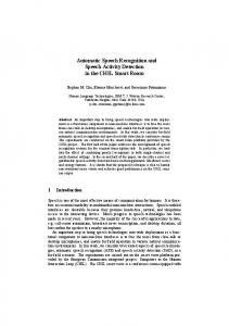
Selecting the token set for language modeling The selection of words as the base units for our language model seems natural. Natural languages seem to be structured so that they contain a small amount of very frequently used words and a huge number of seldom used words. Heaps’ law (Heaps, 1978, page 206) is an empirical law that ties number of unique words V in a text to the number of the words m in the text. V (m) = kmβ (4.1) β and k are parameters that should be empirically set according to the type of the text and the language. The vocabulary growth rates are quite different for different languages depending on the structure of language. Creutz et al. (2007) have calculated the number of unique words in a corpus of a given size for several languages (see Figure 4.1). It seems clear that even using all the unique words appearing in the training set as the vocabulary of the language model, there is no guarantee for all languages that an unseen data set would not contain a significant amount of out-of-vocabulary words. The differences between languages can be explained by their different morphologies. Languages with simple morphology like English can be covered reasonably well by a clearly smaller vocabulary. Finnish, on the other hand, is a highly inflecting language. It also makes use of agglutination and compounding. Thus one sentence in Finnish tends to contain fewer words than a corresponding English sentence, and conversely, one Finnish word contains more information than one English word1 . Consequently, the vocabulary growth rate for Finnish is higher. Let us consider splitting words and using the produced subword units as the basis of our n-gram model. The shorter units we choose, the smaller lexicon we need to achieve a given level of coverage of the language (e.g. if we select a lexicon that contains all characters used for writing the words of the target language, fewer than 100 characters suffice for many languages). A data set split to subword units contains more tokens than the original word-based data. Consequently, the n-gram estimates of any given order are 1 For
example, Finnish word “Ymmärtä-isi-mme-kö-hän” is translated as “would we really understand”
4.1. Examples of subword units
17
2 1.8
ish
n Fin
Unique words [million words]
1.6
oni
Est
1.4
an
1.2 1 0.8
ish
Turk
0.6 0.4
English
0.2 0 0
4
8
12
16 20 24 28 32 Corpus size [million words]
36
40
44
Figure 4.1: Vocabulary growth with respect to the corpus size. Taken with permission from a paper by Creutz et al. (2007).
more accurate, as on average there is more data for each n-gram. On the other hand, the context modeled by an n-gram of a given order is effectively shorter, since on average the subword-based n-gram spans a shorter length of the text than a corresponding wordbased n-gram of the same order. This can be compensated by increasing the order of the n-gram model, but then more n-grams must be estimated.
4.1 Examples of subword units Letters form the smallest symbol set, which can represent the words of the language, thus making the required lexicon very small. On the other hand, in order to model a reasonable amount of n-gram context, very high order n-grams are needed. Also a high number of n-grams is needed, as each letter of a word needs a separate n-gram to model it. For splitting words into syllables, a hand crafted rule set is often needed. For Finnish, an adequate rule set can be created fairly easily. Using the syllables as the lexicon, we can fully cover the Finnish language except for some foreign names and words. From the viewpoint of the application using the speech recognition system, the individual syllables cannot be associated with any meaning. According to standard linguistic theory, morphemes are the minimal meaningful language units; they cannot be divided to smaller meaningful units (Bloomfield, 1935). The systems for splitting words into morphemes are usually fairly complex rule sets, with a lot of embedded expert information, see for example the work by Koskenniemi (1983). The morphemes tend to be somewhat longer than syllables so a reasonable n-gram con-
18
Chapter 4. Selecting the token set for language modeling
text can be covered with a relatively low model order. The fact that the recognition units each have their own meaning can help when developing applications on top of the recognition system. “Left+hand+ed” and “vasen+kät+inen” are examples of a word segmented in morphemes, in English and in Finnish. There are several heuristic methods for automatic segmentation of subword units from words. The advantage of automatic segmentation is that no expert knowledge of the target language is required. Some automatic segmentation systems can be shown to produce units that resemble well-known linguistic constructs like morphemes or syllables.
4.2 Practical issues with subword models Building a speech recognition system using a language model based on subword units requires attention to a few practical points. First, the handling of word breaks merits some consideration. In word-based n-gram models, each language model unit is implicitly assumed to be followed by a word break. For subword units, such an assumption cannot be made. We have decided to add an extra word break token to the vocabulary, which is handled as any other token in the language model. Another way would be to have two versions of each subword token: one that can occur within a word and another that always ends the word. However, this approach would double the size of the lexicon. Acoustically, we have had a few different solutions which all seem to work equally well. The word break can be modeled to have no acoustic counterpart. In this case, the decoder must separately try all hypotheses with and without the word break. We have also modeled the word break acoustically by one HMM state, which seems to work. It should be noted that in continuous speech the word break can generally not really be determined from acoustic information and the decision of whether the word break should be placed or not mostly comes from the language model. Sentence breaks may be treated as usual for word-based models: special symbols marking the start and end of sentence can be used and the n-gram contexts are not modeled past these tokens. For some languages (e.g. Finnish, Estonian, Turkish) mapping from orthography to phonetics is simple. In some Finnish experiments, we prevented any of the algorithms from splitting the words in certain locations: long phonemes (encoded with a double letter, e.g. “aa”) were not split and the letter combination “ng” that maps into one phoneme was not split. When our decoder was improved to model the acoustic context over the borders of the language model units, these restrictions became unnecessary as the context sensitive acoustic models were able to learn the variations. For languages with more complex pronunciation rules, more elaborate schemes may need to be considered. For example, Seneff (2004) presents a system for segmenting words so that the phonetic structure can be reconstructed for English. The decoder design of our system was affected by the decision to use subword models. The first decoder described in Publication 2 of this thesis and the second decoder design by Pylkkönen (2005) both can use high order n-grams in the first recognition pass. Using subword units gives us finer control over pruning the recognition hypotheses, as the language model contributions are taken into account in smaller steps. Instead of
4.3. Related work
19
rescoring each hypothesis when a new word is started, the language model probability is added each time a new subword unit is started. On the other hand, the effective language model lookahead range is reduced, unless higher order models are used for the lookahead. If the language model units allow a word to be built from different combinations of tokens, the different combinations may appear as rival hypothesis. In practice, we have not found this to be a problem, since the worse segmentations seem to be practically always pruned out by the decoder beam pruning.
4.3 Related work Deligne and Bimbot (1995) have presented a method for finding variable length units for language modeling. They build an n-gram model over the found units and demonstrate that the new model outperforms a word-based model. However, it seems that the baseline word model is not well optimized, as the best baseline result was achieved with 2-grams and the results seriously deteriorate when longer context is used. In the follow-up work Deligne and Bimbot (1997) show that their method is capable of finding morpheme-like units from text. They also generalize the method so that it can be used for finding reasonable speech segments from audio data. Geutner et al. (1998) decompose Serbo-Croatian words to stems and suffixes. In their experiments, 3-gram models of the subwords performed clearly worse than the baseline word model. They also tested a two-pass algorithm, where the first recognition pass on a standard word n-gram model is used to produce a word lattice. The stems of the words found in the lattice are searched in the database and the lattice is expanded with all words of the database starting with the stems. This approach gives relative improvement of 16% on the recognition WER. Whittaker and Woodland (2000) use both a hand crafted rule set and heuristic algorithms for splitting words to subword units. They note that the heuristic algorithms seem to be producing morpheme-like units. Using 6-gram subword models interpolated with the baseline 3-gram word model they get relative perplexity improvements around 5% compared with baseline models for both English and Russian. In English speech recognition experiments, the corresponding relative improvement was 2%. They speculate that the improvement could have been larger in Russian speech recognition, but they did not have a Russian recognition system for experiments. Kneissler and Klakow (2001) use a similar setup for Finnish and German experiments. Heuristic algorithms with language expert intervention are used for splitting the words. They make no comparison to wordbased models. Ordelman et al. (2003) split only the less common compound words of Dutch and achieve 2% of relative improvement in WER. Byrne et al. (2001) use morphological rules for decomposing the Czech words into stems and endings. A straight n-gram model over the subword units degrades the recognition performance significantly. Tweaking the n-gram model so that the stems are predicted using the knowledge of previous stems and discarding the endings in between brings the recognition rates back to the level of word n-grams. Kwon and Park (2003) uses a combination of morphological and heuristic rules for Korean speech recognition.
20
Chapter 4. Selecting the token set for language modeling
Szarvas and Furui (2003) use a morphological analyzer for splitting Hungarian words. They also use a morphosyntactic analyzer for deciding which combinations of morphemes are allowed. These are combined into a weighted finite state machine used as the language model. In their experiments, they get 2% relative reduction in WER. Erdo˘gan et al. (2005) use a similar approach for Turkish, except instead of morphemes they use half-words. For 2-gram language models they get a relative improvement of 15%. Increasing the model order reduces the gains, as the morphosyntactic information is already represented in the longer context n-grams. Arısoy et al. (2006) try splitting to syllables, morphemes, stems and endings. They also have a model combining all of the units. They report slight improvements on the recognition letter error rate and no improvements on WER. They used 2-gram models in the recognition experiments. Using higher order models would probably have affected the results. Kirchhoff et al. (2006) compare several different morphologically motivated modes in Arabic speech recognition experiments. They use similar morpheme-based models that are used here (they call these models particle-based), morphological stream models, cluster-based language models and factored language models. In factored language models (Bilmes and Kirchhoff, 2003), each word corresponds to k features or factors. The n-gram model is built over the factor vectors. The main benefit is that the backoff can be specified through a selected subset of the factors. In the experiments, no models give large improvements over the baseline word models. The morphology of Arabic relies on templates, where the consonant template is fixed and determines the basic meaning of the word and the choice of vowels determines the exact meaning of the word. Thus, models that rely on splitting words to smaller units do not match the noncontiguous morphology of Arabic particularly well. Alumäe (2004) also uses morphological analyzer for splitting Estonian. The n-gram morpheme-based model gets a 17% relative improvement over the baseline model in WER. If the morphemes are clustered to 1000 classes and this class model is interpolated with the baseline word model, relative improvement increases to 27%. The thesis of Alumäe (2006) reports extensive experiments with several different models and parameterizations in Estonian. It is noted that relative improvement due to clustering is reduced when training corpus size is increased. Using a factored language model where the word features were augmented with part-of-speech classes and rescoring the n-best list of recognition hypotheses gave 3% relative improvement in WER in the experiments. Further using statistically found word classes as factors did not help. Bisani and Ney (2005) advocate using subword n-gram language models for English. They show that when the recognition data contains a high number of OOV words, the subword model significantly outperforms the word-based model. Even with test data containing a small amount of OOV words, they report improved recognition rates. The subword units try to model single phonemes or graphemes so that the conversions between the two remain simple. Hagen and Pellom (2005) propose using a modified text compression algorithm for finding syllable-like units in an unsupervised manner. Their application, an interactive literacy tutor, should also recognize partially pronounced words. In an English test, their units perform similarly to grammatically generated syllables and outperform statistically
4.4. Introduction to the minimum description length principle
21
generated morpheme-like units. This result is not surprising, since the average length of a syllable-like unit was shorter than the average length of a morpheme-like unit. Thus, the syllable-like units are able to recognize shorter partially uttered words. The research presented in this paragraph is based on the methods presented in Publications 1 and 2, where automatically induced morpheme-like subword units have been shown to work well for Finnish. Hacioglu et al. (2003) compare the baseline word models with morphemes and automatically induced morpheme-like units in Turkish. The morpheme-based model is worse than the baseline word model and the automatically induced subword units achieve 21% relative improvement of WER. Arısoy and Saraçlar (2006) use automatically induced subword units and get 6% relative improvement in WER over the baseline word model for Turkish. Using lattice expansion (as by Geutner et al. (1998)) increases the performance of both word and subword unit based models slightly. Kurimo et al. (2006) test the same approach for Finnish, Estonian and Turkish and get significant gains over word models in all tests. Puurula and Kurimo (2007) compare words with morphemes and automatically induced morpheme-like units in Estonian. Morphemes give relative improvement of 27% in speech recognition tests which was practically equal to the improvement gained by the automatic units (26%). It should be noted that the error rates and relative improvements for the different methods should not be directly compared across different languages. The different morphologies of the languages affect the performances of the methods.
4.4 Introduction to the minimum description length principle Before introducing the automatic splitting method used in the experiments, a mathematical tool used by the method is briefly presented. The minimum description length (MDL) principle states, that the shorter code we can use to describe our data, the better the code models the data (Rissanen, 1989). The MDL algorithms come in many flavors, as discussed by Creutz (2006). Of these, the so-called two-part coding scheme is simple and intuitively fits the problems at hand. In this thesis, all references to MDL refer to this version (also called crude MDL). A problem formulated in the two-part coding scheme can be mapped to an equivalent problem under the maximum a posteriori framework by choosing suitable prior distributions (Creutz, 2006). The two-part coding scheme has been used in the context of language modeling before. Rissanen (1994) outlines how the MDL principle can be used for learning metrical phonology (the organization speech segments into groups of relative prominence). Ristad and Thomas (1995) use the MDL principle for determining the optimal n-gram context lengths in a letter prediction task. In Publications 3 and 4 of this thesis, it is applied to essentially the same problem, that is to determine which n-grams should be included in the language model. Creutz and Lagus (2002) have introduced an MDLbased algorithm for acquiring morpheme-like subword units from a text corpus. We use the subword units generated by their algorithm as the base unit of our n-gram model in Publications 1, 2, 3 and 4. Also Goldsmith (2001, 2006) has presented an MDL-based algorithm for finding morphemes.
22
Chapter 4. Selecting the token set for language modeling
The two-part coding scheme can be explained in the following hypothetical setting: we have two parties and one of the parties wants to transmit data to the other party. Parties are assumed to share some common knowledge, so that they can understand the communication. The data could be transmitted directly, but a more efficient way of sending the data is to transmit first a model describing the data and then the actual data. This assumes that the regularities in the data are captured in the model and the actual data can be described more compactly when this information is taken into account. Thus, we are trying to minimize a two part cost function D consisting of the cost of encoding the model parameters θ and the cost of encoding the data x. The model family λ is assumed to be known by both parties. arg min D = arg min(Dmodel (θ|λ) + Ddata (x|θ, λ)
(4.2)
θ
A problem with the two-part coding scheme is that the optimal cost of encoding the model is not self-evident (this corresponds to choosing the prior distributions in maximum a posteriori estimation). How much prior information should the two communicating parties have about the model family and the model structure? What is the optimal coding for the model given this shared information? In this thesis, the problem is approached in two quite different ways. In the word splitting algorithm (Creutz and Lagus, 2002) the cost function is carefully crafted using combinatorics and elaborate mathematical tools like the universal prior for integers. However, when creating the cost function for encoding an n-gram model (Publications 3 and 4), the cost is directly based on how much memory the model actually takes when loaded into the speech recognition system.
4.5 About the Morfessor algorithm In this work, the Morfessor system by Creutz and Lagus (2002, 2005) is used for automatic word splitting. The method is based on the minimum description length (MDL) principle. The algorithm has few different versions. Here, we describe and use the simplest formulation referred to as the Morfessor baseline method by the original authors. The Morfessor software is available online at http://morfessor.forge.pascalnetwork.org/.
4.5.1 MDL modeling in the Morfessor algorithm Let us define the two parts of the MDL cost function (see Equation 4.2). First, the cost of encoding the model Dmodel can be divided into two parts: the cost of encoding the segment dictionary or lexicon of the model Dmodel (lexicon) and the cost of encoding the probabilities of the segments Dmodel (segment frequencies). The probabilities of the segments will be needed for the second part of the MDL cost function, that is the cost of encoding the training corpus (Equation 4.6). Let us assume that the probability of each character P (α) of the language is known. The code length of each character α is derived from the probability. To spell out a segment w in the lexicon we need to sum over all characters of the segment. Each segment is
4.5. About the Morfessor algorithm
23
assumed to be terminated with a special character marking the end of the segment. Let W be the number of words in the lexicon and length(wi ) the number of characters in the segment i including the end of segment character. The cost of encoding the lexicon is then Dmodel (lexicon) =
W length(w X j) X j=1
− log P (αjk ).
(4.3)
k=1
To encode the segment probabilities, we first send the total number of segments N seen in the training data. N can be encoded using the universal prior for non-negative integers by Rissanen (1989, page 34) U (N ) ≈ log c + log N + log log N + log log log N + . . . ,
(4.4)
�
� N −1 where c is a constant (c ≈ 2.865). As there are ways of choosing W W −1 positive integers that sum up to N , the segment frequencies can be encoded efficiently (Rissanen, 1989, pages 35–37). Dmodel (segment frequencies) ≈ U (N ) + log
�
N −1 W −1
�
(4.5)
As the frequencies of the segments are now encoded, the ML estimates for the segment probabilities can be obtained based on the counts. Having encoded the parameters θ of the segmentation model λ, we can now encode the corpus with the cost of Ddata =
N X
− log P (wi |θ, λ).
(4.6)
i=1
4.5.2 The search for a good model The MDL-based cost function measures how good a given model is. An algorithm for finding the good models is also needed. The Morfessor algorithm uses a greedy search to find the best model. Initially, all words in the training set are put in the lexicon of the model. Each word is then examined separately. All possible ways of splitting the word into two parts are tried. If the best split gives a lower cost than no split, the word is split and the process is recursively applied to the two newly created segments. The algorithm is iterated until convergence. A possible splitting procedure is shown in Figure 4.2. A more formal presentation of the search is given in Publication 2. The described algorithm is used for learning the model. For splitting the actual training corpus of the language model, Viterbi search is used. The Viterbi search can find the segmentations of words not originally used for learning the splitting model. Viterbi search was not used while training the splitting model, since it appears to be more prone to get stuck in local minima of the search space.
24
Chapter 4. Selecting the token set for language modeling
reopen+ed
open+minded
re+open re
open
mind+ed mind
ed
Figure 4.2: Hypothetical splitting trees for English lexicon consisting of two words.
4.5.3 Morfessor as morphological analysis tool For measuring how well the automatic segmentation tool performs for morphological analysis, the segments produced by the algorithm should be compared with the actual morphemes of the given text. Creutz and Lagus (2007) perform experiments comparing the segments of the Morfessor algorithm to those produced by a morphological analysis tool with rule sets built by experts. They also compare their system with another system for learning morphology in an unsupervised manner, the Linguistica system by Goldsmith (2001, 2006). In their tests, all tested versions of the Morfessor algorithm outperform the Linguistica for Finnish. For English, the methods give roughly similar performance. The best algorithms give an F-measure of approximately 0.7 for both languages. They also note that it is better to use the unique word types of the training data instead of using the actual word counts, if morphologically motivated segmentation is desired. The size of the produced segmentation lexicon can be controlled for example by removing the least frequent words from the training set. From now on, we will refer to the subword units produced by the Morfessor algorithm as morphs.
4.6 Experiment I: Subword models vs. word models This experiment was set up to find out, whether using subword n-gram models could significantly improve the speech recognition results. The experiment was originally performed in Publication 1. Both syllable-based and morph-based n-gram models were compared with word-based n-gram models in Finnish perplexity and speech recognition experiments.
4.6.1 Data The text corpus for training the morph segmentation and all the n-gram language models was taken from two sources. Short newswires from the Finnish News Agency (STT) and an early version of the Kielipankki-corpus (CSC, 2007) containing books, magazines and newspapers were used2 . This amounted to 30 million words with 1.6 million unique word forms. For testing, the transcript of the audio data containing 49 000 words was used. 2 Finnish IT center for science has used several names for this corpus during the past years. It has been known as Kielipankki, Suomen kielen tekstipankki, parole-fi corpus and Finnish text collection. Here we will use the original name Kielipankki throughout for clarity.
4.6. Experiment I: Subword models vs. word models
25
The speech data was an audio book read by one speaker. 12 hours were used for training, 8 minutes was used as the development set for tuning the decoder parameters and half an hour was used for testing.
4.6.2 Recognition system setup The reader is referred to Section 2.2 for an overview of our speech recognition system. In this experiment, we used power, mel-cepstral features and their deltas. No feature transformations were used. Triphone models were constructed using the clustering scheme based on the amount of available training data. The acoustic models did not discern between the long and short variants of Finnish phonemes and no explicit duration modeling was used. Deciding which variant to use was left to the language models. The stack decoder was used, so modeling the acoustic context over language model unit boundaries was not possible. When training the acoustic models, the language model units were taken into account: the acoustic context was truncated at the language model unit boundaries. Ignoring the language model unit boundaries during training of the triphones resulted in significantly worse results. During decoding, each hypothesis was created with and without a trailing word boundary regardless of the acoustics, although the acoustic model of silence was forced to produce a word break. Otherwise, the placement of word boundaries was left to the language model.
4.6.3 Language models All language models were 3-gram models with GTK smoothing. The models were trained with the CMU-Cambridge statistical language modeling toolkit by Clarkson and Rosenfeld (1997). For the word-based model, the 64 000 most common words of the training set were used. For subword models, the word splitting was prevented in the middle of letters that map to one phoneme. The lexicon of our syllable-based n-gram model contained 37 000 unique units. This high number is due to the restriction on possible splitting points and due to the fact that Finnish rules were also used to segment foreign words. The early version of the Morfessor algorithm (Creutz and Lagus, 2002) used for segmenting the words did not take into account the coding cost of the morph frequencies (Equation 4.5). In practice, omitting this term in the cost function does not affect the segmentation much. The algorithm produced 300 000 unique morphs from our training set. This number was reduced to 65 000 different morphs by pruning the least frequently seen ones from the lexicon. The training data was resegmented using the pruned lexicon resulting in effective 0% OOV rate.
26
Chapter 4. Selecting the token set for language modeling
Table 4.1: Perplexity results.
lexical unit word syllable morph
number of units 64000 36850 64684
OOV words 20.2% 0.02% 0.00%
3-gram hits 18.2% 98.9% 77.6%
word perplexity 4 300 65 800 28 500
Table 4.2: Speech recognition results. LER stands for letter error rate.
lexical unit word syllable morph
WER 56.4% 43.9% 31.7%
LER 13.8% 10.9% 7.3%
4.6.4 Experimental results The models were first tested on the transcript of the audio data. The results for the 3-gram models are given in Table 4.1. Although the lowest perplexity is by the wordbased model, the low value is achieved by not modeling every fifth word at all (20% OOV rate). The other models have significantly higher perplexity, but model practically all words, also the rarest ones. This comparison does not take into account that if the n-gram order is chosen to be the same for all of the models, the models based on longer units can model longer contexts. This can be seen, when we examine the percentage of the highest order models used for modeling the test data. Word-based models only need the highest order context occasionally, whereas the syllable models rely on the highest order models practically always. Increasing the n-gram order would probably not benefit the word-based model nearly as much as it would improve the syllable-based model. Corresponding speech recognition results are given in Table 4.2. The word-based model does not achieve good recognition scores due to the high OOV rate. The syllable-based model still suffers from the shortness of the modeled context. The morph-based model appears to give the best results. Note that the decoder cannot model acoustic contexts over the language model unit boundary, but the inter-unit dependencies are modeled. Thus speech recognition experiment is slightly biased in favor of the models based on longer units, since using them results in fewer language model unit boundaries. Based on this experiment, it was decided to conduct further research on the use of subword units for modeling languages like Finnish.
4.7 Experiment II: Morphs in n-gram models This experiment was conducted to show that morph-based models are at least as good as models based on words or morphemes generated by grammatical rules. This experiment was originally conducted in Publication 2.
4.7. Experiment II: Morphs in n-gram models
27
4.7.1 Data The data used on the experiments was mostly the same as in Experiment I (Chapter 4.6.1). As slightly newer version of Kielipankki corpus was used, the combined word count of the Kielipankki corpus and STT newswires was now 40 million words. The text data was converted to corresponding phonetic transcript.3 It is easy to transform this transcript back to text for Finnish words, as the corresponding rules are simple. For foreign names, the mapping from phonemes to text is ambiguous. The language models were trained on the phonetic transcripts. We used the same audio book as in the first experiment with 20 minutes of data set aside for development and 30 minutes for evaluation. This task is here referred to as the book task. Furthermore, we used 5 hours of news read by one speaker. 3.5 hours of data were used for training, 30 minutes for development and 49 minutes for evaluation. This is referred to as the news task. In addition to training acoustic models, the reference transcripts of the training portions of the audio data was used for evaluation of the language models.
4.7.2 Recognition system setup Compared with the recognition system used in the previous experiment (see Section 4.6.2), some changes were made. We still use the older decoder design, but now we decided to use monophones, so that models with longer units would not gain advantage on the recognition experiments. The phoneme state durations were modeled and the emission probability distributions for the long and short phonemes were modeled separately. A maximum likelihood linear feature transform was applied as described in Section 2.2.
4.7.3 Language models We constructed three different word-based models for our baseline models. First, we trained a model using 410 000 most common words of the training set. The rest of the words were tagged with the “unknown word” symbol. Second, we trained a similar model, except that all unknown words were split to phonemes and the n-gram model was thus using a mixture of words and phonemes, resulting in 0% OOV rate. Two variants of phonemes were used, a phoneme at a word boundary and a regular phoneme. This provides unambiguous word boundaries. Third, a word model using 69 000 most common words with unknown words split to phonemes was trained. We also trained an n-gram model based on morphemes generated by a morphological analyzer4 utilizing a sophisticated rule set based on the two-level morphology of Koskenniemi (1983). The analysis produced 79 000 different morphemes. Finally, the Morfessor algorithm using the full cost function presented in Section 4.5.1 was used. Using the word types found in the training set as the input for Morfessor, we obtained 66 000 different morphs. Removing the word forms seen fewer than three times 3 We are grateful to Nicholas Volk from Helsinki University for kindly providing the software. http://www.ling.helsinki.fi/suopuhe/lavennin/. 4 Licensed from Lingsoft, Inc.: http://www.lingsoft.fi
28
Chapter 4. Selecting the token set for language modeling
Book 19
News 19
Words 69k Words 410k Grammatical 79k Statistical 66k Statistical 26k
18
18
17 Entropy (bits)
17 Entropy (bits)
Words 69k Words 410k Grammatical 79k Statistical 66k Statistical 26k
16
15
16
15
14
14
13
13
0
100
200
300 400 Size (MB)
500
600
0
100
200
300 400 Size (MB)
500
600
Figure 4.3: The cross-entropy of the different models on the test data versus the corresponding model sizes. The six points along each curve are the orders 2–7 of the n-gram models.
in the corpus resulted in 26 000 different morphs. Both models were used in the tests. Running the Morfessor algorithm on the word counts of the training data, where words seen fewer than 20 times were removed, results in 35 000 morphs. It seems like these morphs did not correspond as well to the morphological segmentation as the morphs generated by the other means, so this splitting was not further tested. We created n-gram models of orders from 2 to 7 using the SRILM toolkit with the default cutoffs (Stolcke, 2002). The models were smoothed with modified KN smoothing.
4.7.4 Experimental results The results of the cross-entropy experiments with the phonemic transcripts of the text data are given in Figure 4.3. We did not run the experiments on the word model containing OOV words, since that comparison would have been meaningless (7.3% OOV rate for the book task and 5.0% for the news task). It is clear from the results that the subword units are clearly more efficient with smaller models, but for larger models the performances seem roughly equal. We can observe one weakness of the rule-based morphological analysis: the rule set does not contain rules for segmenting foreign words or names. The statistical approach can produce some kind of segmentation for these words and seems to get better results in the news task, where the foreign names and words are more frequent.
4.7. Experiment II: Morphs in n-gram models
29
Book 12
12
Words 69k Words−OOV 410k Words 410k Grammatical 79k Statistical 26k Statistical 66k 3
10 9
10
4 8 5 7
34 5 3
6
4
5
3
5
3
4
4
0
100
9 8 3
7
5
200 300 Model size (MB)
4
3 4
6 3
5
5
4
Words 69k Grammatical 79k Words 410k Words−OOV 410k Statistical 26k Statistical 66k
11
Phoneme error (%)
11
Phoneme error (%)
News
4
5 5 3 4 5 34 5 5
4
400
0
100
200 300 Model size (MB)
400
Figure 4.4: Phoneme error rates and model sizes for different n-gram orders.
The speech recognition experiments were run for the model orders 3, 4 and 5 and the results are shown in Figure 4.4. We have chosen to report the phoneme error rates, as this measure is more sensitive to small errors. Also, the language models output phonetic transcription so this error measure was the most straightforward to evaluate. The phoneme error rate correlates very well with the letter error rate as there is a oneto-one mapping between the phonetic and written form of the Finnish words. In the book task, the models based on morpheme-like units give clearly better results than the word-based models. The results on the news task are surprisingly different. It seems like the word-based models are more sensitive to the differences in the training and testing set domain: in the news task, the word-based models are much closer to the morph-based models. This improvement of the word models is probably accounted by the fact that the vocabulary of the word-based models cover the news set better and the models do not need to use the phoneme-based part of the n-grams that much. The phoneme-based n-grams are not a big problem in the evaluation of text entropy, but they seem to make the hypothesis search in the decoder harder. On the other hand, the rule-based morpheme models perform significantly worse in the news task. The reason seems to be that the task contains a higher number of foreign words, for which no rules have been written. For these words, the rule-based model has to fall back on phoneme-by-phoneme decomposition. The statistical significance of the results was tested with the Wilcoxon signed-rank test (see Publication 2 for details). The most important results were that the models based on morpheme-like units were significantly better in the book task and that the morphs
30
Chapter 4. Selecting the token set for language modeling
were significantly better than the other models in the news task. These would seem to be the interesting and practically significant differences, as well.
4.8 Concluding remarks In this chapter, the problem of modeling a highly inflecting language using subwordbased n-gram models was examined. Some problems with the baseline word-based approach were observed. A high OOV rate for unseen data was reported, even for models with a very large vocabulary. It seems that the OOV words also reduce the model performance for other words, as the context of the words is recognized incorrectly. It has been demonstrated that the subword-based n-gram models work well for Finnish. Of the tested models, the ones based on automatically induced morphs seem to work best in our experiments. The morphemes generated by a rule set work well, when the data is well covered by the rules. However, the automatic method can be applied to new languages without expert knowledge and seems to give superior results. The morphs have been used for Turkish and Estonian speech recognition systems as discussed in Section 4.3 and seem to work well for these languages also. The n-grams to be included in the model were chosen simply by taking all n-grams of the training set that were at most as long as the maximum model order and then removing the most infrequently seen n-grams. It seems likely that especially the models based on short subword units would benefit from a more elaborate method for choosing the ngrams to be included. Preliminary experiments using the methods presented in the next chapter indicate that the syllable-based models are almost as good as the morph-based models, when the n-grams of the model are selected with care. Letter-based models however do not seem to give that good performance with respect to the model size.
31
Chapter 5
Selecting the set of n-grams for the model Let us examine an interpolated n-gram model, in which all n-grams from the training corpus up to a given order are included. It is obvious that not all n-grams of the model give equal contributions to the predictive power of the model. Let us start from the 2-gram probability estimate with the known one-word history “Tarja”. Increasing the model to 3-grams with the words “president Tarja” should improve the modeling accuracy considerably.1 Further increasing the modeled context to “with president Tarja” on the other hand does not bring much additional information to the model and the corresponding n-gram could be removed. The modeling accuracy of n-gram models is usually limited by the amount of memory available. Thus, reducing the size of the model without degrading the predictive power of the model is important. The methods for size reduction can be roughly divided in three categories: lossless compression of the model, compression by quantization and compression by choosing only the most relevant n-grams for the model. In this chapter, the last issue is chosen for examination. The interaction between pruning and quantization has been studied for example by Whittaker and Raj (2001a).
5.1 Related work The simplest way of choosing the n-grams to be included in the language model is to include all n-grams found in the training set up to the desired highest order. This so-called full model can be reduced in size by two complementary methods: frequencybased pruning removes the n-grams that have been seen so few times that their estimates are considered inaccurate. Likelihood-based pruning removes the n-grams that do not increase the modeling power significantly. When dealing with large data sets, it may be impossible to construct a full model which 1 The
current president of Finland is Tarja Halonen.
32
Chapter 5. Selecting the set of n-grams for the model
includes all the relevant n-grams due to memory constraints. Growing methods use greedy search algorithms for adding the useful n-grams to the model and discarding the less useful ones. This allows to add also the relevant high-order n-grams to the model. Also the grown models can often be refined by pruning the resulting model. In this section, we will examine work related to these issues.
5.1.1 Pruning n-gram models The simplest frequency-based pruning method is the count cutoff method. The n-grams seen fewer than mn times are removed from the model, where the cutoff limit is usually specified separately for each model order n. A related idea is to remove the n-grams hw, for which the context h has been seen fewer than m|h| times. Seymore and Rosenfeld (1996) have presented a simple likelihood-based pruning method called weighted difference pruning (WDP) which operates as follows. An n-gram is chosen from the model. The log-likelihood of the n-gram given by the current model is compared with the log-likelihood given by a model, where the current n-gram has been removed. The difference is weighted by a Good-Turing smoothed estimate of the frequency of the n-gram. If the weighted likelihood does not exceed a given threshold, the n-gram is removed from the model. The procedure is repeated once for all n-grams in the model. In the experiments, the model size reduction by decreasing the amount of training data is compared with model size reduction by WDP and the conclusion is that WDP gives better results. WDP is also compared with count cutoffs: for the WDP model, a small count cutoff is applied first and then the pruning is performed. When this is compared with a model of equal size, where more severe cutoffs have been used, the WDP model consistently gets better perplexities. No comparison included a WDP model with no count cutoffs. The WDP criterion does not take into account that removing an n-gram hw from the model also changes the probabilities of other n-grams. Since the backoff coefficient κ(h) is modified, estimates for all n-grams that utilize the back-off coefficient are modified. Stolcke (1998) presents the entropy-based pruning (EP) method and shows how all changes in the probability can be efficiently estimated. In the experiments, EP slightly outperforms WDP. A more detailed description of EP is given in Section 5.2.1. Kneser (1996) has also presented a likelihood-based pruning method called Kneser pruning (KP). In KP, an AD model is used for determining the cost of removing ngrams from the model. The cost is determined similarly as for WDP. When the set of n-grams to be included in the model has been decided, the model is estimated using similar principles as in KN smoothing. KP is described in detail in Section 5.2.2. Goodman and Gao (2000) show that count cutoffs work well when only slight pruning is required. However, for more severe pruning both WDP and EP are shown to work better. Also the experimental results by Bonafonte and Mariño (1996) with a very small training set show that the combining frequency-based and likelihood-based methods gives the best results. Niesler and Woodland (1999) experiment with pruning cluster-based ngram models. They observe that their likelihood-based pruning criterion consistently outperforms the combination of count and context cutoffs.
5.1. Related work
33
In this work, the likelihood-based methods are further studied. It will be shown that the existing pruning methods do now work well with the state-of-the-art KN smoothing. A new pruning method for KN smoothed models called revised Kneser pruning (RKP) is presented and the method is discussed in detail in Section 5.2.3. The method uses a few different approximations than the other methods and it is shown in the experiments (Section 5.3) that the method gives excellent results.
5.1.2 Growing n-gram models Ristad and Thomas (1995) present a MDL-based method for growing an n-gram model. When deciding whether an n-gram should be inserted into the current model, the benefit of the increased modeling accuracy is weighted against the amount of bits needed for storing the n-gram. The greedy search tries to insert all n-grams hw for which the prefix h already exist in the model. In the experiments, a text containing 900 000 letters is used for training letter-based n-gram models. They report significant improvements over the baseline full n-gram model. However, it seems that the baseline model is not very good as the performance of the model degrades rapidly when higher order n-grams are used. Also Ron et al. (1996) have presented a similar growing algorithm, which is formulated in the framework of probabilistic finite automata. The n-gram selection is based on a combination of frequency and likelihood-based criteria. Niesler and Woodland (1999) present a word clustering algorithm. The cluster n-gram model is grown by an algorithm, where new n-grams are added by a greedy algorithm similar to the one by Ristad and Thomas (1995). The cost criterion is based on leave-one-out cross validation. Siu and Ostendorf (2000) present the n-gram model in a tree structure. They show, how operations for modifying the tree correspond to pruning the n-gram model, word skipping and context-dependent word clustering. They also show how the tree can be grown. In their experiments, the most significant improvements were gained through finding the optimal model context length. The tree is grown one distribution at a time and contrary to the other methods, the search algorithm proceeds by growing the ngrams towards the past. A new algorithm for growing KN smoothed n-gram models called Kneser-Ney growing (KNG) is described in Section 5.2.5. The growing algorithm is similar to the one by Niesler and Woodland (1999). The selection criteria is based on the MDL principle. Whereas Ristad and Thomas (1995) use an elaborate theoretical MDL cost, a simpler and more practically oriented MDL cost function is used in KNG. In the experiments described in Section 5.3, the growing method is shown to improve the results obtained by RKP.
5.1.3 Other related work There are other ways for controlling the context modeled by the n-gram model. Several adjacent words can be merged and used as one token in the language model, as shown for example in the paper about word clustering by Yamamoto et al. (2003). Deligne and Bimbot (1997) have also studied combining several observations into one underlying
34
Chapter 5. Selecting the set of n-grams for the model
token. The related idea of splitting words into subword units was studied in Chapter 4 of this thesis. Seneviratne and Young (2005) present a language model with a hidden vector state. The state of the model is a simple stack of a push down automaton. Based on the state, the next word can be predicted. In practice, the probability estimation is decomposed so that the model can choose which words of the history the estimate for the probability of the next word is based on. In the experiments, a cluster-based model with around 100 clusters is estimated using both n-gram and hidden vector state methods. For this restricted task, the hidden vector state models are shown to give consistent improvements in perplexity, around 10%. Virpioja and Kurimo (2006) present a method for growing variable order n-gram models, where the context can be clustered. In experiments, their method is compared with the earlier version of KNG (Publication 3 of this thesis) with a fairly small training set of around 10 million words. In the experiments the clustered models give somewhat better results. Publication 4 describes, how using a more efficient pruning algorithm can improve the results. Virpioja has performed preliminary experiments and the results indicate that applying similar changes to their algorithm provides comparable improvements. It is possible to select only some word positions of the given context that will be taken into account. These so-called skip n-gram models have been introduced in the context of both traditional n-grams (Huang et al., 1993; Martin et al., 1999) and maximum entropy models (Rosenfeld, 1994). The extensive tests of Goodman (2001) also included skip n-gram models. His conclusion is that skip n-grams are reasonable for small and intermediate amounts of data, especially if high order n-grams cannot be used for some reason. One motivation for using these methods is to avoid adding a full new order to the n-gram model. The pruning and growing methods presented in this chapter produce a similar effect.
5.2 Algorithms for pruning and growing n-gram models Let us start by defining a few terms. A non-leaf n-gram hw of a model is an n-gram, which is a prefix of some other n-gram hwv found in the model. Correspondingly, a leaf n-gram hw is an n-gram, which is not a prefix to any other n-gram. This terminology stems from the presentation of the language model as an n-gram prefix tree. The mathematical notations and the smoothing methods relevant to this section were presented in Chapter 3.
5.2. Algorithms for pruning and growing n-gram models
35
5.2.1 Entropy-based pruning (EP) EP for backoff models was presented by Stolcke (1998). The cost d of removing n-gram hw form the model M is defined as d(hw) =
X
PM (hv) log
v
PM (v|h) PM ′ (v|h)
(5.1)
PM denotes the probability estimate of the original model and PM ′ is the estimate of a model, where the n-gram hw has been removed. The summation over words v reflects the fact that the probability estimates of other n-grams change as well when the backoff weights are recalculated for the pruned model. This change can be efficiently computed. When the cost of removal has been calculated for all n-grams of the model, the n-grams for which the cost does not exceed a given threshold are removed from the model. EP has some approximations. The pruning of one n-gram is assumed to be independent of the pruning of any other n-gram. It is assumed that PM (c|b) is a good estimate for PM (c|ab). This is a valid approximation when the smoothing of the model does not optimize the lower order probability distributions based on higher order distributions (e.g. for AD and GTK). The same approximation is used for the weighting PM (hv). Also, it is assumed that the weighting can be approximated from the n-grams of the model. P (abc) ≈ PM (a)PM (b|a)PM (c|ab)
(5.2)
EP has the advantage that besides the original model, no additional information is required for performing the pruning. Some other methods require that the counts of the n-grams from the training data should be also known. On the other hand, some of the approximations of EP do not work well with KN smoothing.
5.2.2 Kneser pruning (KP) In KP (Kneser, 1996), an auxiliary model using AD is built first. Using the AD model, the set of n-grams to be removed from the model is determined. The cost of removing a leaf n-gram d1 (hw) is defined as d1 (hw) = P (hw) log
P (w|h) ˆ γM (h)P (w|h)
.
(5.3)
The cost of removing a non-leaf node d2 (hw) is the average of the costs of removing all the n-grams, which have hw as prefix. When all the n-grams of the model have been tested for removal, a new model is built using only the remaining n-grams. The new model tries to preserve the marginal distributions (Equation 3.11) similarly to KN smoothing. Appendix A.2 shows the associated
36
Chapter 5. Selecting the set of n-grams for the model
approximations. The resulting probability estimate is2 ) ( X X C(vhw) + D|hw| 1 − D|h| max 0, vhw∈λ
vhw ∈λ /
P (w|h) =
P
w′
X
′
C(vhw ) + D|hw′ |
vhw ′ ∈λ /
X
vhw ′ ∈λ
1
!
ˆ (5.4) +γ(h)P (w|h),
where the notation vhw ∈ λ refers to the n-grams included in the model λ and vhw ∈ /λ to the n-grams not in the model. The value of the the interpolation coefficient γ can be easily solved. The method uses several approximations. The removal of an n-gram is assumed to only change the probability of that n-gram and the changes due to changing interpolation coefficients γ are ignored. The selection criterion is based on a different kind of model than the final model. Like in EP, the removal of an n-gram is assumed to be independent of the removal of any other n-gram. Also like EP, for the purpose of weighting the cost criterion the model probability P (c|ab) is assumed to be a good estimate for P (c|b). Since the model selection is made using an AD model, this estimate is reasonable. In preliminary experiments we noticed that different approximations have a significant impact on the performance of the method.
5.2.3 Revised Kneser pruning (RKP) In this section, an algorithm for pruning KN smoothed n-gram models is presented. The algorithm is related to both KP and EP, but some approximations are different. The RKP does not assume that the pruning of different n-grams is independent. Instead, an n-gram is removed immediately after the pruning decision has been made, resulting in a simple greedy search for the best model. For the pruning criterion, the WDP cost criterion is used, except instead of using the Good-Turing discounted n-gram count for the weighting, we use the n-gram count in the training set. This is simpler, but probably slightly less accurate. When an n-gram is pruned, the lower order distributions of the model are modified. The modification relies on a simple observation: in the original KN smoothing for full models (see Equation 3.12), the probability estimates for the highest order n-grams (leaf n-grams) are based on the number of n-grams in the training set. For the non-leaf ngrams, the estimates are based on the number of different words that can precede the n-gram. It turns out that when an n-gram is removed from the model, the model can be easily modified to reflect this behavior. Let us initialize the variables with the values of a full KN smoothed model.3 Additionally for each pruned n-gram hw, the sum of pruned counts L(h) for the prefix h 2 The original paper presents the estimate for a backoff model (Kneser, 1996, Equation 9) and there are parentheses missing around N (v, hk , w) − d in the numerator and denominator. Despite the different appearances, the equations are otherwise equivalent. 3 C(hw) and S(h) were defined in Section 3.1.1. D ′ |h| was defined in Section 3.1.2 and C (hw) was defined in Section 3.1.3.
5.2. Algorithms for pruning and growing n-gram models
37
P RUNE O RDER (k, ǫ) 1 for {hw : |hw| = k ∧ C ′ (hw) > 0} do 2 logprob0 ← C(hw) log2 PKN (w|h) 3 P RUNE G RAM (hw) 4 logprob1 ← C(hw) log2 PKN (w|h) 5 if logprob1 < logprob0 − ǫ 6 undo previous P RUNE G RAM P RUNE G RAM (hw) 1 L(h) ← L(h) + C ′ (hw) ˆ >0 2 if C ′ (hw) ′ ˆ ˆ + C ′ (hw) − 1 3 C (hw) ← C ′ (hw) ˆ ˆ 4 S(h) ← S(h) + C ′ (hw) − 1 ′ 5 C (hw) ← 0 Figure 5.1: The pruning algorithm. k is the order to be pruned and ǫ is the pruning threshold. Note that lines 3 and 6 in P RUNE O RDER modify the counts C ′ (·), which also alters the estimate PKN (w|h). P RUNE O RDER is called for each order of the model starting from the highest order.
is updated. The RKP algorithm is shown in Figure 5.1. The algorithm is allowed to prune non-leaf nodes even though this may not be theoretically justified. Preliminary experiments indicate that pruning the non-leaf nodes improves the performance of the method. The probability estimates of the model are similar as for KN smoothing (Equation 3.8), but now the pruned probability mass has to be taken into account. P (w|h) =
max{0, C ′ (hw) − D|h| } ˆ + γ(h)P (w|h) S(h) + L(h)
The interpolation coefficient γ is {v : C ′ (hv) > 0} D|h| + L(h) . γ(h) = S(h) + L(h)
(5.5)
(5.6)
For efficiency, a separate variable for {v : C ′ (hv) > 0} can also be maintained. Also, C(hw) may be replaced by C ′ (hw) in lines 2 and 4 of P RUNE O RDER for a slightly lower memory consumption and slightly faster computation. In preliminary experiments, this did not affect the performance of the produced models.
5.2.4 Comparison of the approximations of EP, KP and RKP EP and KP assume that pruning an n-gram is independent of the other pruning operations while in RKP, the model is modified immediately after the pruning decision has been made. This results in a simple greedy search for the best model. Also, KP uses different model to decide, which n-grams to remove, than the final KN smoothed model. The selected set of n-grams is probably quite different from the set that would be chosen
38
Chapter 5. Selecting the set of n-grams for the model
using the correct model. After the set of n-grams to be pruned has been decided, KP and RKP are almost equivalent. Indeed, the estimates of the RKP model (Equations 5.5 and 5.6) are identical to the estimates of the KP model (Equation 5.4) except that KP term D|hw| is approximated to be 1. The approximation allows for a more efficient search, when the discount parameters are optimized on held-out data after pruning. Also, in the given form RKP can easily be generalized to use three discounts, similarly to modified KN smoothing. The main difference between KP and RKP is in the selection of the n-grams to be pruned. As will be seen in the experiments (Section 5.3), RKP seems to give clearly superior results. EP takes into account, how the probability of all n-grams change when the current ngram is removed, whereas KP and RKP only calculate the difference for the current n-gram. In practice, the difference due to this should be small: WDP and EP perform almost equally well (Stolcke, 1998). On the other hand, EP does not modify the lower order distributions. Also, the weighting of the difference of the log likelihoods is based on an approximation that does not hold well for KN smoothed models (Equation 5.2). In the experiments (Section 5.3), RKP is shown to outperform EP for KN smoothed models.
5.2.5 Kneser-Ney growing (KNG) It is also possible to construct a language model by starting from an empty (or a 1-gram) model and searching for the n-grams that should be added to the model. In this section, a growing algorithm based on the same principles as RKP is presented. Let us initialize the model to a 1-gram KN smoothed model. As all possible combinations of n-grams cannot be tried, greedy search is used. For each n-gram hw in the model, the algorithm tries adding all n-grams hwv in the training set to the model. As the n-grams are added, the model is modified according to the following principle: leaf nodes should utilize the counts from the training data as the basis for the probability estimates, whereas non-leaf nodes should use the number of words preceding the n-gram in the training data. Figure 5.2 describes the growing algorithm in detail. The factor δ is used for controlling the relative importance of the modeling accuracy with respect to the model size. Increasing δ decreases the size of the resulting model. The probability estimates of the model are the same as for RKP (Equations 5.5 and 5.6). The purpose of the pruning algorithms presented earlier is to reduce the model size. The presented algorithms implicitly assume that all n-grams have equal impact on the model size. In KNG, we have chosen to use an explicit cost function for modeling the cost of storing the n-gram. The cost function is defined in the MDL framework. The derivation of the cost function is presented in Appendix A.3. The resulting cost function consists of two parts: the well-known weighted difference of log likelihood and the cost of encoding the n-gram in the model, which is given below. ∆Cost = α(Nnew − Nold ) + Nnew log2 Nnew − Nold log2 Nold
(5.7)
N is the number of n-grams in the model. The constant α is related to the number of bits used for storing the probability estimates. A similar cost function can also be used for RKP. The resulting cost function is quite close to the implicit cost used in the
5.2. Algorithms for pruning and growing n-gram models
G ROW O RDER (k, δ) ′ 1 for {h : |h| = k − 1′ ∧ C (h) > 0} do 2 size0 ← {g : C (g) > 0} 3 logprob0 ← 0 4 for w : C(hw) > 0 do 5 logprob0 ← logprob0 + C(hw) log2 PKN (w|h) 6 for w : C(hw) > 0 do 7 A DD G RAM (hw) 8 size1 ← |{g : C ′ (g) > 0}| 9 logprob1 ← 0 10 for w : C(hw) > 0 do 11 logprob1 ← logprob1 + C(hw) log2 PKN (w|h) 12 logscost = size1 log2 (size1 ) − size0 log2 (size0 ) 13 sizecost ← (size1 − size0 )α + logscost 14 if logprob1 − logprob0 − δ · sizecost ≤ 0 15 undo previous A DD G RAM(hw) for each w 16 re-estimate all discount parameters Di A DD G RAM (hw) 1 C ′ (hw) ← C(hw) 2 S(h) ← S(h) + C(hw) ˆ >0 3 if C ′ (hw) ′ ˆ ˆ − C(hw) + 1 4 C (hw) ← C ′ (hw) ˆ ˆ 5 S(h) ← S(h) − C(hw) + 1 Figure 5.2: The growing algorithm. k is the order to be grown and δ controls the relative importance of the model compactness in comparison to the model accuracy.
39
40
Chapter 5. Selecting the set of n-grams for the model
pruning algorithms, where ∆Cost = α(Nnew − Nold ). A theoretically more accurate cost function, like the one used by Ristad and Thomas (1995) can be defined. Since we are trying to optimize the performance of the model with respect to the model size in a real speech recognition system, the proposed cost function should give better values. Since KNG grows the model one distribution at time, there will still be individual ngrams in the model that do not contribute much to the overall modeling accuracy. These can be pruned with RKP. Also, to improve the search for the best model, it would be possible to make the search less greedy and alternate between the growing and pruning phases. The resulting search algorithm would be akin to simulated annealing and could possibly avoid some local minima. However, this would significantly increase the computational burden of the algorithm.
5.3 Experiment III: Comparison of pruning and growing algorithms In this section, the EP, KP, RKP and KNG algorithms are compared. The experiment was originally presented in Publication 4.
5.3.1 Data For training the Finnish language models, we used 150 million words from the Kielipankki corpus (CSC, 2007). Simple preprocessing for cleaning up the data and spelling out any number sequences was performed. Then the data was split to 8428 unique morphs using the Morfessor algorithm (Creutz and Lagus, 2005) with no restrictions to where a word could be split. This resulted in corpus of 460 million morphs. For the methods that require a held-out data set, 110 000 morphs were set aside. 510 000 morphs were left to the test set. The audio data for the Finnish speech recognition tests was taken from the SPEECON corpus (Iskra et al., 2002). Only adult speakers in clean recording conditions were used. The training set consisted of 26 hours of material by 207 speakers. The development set was 1 hour of material by 20 different speakers and the evaluation set 1.5 hours by 31 new speakers. Only full sentences without mispronunciations were used in the development and evaluation sets. The English text corpus was taken from the second edition of the English LDC Gigaword corpus (Graff et al., 2005). 930 million words from the New York Times were used. The last segments were excluded from the training set: 200 000 words for the development set (if needed by the method) and 2 million words for the test set. 50 000 most common words were modeled and the rest were mapped to an unknown word token.
5.3. Experiment III: Comparison of pruning and growing algorithms
41
5.3.2 Recognition system setup The reader is referred to Section 2.2 for an overview of our speech recognition system. In this experiment, power and mel-cepstral features with deltas and delta-deltas were used. Maximum likelihood linear feature transform and cepstral mean subtraction were used. Triphones were clustered using the decision-tree-based algorithm. No special processing was made to convert the text to phonemes and the system relied on the triphone models (actually triletter models) to find the correct pronunciation for each letter based on the context. For modeling the context of triphones, short silences between words were removed and the adjacent letters were used instead. The word boundaries were modeled by a one-state model of a short silence. The simple postprocessing approach was used for modeling the phoneme durations. For this experiment, the new decoder was used.
5.3.3 Language models For the Finnish experiments, full 5-gram models were constructed using KN smoothing, modified KN smoothing and GTK smoothing. The SRILM toolkit (Stolcke, 2002) was used to perform EP on the modified KN smoothed and GTK smoothed models. KP was used for KN smoothed models. RKP was used on the modified KN smoothed model. KNG was used to grow a model to similar size as the full unpruned 5-gram model and the resulting model was pruned with RKP. For the English experiments, full 4-gram models were built using KN smoothing and modified KN smoothing. A KNG model was grown to the largest size that was practical with our implementation. KP was used for the KN smoothed model. RKP was used for the modified KN smoothed model and the KNG model. Also, GTK and KN smoothed 4-gram models, where all 3-grams seen once and all 4-grams seen 3 or fewer times were removed, were built. Both models were pruned by EP. The cutoffs were used to reduce the memory consumption of the SRILM tools so that the models could be estimated and pruned.
5.3.4 Results and discussion The results of the Finnish and English cross-entropy experiments are shown in Figures 5.3 and 5.4. The reader should remember that the cross-entropies (or perplexities) are not comparable across languages. The sentence cross-entropy for the best model of each language was around 160 bits. An English sentence contained on average 20 words and a Finnish sentence 11 words. This means that the Finnish cross-entropies are almost double the English cross-entropies and the Finnish perplexities are almost the English perplexities squared. A Finnish sentence had on average 34 morphs (word break tokens included). The results confirm that KN smoothing outperforms GTK smoothing for full models. The differences between KN smoothing and modified KN smoothing are small. It can be seen that the older pruning methods (EP, KP) do not work well for KN smoothing.
42
Chapter 5. Selecting the set of n-grams for the model
5g EP (KN) 5g KP 5g EP (GT) 5g RKP KNG
Cross−entropy (bits / word)
15.5
15
46341
32768 Word perplexity
small 14.5
23170
14
16384
medium large
full
13.5
11585
13
8192 6
7
10
8
10 10 Model size (number of n−grams)
Figure 5.3: Cross-entropy results on the Finnish text corpus. Note that the reported cross-entropy and perplexity values are normalized per word.
Cross−entropy (bits / word)
8.1 small 8
294 274 256
7.9
239
7.8
223
7.7
Word perplexity
4g EP+cutoff (KN) 4g KP 4g EP+cutoff (GT) 4g RKP KNG
8.2
208
medium
7.6
194 large
7.5
full 181
7
8
10 10 Model size (number of n−grams)
Figure 5.4: Cross-entropy results on the English text corpus.
5.3. Experiment III: Comparison of pruning and growing algorithms
small 60 n−grams (%)
medium 5g EP (KN) 5g KP 5g EP (GT) 5g RKP KNG
50 40 30
70
50 40 30
20
20
10
10
0
1
5 order
5g EP (KN) 5g KP 5g EP (GT) 5g RKP KNG
60 n−grams (%)
70
0
10
1
large
n−grams (%)
60 50 40 30
70
50 40 30 20
10
10 1
5 order
10
10
all 5g full KNG
60
20
0
5 order full
5g EP (KN) 5g KP 5g EP (GT) 5g RKP KNG
n−grams (%)
70
43
0
1
5 order
10
Figure 5.5: Distribution of n-grams of different orders for Finnish. Orders up to 10 are shown. The highest order in the KNG model was 16.
Taking higher order counts into consideration with the KNG algorithm can clearly benefit the model. The n-gram distribution over the n-gram order for the models is drawn in Figure 5.5. The distributions become more similar as more pruning is applied. Figure 5.6 shows the relative portion of n-gram orders utilized when evaluating the test set. From the figures it can be seen that both KP models and EP models with KN smoothing produce notably different distributions compared with the other methods. These two methods were also the worst performers. It can also be seen that the grown model utilizes a significant amount of the high order n-grams which were not included in the other models. In the English cross-entropy experiments we see that the 4-gram models pruned only with count cutoffs work surprisingly well. The reason for using the cutoffs was to bring down the memory consumption so that SRILM tools could be used. However, the results seems to confirm that using slight cutoffs is beneficial. Later preliminary experiments showed that cutoffs seem to give similar benefits for the RKP and KNG algorithms. Pruning the KN smoothed models either with EP or KP degrades the model fast. Using KNG seems to give relatively large improvements. The results of the Finnish speech recognition experiments are shown in Figure 5.7. The
44
Chapter 5. Selecting the set of n-grams for the model
small 60 n−grams (%)
medium 5g EP (KN) 5g KP 5g EP (GT) 5g RKP KNG
50 40 30 20
70
10 0
5g EP (KN) 5g KP 5g EP (GT) 5g RKP KNG
60 n−gram hits (%)
70
50 40 30 20 10
1
5 order
0
10
1
5 order
large 60 50 40 30 20 10 0
70
all 5g full KNG
60 50 40 30 20 10
1
5 order
10
0
1
5 order
Figure 5.6: Distribution of the order of n-grams that were used when evaluating the test corpus. Orders up to 10 are shown. 6 5g EP (KN) 5g KP 5g EP (GT) 5g RKP KNG
5.8 5.6
small
5.4 Letter−error (%)
n−gram hits(%)
full 5g EP (KN) 5g KP 5g EP (GT) 5g RKP KNG
n−gram hits (%)
70
10
5.2 5 medium 4.8 4.6 large
full
4.4 4.2 4 6 10
7
8
10 10 Model size (number of n−grams)
Figure 5.7: Results of the Finnish speech recognition task. Note that we report the letter error rate and not the language model token error rate.
10
5.4. Concluding remarks
45
results show that pruning a KN smoothed model with either EP or KP does not yield good results. The entropy pruned GTK model, RKP and KNG models perform roughly equally well. The significant differences among the performances of the models in both cross-entropy and speech recognition tests have been highlighted in this chapter. Furthermore, an explicit analysis of the statistical significances is given in Publication 4. Increasing the size of the language model improves the results through the tested range of model sizes. Thus, in an application, one should choose as big a language model as practical, taking into account the needs of the acoustic models as well as the cost of the computer memory. In our recognizer, one n-grams consumes 16 B of memory. A model of 1 GB corresponds to 60 million n-grams. It is possible to represent a language model more compactly, depending on the demands of the application (random access time, available processing power, etc.).
5.4 Concluding remarks In the experiments, it was confirmed that KN smoothing gives better results than GTK. It was shown that although EP works well for GTK models, it does not work well with KN smoothed models. Also KP has some assumptions that seem to degrade the results significantly. A new pruning algorithm (RKP) was presented. It was shown that the algorithm performs at least as well as the baseline methods in general and outperforms the other methods for KN smoothed models. An algorithm for growing n-gram models based on similar principles was also presented (KNG). It was shown that it is possible to take useful high order n-gram dependencies into account with the algorithm and the method gave clear benefits in the cross-entropy experiments. The main benefit of the growing algorithm is that a good initial model for the pruning algorithms can be constructed using reasonable amounts of computing time and memory. The older pruning methods (WDP, EP, KP) assume implicitly that pruning any n-gram from the model is equally useful. It was presented, how an explicit cost function can be constructed and taken into account during pruning and growing. The explicitly formed cost function turned out to be highly similar to the implicit cost used by the older pruning algorithms. The software implementing the RKP and KNG methods is available at http://varikn. forge.pascal-network.org/. A short description of the software is included in the paper by Siivola et al. (2007).
46
Chapter 6
Continuous space language models The language models presented here so far are not taking any advantage of the syntactic or semantic similarity of the words. Intuitively it seems clear, that we should be able to use the information in the training set sentence “Monday evening was cloudy” for estimating the probability of the sentence “Tuesday morning was sunny”. The traditional way of exploiting the semantic similarity for n-gram modeling is to use some clustering algorithm to group similar words together. In this section, we explore the continuous space representation of the words for taking advantage of the semantic similarities.
6.1 Related work 6.1.1 Discrete clustering Brown et al. (1992) present a method for clustering words so that each word belongs to exactly one cluster (hard clustering). The method will be called Brown clustering in this work, although it has also been known as IBM clustering. The conditional probability of a word is approximated by � P (wi |wi−1 . . . wi−n+1 ) = P (wi |G(wi ))P G(wi )|G(wi−1 ) . . . G(wi−N +1 ) , (6.1)
where G maps the word to the corresponding cluster. In general, there are significantly fewer parameters in this kind of model than in a corresponding word-based model, as the n-gram probabilities are only approximated for the clusters. The clustering is optimized by a greedy search. The words are moved around the clusters until the likelihood of the training data is no longer increased. In their perplexity experiments, a cluster-based model was slightly worse than a word-based model. Interpolating the two models gave slightly better results than the baseline word model.
6.1. Related work
47
Kneser and Ney (1993) formulate a similar clustering algorithm, where the order of the cluster n-grams is limited to 2. Instead of predetermining the number of classes, they use leave-one-out validation for choosing the number of clusters. They conducted experiments on quite small data sets (100 000 words for German, 1 million words for English). The cluster-based model gives clearly better perplexity than the baseline 2-gram word model for both languages. Further improvements are obtained by interpolating the cluster-based model with a part-of-speech-based cluster n-gram model and a word based n-gram model. The models trained with the ML or leave-one-out criterion give practically identical results. Blasig (1999) uses Kneser pruning for producing the baseline n-gram model. Words are clustered with the algorithm by Kneser and Ney (1993). Several ways of combining the clustering with the baseline model are studied. The most effective method is to allow words to be represented either by themselves or by their cluster and using the n-gram estimates of all of the representations. Interpolating this kind of model with the baseline yields 8% improvements in perplexity and 6% relative in speech recognition WER. Mori and Kurata (2005) use clustering with a growing algorithm based on probabilistic finite automata (Ron et al., 1996). Slight improvements in perplexity over the baseline word 3-gram model are reported. Goodman and Gao (2000) use a slightly different approximation for their probabilities.
P (wi |wi−1 . . . wi−n+1 ) =P (wi |G1 (wi ), G2 (wi−1 ) . . . G2 (wi−n+1 )) � · P G1 (wi )|G2 (wi−1 ) . . . G2 (wi−N +1 )
(6.2)
Compared with Brown clustering (Equation 6.1), the left and right context of words are separately clustered and the conditional probability of the word is not assumed to be independent of the previous clusters. With this kind of approximation, the model size can actually grow compared with the word-based model. They compare their model with Brown clustering. They also train word-based models which have been pruned by count cutoffs, entropy-based pruning (Stolcke, 1998) or weighted difference pruning (Seymore and Rosenfeld, 1996). They use entropy-based pruning on the cluster models as well, pruning the cluster models from large models all the way to very small sizes. In the experiments, perplexity with respect to the size of the model is measured. Their clustering outperforms the other models consistently for all model sizes. Niesler and Woodland (1999) present a model, where the words do not belong to single clusters. Instead, a word has some probability of belonging to any cluster. This is called soft clustering. The experiments show that a word-based model outperforms the clusterbased models in all perplexity experiments. Analysis of the results shows that 90% of the improvement achieved by the word-based model for 3-grams is based on the estimates of 35% of the distinct 3-grams. Motivated by this fact, they build models by first pruning the word-based model and using the cluster-based model for the backoff probability estimates. For a small training set, this method achieves significant improvements over the baseline for all model sizes. For large training sets, the proposed approach can improve the smallest models significantly, but for large models the perplexities are practically identical.
48
Chapter 6. Continuous space language models
6.1.2 Word context and continuous features Finding semantic similarities for discrete symbols directly seems to lead to algorithms which test a number of different clusterings and choose the one giving the best likelihood. Often, there is huge number of different possible clusterings and even the greedy search algorithms need to examine many of them to find a good clustering, leading to a high computational burden. If we can transform the problem from clustering discrete symbols to comparing distances in continuous space, we have at our disposal several methods developed for handling data with continuous values. The transformation to continuous space should preserve the essential semantical information by mapping similar words close to each other. Ritter and Kohonen (1989) show a method for using the context of the words for generating a mapping function, which places similar words close to each other. They use the self-organizing map (Kohonen, 1995) for visualizing the higher dimensional word feature space. They perform proof-of-concept experiments on simple artificially generated data sets and show that the proposed method can find semantic similarities between words. Honkela et al. (1995) run the corresponding experiment on real data. They show using 200 tales by the Grimm brothers that similar words will end up close to each other. The advantage of this method compared with the discrete space methods is that finding a clustering is very fast and some local minima of the discrete method are possibly avoided. Also, the distance between any pair of words can be measured instead of just stating that the words do belong or do not belong in the same cluster. The disadvantage for n-gram models is that the method is not directly optimizing the probability estimates for the n-grams. This method is further explored in Section 6.2. In a similar vein, Miikkulainen and Dyer (1991) show that multilayer perceptron (MLP) networks can learn to assign case roles to sentence constituents. Yamamoto et al. (2003) have presented a model, where the probability calculations are similar to Equation 6.2 in spirit. The clustering of the word is determined by its position in the n-gram. � P (wi |wi−1 wi−2 ) = P (wi |G1 (wi ))P G1 (wi )|G2 (wi−1 )G3 (wi−2 ) (6.3)
The 2-gram and 3-gram probability distributions are used for forming the continuous valued feature vectors in their model. The hard clustering functions G1 , G2 , G3 are determined based on the distances of the vectors. The models are trained on a small data set of 1.4 million words. In comparison to the baseline 3-gram model, their 3-gram multi-class n-gram model obtained relative improvement of around 3% in perplexity and relative reduction of 8% in speech recognition error. Combining some words into a single token in the language model gives an equally large additional improvement.
6.1.3 Language modeling using multilayer perceptron networks MLP networks can be used to jointly optimize the mapping of the words and the conditional probability estimates of the words. Schmidhuber and Heil (1996) use a MLP network for predicting the characters of a text and show that in a task of data compression, the neural algorithm achieves excellent results. However, the high computational
6.2. From discrete symbols to continuous space
49
burden of the algorithm is reported as a weak point of the method. Schwenk and Gauvain (2002), later Schwenk (2007), use essentially the same method for building word-based language models. The problem with this approach too is that the computational burden of the method is high. The training is optimized using several methods. The biggest reductions of the training time are achieved by backpropagating several examples at once through the network. It is noted that improving the n-gram probability estimates of the rare words is hard and since the words are rare, not that useful. Using the probability estimates of the neural networks for around 2000 most frequent words and backing off to the n-gram model for the other estimates is proposed. Interpolating this kind of model with a regular backoff n-gram model produces further improvements. Several types of data in a few languages are used in both the perplexity and the speech recognition experiments. It is shown that consistent improvements in the perplexity of about 10% are achieved. The estimates of the neural network are precalculated in a table to speed up speech recognition experiments. All experiments show consistent gains in WER compared to a 4-gram model, on average about 4% relative. This approach is closely related to maximum entropy modeling: the maximum entropy model corresponds to a MLP network with no hidden units. Also Bengio et al. (2003) have investigated using MLP networks for language modeling. The MLP network is prevented from overlearning by using weight decay. They experiment with two data sets (1.2 million words and 14 million words). The vocabulary of the model is limited to around 18 000 words. The model is compared with a 5-gram word model and also to a 5-gram cluster-based n-gram model by measuring the perplexity of the models. The neural network outperforms the baseline models and interpolating the estimates of the neural network and the n-gram model improve results further. For the smaller data set, they get a 19% improvement over the best baseline n-gram model and for the larger set the improvement is 7%. Morin and Bengio (2005) propose using hierarchical clustering to speed up the algorithm. The clustering is based on hand labeled semantical similarities of the words. 200 fold speed-up is achieved and the resulting model is only slightly worse than the one constructed with the original algorithm. Emami et al. (2003) apply MLP networks to structured language models (SLM) (Chelba and Jelinek, 2000). In their tests, they interpolate both standard and neural SLMs with standard n-gram models. They show clear improvements in perplexity and achieve 1.6% relative improvement in speech recognition error rate. An important contribution to the improvements is the fact that the estimates of the neural SLM are less correlated with the n-grams than the estimates of a standard SLM which makes the interpolated model efficient. Jointly optimizing the mapping of the words and the probability estimates of the model is explored in the framework of state-space modeling in Section 6.5.
6.2 From discrete symbols to continuous space A short description of the clustering method originally presented by Ritter and Kohonen (1989) is given here. This method is used in Experiments IV and V (Chapters 6.3 and
50
Chapter 6. Continuous space language models
6.4). Let us denote a predetermined vocabulary by v = (v1 , . . . , vV ). A temporary indicator vector (IV) is assigned for each word vi . The dimension of the vector is V , the ith element of the vector is set to 1 and the other elements to 0. Now, for constructing the feature vector fi for the word vi , the temporary IVs of the words that precede vi in the training corpus are summed to the vector fip . Similarly, temporary IVs that follow the word vi are summed to fif . The actual feature vector fi is formed by concatenating the two vectors. If it is desirable to take a longer context into account, corresponding vectors for the words that occur two places before or after the word vi can be created and concatenated into the full feature vector as well. The feature vectors may be normalized by the number of words used for building the vectors. This removes the dependency on the frequency of the word in the training data. If the size of the vocabulary is high, we will end up with very high dimensional representations of the words. It is possible to reduce the dimensionality of the problem by using random projection. The temporary IVs for each word are projected to a smaller dimension Y by matrix C. The size of matrix C is Y × V . The elements of C are randomly generated and each column of the matrix is normalized to sum to 1. Ritter and Kohonen (1989) have shown, that random mapping approximately preserves the metric relations of the original vectors. In the works by Ritter and Kohonen (1989) and Honkela et al. (1995), the feature vectors are fed to a self-organizing map. The map is used to visualize the high-dimensional space; the units that are close to each other on the map represent similar words. In the present work, a lower-dimensional self-organizing map, which has significantly fewer map nodes than words, is used. The best matching unit is the map node closest to the given feature vector. The words can be hard clustered by placing the words with the same best matching unit in the same cluster. Since the topology-preserving aspect of the self-organizing map is not used, any other clustering method for continuous valued data could have been used as well. The resulting language model is based on Equation 6.1. The main advantage of this method is speed: all the steps for producing the language model are computationally cheap. To cluster a new word that was not seen in the original training set, the word must be observed in a few contexts. When there is enough training data for estimating the feature vector reliably, the word is put into the same cluster as the other words sharing the same best matching unit.
6.3 Experiment IV: Comparison to hand-tagged data This experiment was set up to confirm that the clusters created by the method presented in Section 6.2 are sensible. This experiment was originally conducted in Publication 5. The text corpus for this experiment consisted of 4300 French free form queries about telephone numbers and addresses. In this corpus, 5500 unique words were found. All of the names have been tagged by hand and the rest of the words had been left untagged. The tagged classes are shown in Table 6.1. Some words may belong to several groups
6.4. Experiment V: Cluster-based language model
51
Table 6.1: Comparison of hand tagged classes and statistically formed clusters
First name Family name Street name Town name Name of institution Out of hand tagged vocabulary
# hand tagged 150 621 292 281 3 195
# correct 106 581 189 264 0 16
% correct 71 94 64 94 0 8
depending on the query. For these words, the most common tag was used. The dimension of the temporary IVs was reduced from 5500 to 170 using random projection. Two words from the preceding and following contexts were used to construct the feature vector of dimension 680. 4000 words were clustered in an unsupervised manner to 21 clusters. Each cluster was tagged with the most frequent tag of the words in the cluster. The clustering was performed using the SOM_PAK software package (Kohonen et al., 1996). The remaining 1500 words were tagged with the label of the best matching map unit. Comparing the tags to hand-labeled tags, we find that the results agree surprisingly well. The results are shown in Table 6.1. Similar clustering was performed for the training data of the next experiment. Since hand tagged comparison was not available for this data, the results could only be evaluated subjectively. The resulting clustering is shown in some detail in Publication 5. The results were considered satisfactory for conducting further experiments with a speech recognition system.
6.4 Experiment V: Cluster-based language model This experiment was originally performed in Publication 5. For this experiment, data from several sources was used. The correct transcripts of CNN news from TDT2 English audio corpus (LDC, 1999) were used along with newswires from New York Times and Associated Press Worldstream Services. The resulting 50 million words were used for training the clusters and n-gram models. The language models were evaluated on a news transcript from the HUB4 database (LDC, 2000). The corresponding HUB4 audio segment was also used for evaluation in the recognition experiments. The vocabulary of the models was restricted to 20 000 words. The sentence boundaries were ignored, although they could be handled by marking the boundaries with a special symbol. The Abbot speech recognition system (Robinson et al., 1996) was used. Abbot uses neural networks instead of Gaussian mixture models to estimate the HMM emission probabilities. The emission probabilities of the test set were provided by the IDIAP institute. The decoder of the Abbot system is called Noway (Renals and Hochberg, 1996). Noway was modified to accept clustered language models. The word-based 3-gram models was generated by the CMU-Cambridge statistical language modeling toolkit (Clarkson and Rosenfeld, 1997). GTK was used to smooth the
52
Chapter 6. Continuous space language models
75
Word error rate (%)
1000
Perplexity
800 600 400 unigram trigram context 1 context 2
200 0
0
10
1
2
3
10 10 10 Number of clusters
4
10
70
65
unigram trigram context 1 context 2
60
55
0
10
1
2
3
10 10 10 Number of clusters
4
10
Figure 6.1: Experimental results. Context 1 refers to a model, where one word of context from both sides of the word was used to construct the feature vector. In the Context 2 model, two words from both sides were used.
probability estimates. Clusterings based on one or two adjacent words on each side of the target word were tried with different numbers of clusters. No explicit smoothing was used for the cluster models and the models relied only on the smoothing effect achieved due to the reduced number of model parameters. To get meaningful perplexity results, a minimum probability of 10−7 was set to the unseen cluster n-grams. The cluster emission probabilities were obtained by a ML estimate. The results of the experiments are shown in Figure 6.1. The results show that the proposed approach is valid. The results degrade in a controlled manner as the number of clusters is reduced. To accurately assess the performance of the proposed approach, smoothing should be implemented also for the cluster models and the method should be compared with the traditional discrete word clustering. In this thesis, we decided first to improve the model further instead. The mapping of the words and the predictions of the model should be jointly optimized. Also, it is unnecessary to transform the problem back to discrete clustering. In the next few sections, we demonstrate how the problem can be recast to the state-space modeling framework.
6.5 Language modeling with state-space models A simple linear dynamical system with a hidden state can be described by the following equations. s(t + 1) = As(t) + m(t)
(6.4)
x(t) = Bs(t) + n(t),
(6.5)
The state of the process s(t) changes through the transition matrix A. The state emits observations through the mapping B. Inherent Gaussian process noise m(t) is assumed
6.5. Language modeling with state-space models
s(t−2)
s(t−1)
A
53
s(t)
s(t+1)
B x(t−2)
x(t−1)
x(t)
x(t+1)
Figure 6.2: The state-space language model. The direct dependencies for state s(t) are shown with solid lines.
and the observations are assumed to contain Gaussian measurement noise n(t). The process can be viewed as a generalization of HMM process to a continuous-state process (Roweis and Ghahramani, 1999). Kalman filtering methods (Kalman, 1960) are traditionally used for modeling this kind of problems. The model of the process is shown in Figure 6.2. The model can be applied almost directly to language modeling. The vocabulary of the model is denoted by v = (v1 , . . . , vV ). Let us denote the word vi seen at time t by wti . The length of the observation vector x(t) is V and the ith element of the vector corresponds to the estimated probability of the word vi at time t. If the word is known, the observation vector is an indicator vector, where the ith element is set to one and others to zero. The matrix B encodes implicitly both the similarities of the words as well as their relative frequencies. The state of the model s(t) should represent the relevant information from the past words. The simple linear model does not guarantee that the elements of the observation vector converge to probabilities of the words and that the sum of the vector elements is one. In this work, the estimated observation vector is normalized with the softmax function.
� e(Bs(t))i P wti | s(t) = x ˆi (t) = PW (Bs(t))j j=1 e
(6.6)
Here, (Bs(t))x refers to the xth element of the vector resulting from the multiplication. Unfortunately, adding nonlinearity to the model complicates the learning process significantly. In theory, this kind of model has numerous advantages. There is no need to explicitly set the length of the modeled context. The state of the model should keep track of the important events in the past. The state dimension dictates, how much the state is forced to generalize or how detailed information can be remembered. The balance between remembering long-term dependencies as opposed to remembering the recent dependencies in great detail should be automatically optimized by the learning algorithm. Semantically similar words should affect the state similarly and good generalization should be achieved.
54
Chapter 6. Continuous space language models
s(t−2)
A
s(t−1)
s(t)
C
s(t+1)
B C
x(t−2)
x(t−1)
x(t)
x(t+1)
Figure 6.3: The augmented state-space language model. The direct dependencies for state s(t) are shown with solid lines. The thick lines show the connections of the original model. The thin lines represent the dependencies through the mapping C that were added to enhance the learning of the model.
6.5.1 Learning the model parameters The model is trained by an on-line algorithm maximizing the posteriori probability density of the state and the model’s parameters λ = {A, B} for the training data.
arg max P (s(t), λ | s(t − 1), x(t))
(6.7)
s(t), λ
The maximization is performed in two phases, similarly to the expectation maximization algorithms (Dempster et al., 1977). First, the best state s(t) is found while keeping the models parameters λ constant. The best state cannot be easily analytically solved in closed form, so numerical search has been used for finding it. Once the best state is found, the matrices can be updated by gradient descent. The on-line training algorithm goes through the training data one word at a time and updates the matrices accordingly. The training is iterated until convergence. A simple batch version of the algorithm can be formed by summing the matrix updates over the batch window before updating the matrices. This is not an exact solution: during batch training we should take into account that both the future and the past words are known. Using this information, more accurate estimates for the states could be obtained, leading to better estimates for the matrices. Unfortunately, this simple algorithm seems to be unable to find the optimal parameter values. In the preliminary experiments, we noticed that adding explicit mappings from previous states can significantly enhance the learning of the model. The previous words are mapped explicitly to the current state through a dimension reducing matrix C. These connections are shown with solid thin lines in Figure 6.3. The matrix C can be optimized along with the other matrices during the gradient descent phase of the training algorithm. The construction of the estimate ˆ s(t), when the previous state s(t − 1) and the previous observations x(0), . . . , x(t − 1) are known is illustrated in Equation 6.8. The internal state is projected from the previous state by the matrix A, which reduces the dimension of the state from Ns to Nq . The mapping C reduces the dimension of the word indicator vectors to Nl . The estimate for the new state (when the new observation
6.6. Experiment VI: Letter prediction using state-space models
55
is unknown) is obtained by concatenating these vectors. Nq ×Ns Ns ×1 }| { z z}|{ A s(t − 1) Nl ×W W ×1 z}|{ z }| { ˆ s(t) = C x(t − 1) Ns × 1 Cx(t − 2) .. . Cx(t − n)
(6.8)
The details of the model training can be found in Publication 6.
Comparing the state-space language model to the neural language model of Bengio et al. (2003), similarities can be found. Setting the dimension of internal state dynamics A to zero and mapping as many words as in the context modeled by the neural network to the current state through the mapping C, the models end up equivalent except that the state-space model is mostly linear. Conversely, setting up recursive connections in the neural network and removing extra input mappings would lead to a nonlinear state-space model.
6.6 Experiment VI: Letter prediction using state-space models In this section, a proof-of-concept experiment is set up. A state space language model is compared with an n-gram language model in a simple task of letter prediction. We test the models both with sparse and dense training data. This experiment was originally presented in Publication 6.
6.6.1 Setup The corpora for this experiment consisted of excerpts from a book in Finnish. The short training corpus contained 1000 letters and the long one 100 000 letters. A separate set of 5000 letters was set aside for finding the best parameters for the models. Yet another corpus of 5000 letters was used for evaluating the best models. The baseline n-gram model was trained using the CMU-Cambridge statistical language modeling toolkit (Clarkson and Rosenfeld, 1997). GTK was used as the smoothing method. The parameters of the smoothing were tuned by hand using the development data, which improved the performance for the short training corpus considerably. Several different state-space models were trained. We use similar naming as is traditional for n-grams: the order 3 state-space model had explicit mappings C to the current state from 2 previous words. The tests were run for model orders {1, 2, 3, 5} with internal state dimensions Nq ∈ {0, 1, 3, 5, 10, 20, 40} and with the explicit mapping dimension Nl ∈ {1, 3, 5, 10, 15, 25}.
56
Chapter 6. Continuous space language models
Table 6.2: Results for the development set. O stands for order, SS for the perplexity of state-space models and NG for the perplexity of n-gram models.
O 1 2 3 5
Short training data Nqbest Nlbest SS 5 22.9 10 15 12.5 20 15 12.5 10 15 14.4
NG 17.3 13.7 13.4 12.7
Long training data Nqbest Nlbest SS NG 3 5 0
15 25 15
11.1 10.0 9.7
10.8 8.0 5.7
Table 6.3: The results on the evaluation set. The results are reported for the best models on the development set.
type state-space n-gram state-space n-gram
training set short short long long
best order 2 5 5 5
perplexity 12.3 11.8 9.5 5.7
6.6.2 Results and discussion The results for the development set are shown in Table 6.2. Only the best parameter combinations for each order are reported for both the state space models and the n-gram models. The best models were tested on the evaluation set and the results are shown in Table 6.3. For the test set, the best results are obtained by the n-gram model. For models trained on the short corpus, the difference is not large, but for models trained on the long corpus, the difference is huge. Analyzing the development set results, we find that a simple model with no direct mappings from previous words does not seem to learn the data well. Let us do further analysis and consider two different models: A) order 5 model with Nq = 0 and Nl = 5 and B) order 2 model with Nq = 20 and Nl = 5. We can explicitly set the internal state transformation matrix of model B so that the probability estimates of the model are equal to those of model A. It seems that our training procedure is unable to find optimal parameter values for the models as model A gave perplexity of 10.0 and model B 11.1 in the experiments. In theory, the proposed model has desirable properties that are lacking in the n-gram models (as described in Section 6.5). From the experimental results it is clear that the training algorithm needs to be improved in order to be able to take advantage of these properties. The training algorithm could be modified so that all words of a sentence are taken into account when estimating the best states. This would lead to an algorithm similar to the forward-backward algorithm for training HMM models. Also the speed of the training algorithm is of concern as the current version will not be able to scale reasonably to large vocabularies. Since learning long-term dependencies with gradient descent can be difficult (Bengio
6.7. Concluding remarks
57
et al., 1994), other kind of learning algorithms should be examined. For example extended Kalman filtering algorithms (Maybeck, 1979, 1982) can be applied. However, scaling these algorithms to larger vocabularies would require good approximations since the algorithm requires the estimation of square matrices with dimensions V × V . Furthermore, also the expectation maximization training algorithm used in the extended Kalman filtering can get stuck in a local minimum. Another possible approximation would be to drop the softmax normalization and use unnormalized values during training.
6.7 Concluding remarks In this chapter, experiments on mapping discrete symbols to continuous space are performed. A simple algorithm based on the average contribution of the neighboring words was utilized to learn word clusters in an unsupervised manner. It was shown that the clusters correspond approximately to hand-tagged classes. The algorithm can perform clustering using computationally cheap continuous-space clustering algorithms, whereas the traditional discrete clustering algorithms are more costly computationally. The algorithm was further developed in the state-space modeling framework, where the models should theoretically have several advantages over n-gram models. The experimental results show that the training algorithm needs to be faster and find better solutions in order to obtain models that fulfill these promises.
58
Chapter 7
Conclusions The language modeling component of an automatic speech recognition system plays an increasingly important role, as the recognition tasks get more demanding. This thesis explores three main paths for improving the performance of the language model. In the first part of this thesis, it is shown that using n-gram language models based on morpheme-like subword units can result in significant gains over word-based language models. The perplexity experiments show that the method improves the Finnish models, which is confirmed in the Finnish speech recognition tests. Later experiments by others show that the method also gives excellent results for Estonian and Turkish. The improved performance seems to be due to several facts. The model covers the vocabulary of the language better: instead of a fixed vocabulary, all combinations of the subword units are possible. Furthermore, the estimates for the n-gram probabilities are more reliable, as there is more training data for each n-gram. The automatic splitting method seems to outperform the grammatical rule-based method mainly, because it can handle all words of the test set. For example, a corpus containing a lot of foreign names is not handled gracefully by the rule-based method, since no rules have been written for most of the foreign names. During decoding, bringing in the language model probabilities gradually (after each morpheme-like unit) instead of updating the probabilities in bigger increments (after each word) seems to interact beneficially with the hypothesis search. The modern smoothing and interpolation methods guarantee that overlearning the language model is not a concern. Instead, there is the problem of finding an effective and relatively compact language model using the huge training corpora available. The second part of this thesis explores methods for choosing which n-grams should have explicit probability estimates in the n-gram model. Two new methods are presented: revised Kneser pruning improves the existing pruning methods for Kneser-Ney smoothed models, while Kneser-Ney growing starts from a small model and adds the most useful n-grams to the model. It can produce high-order models using reasonably little memory and is capable of producing an excellent starting model for the pruning algorithms. In the Finnish and English perplexity experiments and also in the Finnish speech recognition experiments, the proposed methods are shown to outperform the baseline entropy-
59
based pruning and Kneser pruning algorithms significantly. It is also shown that the proposed methods are at least as good as the second baseline, entropy pruned GoodTuring smoothed models with backoff. The third portion of the thesis is devoted to finding and exploiting semantic and syntactic similarities of words through mapping the words into continuous space. The language modeling problem is formulated in the state-space modeling framework. Theoretically, the state-space language model should have desirable properties, which an n-gram model lacks: the state dimension would determine, how much the model is forced to generalize; the algorithm should be able to learn, how much effort should be put into modeling recent events in great detail as opposed to modeling longer-term dependencies. In practice, training a model that fulfills the theoretical promises is hard. Problems with both computational requirements and local minima are encountered. Three main problems were examined in this thesis: the selection of the base modeling unit, finding the optimal modeling context, and exploiting the semantic and syntactic similarities of the words. By closer inspection it can be seen that the problems are interdependent. The interaction between the selection of the subword units and the variable order n-gram model should be further studied; instead of deciding beforehand, what kind of subword units should be learned, an algorithm which optimizes the subword selection to maximize the predictive power of the variable order n-gram model should be constructed. The use of semantic and syntactic similarities of words is similarly connected to the other problems. High-order n-grams over word clusters should benefit the language model more than high-order n-grams over words. The higher order the n-gram is, the less training data there will be for estimating the n-gram parameters. Using clustering can effectively increase the training data for each n-gram, also making the n-gram more likely to be used. The clusters can be chosen so, that the predictive power of the variable order model is optimized. The subword units could be optimized so that they produce good clusters for such a model. The state-space method for language modeling provides a framework for combining the optimization of the variable order modeling and the use of semantic and syntactic similarities. Finding the optimal parameters for this kind of model turned out to be hard. One could try using more complex algorithms for training the model or adding nonlinearities for greater modeling power. However, these efforts are constrained by the available computational power. The methods must be able to use the huge databases available to be competitive with the traditional n-grams. Also, the methods have to be fast enough to be used at least for rescoring recognition lattices in reasonable time. A future goal for research could be a framework, where all three aspects mentioned above could be jointly optimized in a computationally effective way. The goal is moving closer as the computers keep getting more powerful.
60
Appendices A.1
Language model scaling
The acoustic probabilities should be scaled for the best speech recognition performance. Traditionally, this scaling has been applied to language model, producing the same effect. In this section we illustrate, why the language model scaling is necessary and why the exponential scaling is reasonable. The recognizer tries to find the word sequence with the maximum probability. We denote a word sequence by w and the underlying HMM state segmentation by s. o refers to the acoustic features and λ to the model parameters. Using Bayes rule and basic probability calculus, we can factor the probabilities of the recognition task. arg max P (w|o, λ) w
= arg max w
= arg max w
X
P (w, s|o, λ)
(A.1)
P (o|s, w, λ)P (w, s|λ)
(A.2)
s
X s
= arg max P (w|λ) w
X
P (o|s, λ)P (s|λ, w)
(A.3)
s
In the last line, we also used the fact that knowing the states s fully defines the corresponding word sequence w. The first factor P (w|λ) defines the language model probability and the first factor inside the sum P (o|s, λ) defines the acoustic emission probabilities. The third factor P (s|λ, w) describes the prior assumption on how probable a state sequence is given the words. The term could be further factored into several components. The HMM state transition probabilities affect the term. Also, any explicit state duration models change this term. Finally, the term can be used to describe the probabilities of different pronunciations of the words. During the decoding, the Viterbi approximation is made (Viterbi, 1967; Rabiner, 1989). For each word sequence, only the most probable segmentation is taken into account. arg max P (w|λ) max P (o|s, λ)P (s|λ, w) w
s|w
(A.4)
In the HMM model, the emission distribution is only conditioned on the present state.
A.2. Kneser-Ney smoothing for pruned n-gram models
61
Thus, the possible correlations between observations are not modeled within the state. Y arg max P (w|λ) max P (s|λ, w) P (oi |si , λ) (A.5) s|w
w
i
If we assume that the approximations can be compensated by exponential weighting terms for language model and state transition probabilities, the following equation results. Y P (oi |si , λ) (A.6) arg max Pl (w|λ)α max P (s|λ, w)β s|w
w
i
The weighting can be motivated by considering the weighting parameters just free model parameters to be optimized on a held-out data set. However, a weak justification for the exponential form can be seen from an artificial example: let us assume that the observations within a state are always constant (fully correlated). The probability of the Q sequence that is emitted by one state is P (o) = P (o1 ) Ii=1 p(oi |oi−1 . . . o1 ) = P (o1 ). If the model ignores the correlations, the model gives a probability of P (o1 )I . In this highly artificial example the correction term should thus be of exponential form. In practice, the exponential term is optimized on held-out data to give on average the best balance between the acoustics and language model. The relation between feature correlation within a state and the language model factor scaling could be further explored, but that is outside the scope of this work.
A.2
Kneser-Ney smoothing for pruned n-gram models
This appendix was jointly formulated by the present author and Teemu Hirsimäki. In this appendix, the mathematical foundations of Kneser-Ney smoothing are described. The treatment here is based on the works by Kneser and Ney (1995), Kneser (1996), and Chen and Goodman (1998). KN smoothing tries to preserve the following marginal distribution. X P (vhw) = P (hw)
(A.7)
v
It will be shown that while the marginal distribution can be preserved for bigram models, Kneser-Ney smoothing does not actually preserve the margins of higher order n-gram models (unless severe approximations are accepted). Let us examine an n-gram model of order N = |vhw|. The model is interpolated with a model of order N − 1. The question is, what kind of probability estimates should the order N − 1 model contain so that the marginal constraints of Equation A.7 are satisfied. Let us define a few auxiliary notations. Let C ⋆ (hw) contain the counts for n-grams that exist in the current model. For pruned n-grams, the value is 0. ( C(hw), if hw ∈ model ⋆ C (hw) = (A.8) 0, otherwise
62
Appendices
⋆ Let us define an auxiliary function C1+ , which counts how many different unique words have been seen in the place of • in the n-grams included in the model. For example, ⋆ C1+ (•hw) = |{v : C ⋆ (vhw) > 0}|.
(A.9)
Similarly, L(h•) stores the sum of the pruned n-gram counts. X L(h•) = C(hw) − C ⋆ (hw)
(A.10)
Manipulating Equation A.7 according to the basic probability calculus yields X P (w|h) = P (w|vh)P (v|h).
(A.11)
w
v
Substituting ML estimates for P (w|h) and P (v|h) leads to C(hw) P w C(hw)
C(hw)
=
X v
=
X
C(vh) P P (w|vh) v C(vh)
(A.12)
C(vh)P (w|vh)
(A.13)
v
This is the form used by Kneser and Ney (1995). The equation could also be formed directly based on joint distributions P (vhw) and P (vh). Using ML estimates for the joint distributions leads to the same solution as in Equation A.13. Let us use interpolated absolute discounting for smoothing the highest order n-gram estimates. Using the current notation and taking into account the pruned n-grams, absolute discounting with discount D can be expressed as P (w|vh) =
⋆ (vh•) + L(vh•) max{0, C ⋆ (vhw) − D} DC1+ P P + P (w|h). C(vhw) w w C(vhw)
Let us substitute this in Equation A.13. � X max{0, C ⋆ (vhw) − D} C(hw) = C(vh) C(vh) v � ⋆ DC1+ (vh•) + L(vh•) P (w|h) + C(vh) X ⋆ = C ⋆ (vhw) − DC1+ (•hw)
(A.14)
(A.15)
v
+P (w|h) D
X v
⋆ C1+ (vh•)
+
X v
⋆ = C(hw) − L(•hw) − DC1+ (•hw) � ⋆ +P (w|h) DC1+ (•h•) + L(•h•)
!
L(vh•)
(A.16)
(A.17)
Now the equation can be solved for P (w|h). P (w|h) =
⋆ DC1+ (•hw) + L(•hw) ⋆ DC1+ (•h•) + L(•h•)
(A.18)
A.3. Cost criterion for pruning and growing
63
This is equivalent to Equation 5.4, when no smoothing has been applied to the current order N − 1. If no n-grams have been pruned, we end up with the traditional KN smoothing. C ⋆ (•hw) (A.19) P (w|h) = 1+ ⋆ (•h•) C1+ The algorithm contains the some approximations. The margins to be preserved are approximated by the ML estimate, which is known to be an unsatisfactory estimate. We assumed order N model interpolated with unsmoothed order N − 1 model. No provision has been made for the recursive use of the smoothing for the lower order models. If we substitute ML estimates based on type counts in Equation A.12 we still need to do further assumptions to be able to state that the recursive use can be seen as approximately satisfying marginal constraints for estimates based on type counts. Although the theoretical motivations for the traditional recursive use of KN smoothing are lacking, the algorithm has been shown to give excellent results in practical situations, even when compared with maximum entropy models (Chen and Rosenfeld, 2000; Goodman, 2004).
A.3
Cost criterion for pruning and growing
In this section, one possible cost function for pruning or growing algorithms is presented. The cost function is divided in two parts like the MDL two-part coding scheme (see Section 4.4). The first part, training data log likelihood is taken into account by most pruning algorithms. We assume that the exact likelihood or some reasonable approximation like WDP is used. For the second part of the cost function, most pruning algorithms implicitly assume that removing any n-gram from the model is equally good for reducing the size of the model. Here, a method for explicitly modeling the cost of encoding an n-gram is presented. Unlike the cost function presented by Ristad and Thomas (1995), where a highly theoretical bound is derived we have chosen to use the practical cost of encoding the model for a speech recognizer. The encoding is a slightly simplified version of the prefix tree scheme by (Whittaker and Raj, 2001b). However, also more effective language model compression schemes (Raj and Whittaker, 2003; Hirsimäki, 2007) could be used as the basis of the cost function. Since we are comparing the encoding cost of two similar models, we can drop the terms which take equal number of bits to encode in both models. For this reason, we can drop the encoding of the vocabulary of the model. Let us enumerate the words of the vocabulary V from zero upwards. Thus, we can encode any word as an integer in log2 |V | bits. The prefix tree structure for storing the n-grams is illustrated in Figure A.1. Let us assume that encoding the number of n-grams N takes approximately an equal amount of bits in all models and the cost associated with this encoding can be ignored. The prefix tree structure can be efficiently encoded in a vector. For each tree node we encode, where the first child node of the current node is located. This can be encoded by an integer of log2 N bits. The cost of encoding the full prefix tree structure is thus N log2 (N · |V |) bits.
64
Appendices
0
2
a P (a|a)
a P (a) γ(a) 3
1
b P (b|a)
5 a P (a|ba)
4
b P (b) γ(b) a P (a|b) γ(ba) 6
b P (b|ba)
0 1 2 3 4 5 6
a b a b a a b
2 4 0 0 5 0 0
P (a) P (b) P (a|a) P (b|a) P (a|b) P (a|ba) P (b|ba)
γ(a) γ(b) 0 0 γ(ba) 0 0
Figure A.1: The encoding of a simple two-symbol language. The box on the right shows how the prefix tree structure can be encoded in a vector. The boldface words are actually encoded by integers corresponding to their order in the vocabulary v. The node indices outside the box are marked for clarity but need not to be actually encoded. The second field of the vector tells, where the child nodes of the current node are located (0 for no child nodes).
The probabilities and interpolation/backoff coefficients of the model remain to be encoded. Let us assume, these two floating point values will be quantized to θ bits. Now the total cost of encoding the tree structure and the parameter values is S = N (log2 (N · |V |) + θ) = N (α + log2 (N )),
(A.20)
where α is a constant. The difference of the coding length of models N1 and N2 is thus ∆S = α(N1 − N2 ) + N1 log2 N1 − N2 log2 N2
(A.21)
65
Bibliography Alumäe, T. (2004). Large vocabulary continuous speech recognition for Estonian using morpheme classes. In Proceedings of the 8th International Conference on Spoken Language Processing (ICSLP), pages 389–392. Alumäe, T. (2006). Methods for Estonian Large Vocabulary Speech Recognition. PhD thesis, Tallinn University of Technology. Arısoy, E., Duta˘gacı, H., and Arslan, L. M. (2006). A unified language model for large vocabulary continuous speech recognition of turkish. Signal Processing, 86(10):2844– 2862. Arısoy, E. and Saraçlar, M. (2006). Lattice extension and rescoring based approaches for LVCSR of Turkish. In Proceedings of the 9th International Conference on Spoken Language Processing (INTERSPEECH - ICSLP), pages 1025–1028. Atal, B. S. (1974). Effectiveness of linear prediction characteristics of the speech wave for automatic speaker identification and verification. Journal of Acoustical Society of America, 55(6):1304–1312. Aubert, X. L. (2002). An overview of decoding techniques for large vocabulary continuous speech recognition. Computer Speech and Language, 16(1):89–114. Bahl, L. R. and Jelinek, F. (1975). Decoding for channels with insertions, deletions, and substitutions with applications to speech recognition. IEEE Transactions on Information Theory, 21(4):404–411. Bahl, L. R., Jelinek, F., and Mercer, R. L. (1983). A maximum likelihood approach to continuous speech recognition. IEEE Transactions on Pattern Analysis and Machine Intelligence, PAMI-5(2):179–190. Bellegarda, J. R. (2000). Exploiting latent semantic information in statistical language modeling. Proceedings of the IEEE, 88(8):1279–1296. Bengio, Y., Ducharme, R., Vincant, P., and Jauvin, C. (2003). A neural probabilistic language model. Journal of Machine Learning Research, 3:1137–1155. Bengio, Y., Simard, P., and Frasconi, P. (1994). Learning long-term dependencies with gradient descent is difficult. IEEE Transactions on Neural Networks, 5(2):157–166.
66
Bibliography
Bilmes, J. A. and Kirchhoff, K. (2003). Factored language models and generalized parallel backoff. In Proceedings of the Human Language Technology conference / North American chapter of the Association for Computational Linguistics annual meeting (HLT-NAACL), pages 4–6. Bisani, M. and Ney, H. (2005). Open vocabulary speech recognition with flat hybrid models. In Proceedings of the 9th European Conference on Speech Communication and Technology (Interspeech), pages 725–728. Blasig, R. (1999). Combination of words and word categories in varigram histories. In Proceedings of the 1999 IEEE International Conference on Acoustics, Speech, and Signal Processing (ICASSP), pages 529–532. Bloomfield, L. (1935). Language. George Allen & Unwin. Bonafonte, A. and Mariño, J. B. (1996). Language modeling using x-grams. In Proceedings of the 4th International Conference on Spoken Language Processing (ICSLP), pages 394–397. Brown, P., Della Pietra, V., deSouza, P., Lai, J., and Mercer, R. (1992). Class-based n-gram models of natural language. Computational Linguistics, 18(4):467–479. Byrne, W., Hajiˇc, J., Ircing, P., Jelinek, F., Khudanpur, S., Krbec, P., and Psutka, J. (2001). On large vocabulary continuous speech recognition of highly inflectional language – Czech. In Proceedings of the 7th European Conference on Speech Communication and Technology (Eurospeech), pages 487–489. Charniak, E. (2001). Immediate-head parsing for language models. In Proceedings of the 39th Annual Meeting of the Association for Computational Linguistics (ACL), pages 116–123. Chelba, C. and Jelinek, F. (2000). Structured language modeling. Computer Speech and Language, 14:283–332. Chen, S. and Goodman, J. (1998). An empirical study of smoothing techniques for language modeling. Technical Report TR-10-98, Harvard University. Chen, S. F. and Rosenfeld, R. (2000). A survey of smoothing techniques for maximum entropy models. IEEE Transactions on Speech and Audio Processing, 8(1):37–50. Clarkson, P. and Rosenfeld, R. (1997). Statistical language modeling using the CMUCambridge toolkit. In Proceedings of the 5th European Conference on Speech Communication and Technology (Eurospeech), pages 799–802. Creutz, M. (2006). Induction of the morphology of natural language: Unsupervised morpheme segmentation with application to automatic speech recognition. PhD thesis, Helsinki University of Technology. Creutz, M., Hirsimäki, T., Kurimo, M., Puurula, A., Pylkkönen, J., Siivola, V., Varjokallio, M., Arısoy, E., Saraçlar, M., and Stoclke, A. (2007). Morph-based speech recognition and modeling of out-of-vocabulary words across languages. ACM Transactions on Speech and Language Processing. Submitted for review.
Bibliography
67
Creutz, M. and Lagus, K. (2002). Unsupervised discovery of morphemes. In Proceedings of the Workshop on Morphological and Phonological Learning of ACL-02, pages 21–30. Creutz, M. and Lagus, K. (2005). Unsupervised morpheme segmentation and morphology induction from text corpora using Morfessor 1.0. Technical Report A81, Publications in Computer and Information Science, Helsinki University of Technology. Creutz, M. and Lagus, K. (2007). Unsupervised models for morpheme segmentation and morphology learning. ACM Transactions on Speech and Language Processing, 4(1):3. CSC (2007). Kielipankki. Collection of Finnish text documents from years 1990–2000. Compiled by Department of General Linguistics, University of Helsinki, Linguistics and Language Technology Department, University of Joensuu, Research Institute for the Languages of Finland, and CSC. Deligne, S. and Bimbot, F. (1995). Language modeling by variable length sequences: Theoretical formulation and evaluation of multigrams. In Proceedings of the IEEE International Conference on Acoustics, Speech and Signal Processing (ICASSP), pages 169–172. Deligne, S. and Bimbot, F. (1997). Inference of variable-length linguistic and acoustic units by multigrams. Speech Communication, 23(3):223–241. Dempster, A. P., Laird, N. M., and Rubin, D. B. (1977). Maximum likelihood from incomplete data via the EM algorithm. Journal of the Royal Statistical Society, Series B (Methodological), 39(1):1–38. Emami, A., Xu, P., and Jelinek, F. (2003). Using a connectionist model in a syntactical based language model. In Proceedings of the 2003 IEEE International Conference on Acoustics, Speech, and Signal Processing (ICASSP), pages 372–375. Erdo˘gan, H., Büyük, O., and Oflazer, K. (2005). Incorporating language constraints in sub-word based speech recognition. In Proceedings of the IEEE Workshop on Automatic Speech Recognition and Understanding (ASRU), pages 98–103. Gale, W. (1994). Good-Turing smoothing without tears. Statistics Research Reports from AT&T Laboratories 94.5, AT&T Bell Laboratories. Gales, M. J. F. (1999). Semi-tied covariance matrices for hidden Markov models. IEEE Transactions on Speech and Audio Processing, 7(3):272–281. Geutner, P., Finke, M., and Scheytt, P. (1998). Adaptive vocabularies for transcribing multilingual broadcast news. In Proceedings of the 1998 IEEE International Conference on Acoustics, Speech, and Signal Processing (ICASSP), pages 925–928. Gildea, D. and Hofmann, T. (1999). Topic-based language models using EM. In Proceedings of the 6th European Conference on Speech Communication and Technology (Eurospeech), pages 2167–2170. Goldsmith, J. (2001). Unsupervised learning of the morphology of a natural language. Computational Linguistics, 27(2):153–198.
68
Bibliography
Goldsmith, J. (2006). An algorithm for the unsupervised learning of morphology. Natural Language Engineering, 12(4):353–371. Good, I. J. (1953). The population frequencies of species and the estimation of population parameters. Biometrika, 40(3/4):237–264. Goodman, J. (2004). Exponential priors for maximum entropy models. In Proceedings of the Human Language Technology conference / North American chapter of the Association for Computational Linguistics annual meeting (HLT-NAACL), pages 305–312. Goodman, J. and Gao, J. (2000). Language model size reduction by pruning and clustering. In Proceedings of the 6th International Conference on Spoken Language Processing (ICSLP), pages 16–20. Goodman, J. T. (2001). A bit of progress in language modeling, extended version. Technical Report MSR-TR-2001-72, Microsoft Research. Extended version of a paper with the same title published in Computer Speech and Language 15:403–434. Graff, D., Kong, J., Chen, K., and Maeda, K. (2005). English gigaword second edition. Linguistic Data Consortium, Philadelphia. Hacioglu, K., Pellom, B., Ciloglu, T., Ozturk, O., Kurimo, M., and Creutz, M. (2003). On lexicon creation for Turkish LVCSR. In Proceedings of the 8th European Conference on Speech Communication and Technology (Eurospeech), pages 1165–1168. Hagen, A. and Pellom, B. L. (2005). Data driven subword unit modeling for speech recognition and its application to interactive reading tutors. In Proceedings of the 9th European Conference on Speech Communication and Technology (Interspeech), pages 236–239. Heaps, H. S. (1978). Information Retrieval - Computational and Theoretical Aspects. Academic Press. Hirsimäki, T. (2002). A decoder for large-vocabulary continuous speech recognition. Master’s thesis, Helsinki University of Technology. Hirsimäki, T. (2007). On compressing n-gram language models. In Proceedings of the 2007 IEEE International Conference on Acoustics, Speech, and Signal Processing (ICASSP), pages IV–949–952. Honkela, T., Pulkki, V., and Kohonen, T. (1995). Contextual relations of words in Grimm tales analyzed by self-organizing map. In Proceedings of the International Conference on Artificial Neural Networks (ICANN), pages 3–7. Huang, X., Alleva, F., Hon, H.-W., Hwang, M.-Y., and Rosenfeld, R. (1993). The SPHINX-II speech recognition system: an overview. Computer Speech and Language, 7(2):137–148. Iskra, D., Grosskopf, B., Marasek, K., van den Heuvel, H., Diehl, F., and Kiessling, A. (2002). SPEECON - speech databases for consumer devices: Database specification and validation. In Proceedings of Third International Conference on Language Resources and Evaluation (LREC’02), pages 329–333.
Bibliography
69
Iyer, R. and Ostendorf, M. (1996). Modeling long distance dependence in language: topic mixtures vs. dynamic cache models. In Proceedings of the 4th International Conference on Spoken Language Processing (ICSLP), number 236-239. Jalanko, M. (1980). Studies of learning projective methods in automatic speech recognition. PhD thesis, Helsinki University of Technology. James, F. (2000). Modified Kneser-Ney smoothing of n-gram models. Technical Report 00.07, Research Institute for Advanced Computer Science. Jurafsky, D., Wooters, C., Segal, J., Fosler, E., Tajchman, G., and Morgan, N. (1995). Using stochastic context-free grammar as a language model for speech recognition. In Proceedings of the IEEE International Conference on Acoustics, Speech and Signal Processing (ICASSP), pages 189–192. Kalman, R. E. (1960). A new approach to linear filtering and prediction problems. Transactions of ASME, Journal of Basic Engineering, 82:33–45. Katz, S. (1987). Estimation of probabilities from sparse data for the language model component of a speech recognizer. IEEE Transactions on Acoustics, Speech, and Signal Processing, 35(3):400–401. Kirchhoff, K., Duh, D. V. K., Bilmes, J., and Stolcke, A. (2006). Morphology-based language modeling for Arabic speech recognition. Computer Speech and Language, 20(4):589–608. Klakow, D. (2000). Selecting articles from the language model training corpus. In Proceedings of the 2000 IEEE International Conference on Acoustics, Speech, and Signal Processing (ICASSP), pages 1695–1698. Klakow, D. (2006). Language model adaptation for tiny adaptation corpora. In Proceedings of the 9th International Conference on Spoken Language Processing (INTERSPEECH - ICSLP), pages 2214–2217. Klakow, D. and Peters, J. (2002). Testing the correlation of word error rate and perplexity. Speech Communication, 38(1):19–28. Kneissler, J. and Klakow, D. (2001). Speech recognition for huge vocabularies by using optimized sub-word units. In Proceedings of the 7th European Conference on Speech Communication and Technology (Eurospeech), pages 69–72. Kneser, R. (1996). Statistical language modeling using a variable context length. In Proceedings of the 4th International Conference on Spoken Language Processing (ICSLP), pages 494–497. Kneser, R. and Ney, H. (1993). Improved clustering techniques for class-based statistical language modelling. In Proceedings of the 3rd European Conference on Speech Communication and Technology (Eurospeech), pages 973–976. Kneser, R. and Ney, H. (1995). Improved backing-off for m-gram language modeling. In Proceedings of the IEEE International Conference on Acoustics, Speech and Signal Processing (ICASSP), pages 181–184.
70
Bibliography
Kohonen, T. (1995). Self-organizing maps. Springer. Kohonen, T., Hynninen, J., Kangas, J., and Laaksonen, J. (1996). SOM_PAK: The self-organizing map program package. Technical Report A31, Helsinki University of Technology, Laboratory of Computer and Information Science. Koskenniemi, K. (1983). Two-level morphology: A general computational model for word-form recognition and production. PhD thesis, University of Helsinki. Kuhn, R. and De Mori, R. (1990). A cache-based natural language model for speech recognition. IEEE Transactions on Pattern Analysis and Machine Intelligence, 12(6):570–583. Kurimo, M. (1997). Using self-organizing maps and learning vector quantization for mixture density hidden Markov models. PhD thesis, Helsinki University of Technology. Kurimo, M., Puurula, A., Arısoy, E., Siivola, V., Hirsimaki, T., Pylkkonen, J., Alumäe, T., and Saraçlar, M. (2006). Unlimited vocabulary speech recognition for agglutinative languages. In Proceedings of the Human Language Technology conference - North American chapter of the Association for Computational Linguistics annual meeting (HLT-NAACL), pages 487–494. Kwon, O.-W. and Park, J. (2003). Korean large vocabulary continuous speech recognition with morpheme-based recognition units. Speech Communication, 39(3-4):287– 300. LDC (1999). TDT2 English audio. Linguistic Data Consortium, Philadelphia. LDC (2000). 1998 HUB4 broadcast news evaluation English test material. Linguistic Data Consortium, Philadelphia. Martin, S., Hamacher, C., Liermann, J., Wessel, F., and Ney, H. (1999). Assessment of smoothing methods and complex stochastic language modeling. In Proceedings of the 6th European Conference on Speech Communication and Technology (Eurospeech), pages 1939–1942. Maybeck, P. S. (1979). Stochastic Models, Estimation and Control, Vol. 1. Academic Press. Maybeck, P. S. (1982). Stochastic Models, Estimation and Control, Vol. 2. Academic Press. Miikkulainen, R. and Dyer, M. G. (1991). Natural language processing with modular neural networks and distributed lexicon. Cognitive Science, 15:343–399. Mori, S. and Kurata, G. (2005). Class-based variable memory length Markov model. In Proceedings of the 9th European Conference on Speech Communication and Technology (Interspeech), pages 13–16. Morin, F. and Bengio, Y. (2005). Hierarchical probabilistic neural network language model. In Proceedings of the Tenth International Workshop on Artificial Intelligence and Statistics, pages 246–252.
Bibliography
71
Morris, A. C., Maier, V., and Green, P. (2004). From WER and RIL to MER and WIL: improved evaluation measures for connected speech recognition. In Proceedings of the 8th International Conference on Spoken Language Processing (ICSLP), pages 2765– 2768. Ney, H., Essen, U., and Kneser, R. (1994). On structuring probabilistic dependences in stochastic language modeling. Computer Speech and Language, 8(1):1–38. Niesler, T. R. and Woodland, P. C. (1999). Variable-length category n-gram language models. Computer Speech and Language, 13(1):99–124. Odell, J. (1995). The use of context in large vocabulary speech recognition. PhD thesis, Queen’s college. Ordelman, R., van Hessen, A., and de Jong, F. (2003). Compound decomposition in Dutch large vocabulary speech recognition. In Proceedings of the 8th European Conference on Speech Communication and Technology (Eurospeech), pages 225–228. Ortmanns, S. and Ney, H. (2000). Look-ahead techniques for fast beam search. Computer Speech and Language, 14:15–32. Puurula, A. and Kurimo, M. (2007). Vocabulary decomposition for Estonian open vocabulary speech recognition. In Proceedings of the 45th Annual Meeting of the Association for Computational Linguistics (ACL). Accepted for publication. Pylkkönen, J. (2005). An efficient one-pass decoder for Finnish large vocabulary continuous speech recognition. In Proceedings of Second Baltic Conference on Human Language Technologies, pages 167–172. Pylkkönen, J. and Kurimo, M. (2004). Duration modeling techniques for continuous speech recognition. In Proceedings of the 8th International Conference on Spoken Language Processing (ICSLP), pages 385–388. Rabiner, L. R. (1989). A tutorial on hidden Markov models and selected applications in speech recognition. Proceedings of the IEEE, 77(2):257–286. Raj, B. and Whittaker, E. W. D. (2003). Lossless compression of language model structure and word identifiers. In Proceedings of the 2003 IEEE International Conference on Acoustics, Speech, and Signal Processing (ICASSP), pages 388–391. Renals, S. and Hochberg, M. (1996). Efficient evaluation of the LVCSR search space using the NOWAY decoder. In Proceedings of the 1996 IEEE International Conference on Acoustics, Speech, and Signal Processing (ICASSP), pages 149–152. Rissanen, J. (1989). Stochastic complexity in statistical inquiry theory. World Scientific Publishing Co., Inc. Rissanen, J. (1994). Language Computation, chapter Language Acquisition in the MDL Framework. American Mathematical Society. Ristad, E. S. and Thomas, R. G. (1995). New techniques for context modeling. In Proceedings of the 33rd Annual Meeting of the Association for Computational Linguistic, pages 220–227.
72
Bibliography
Ritter, H. and Kohonen, T. (1989). Self-organizing semantic maps. Biological Cybernetics, 61(4):241–254. Robinson, T., Hochberg, M., and Renals, S. (1996). Automatic Speech and Speaker Recognition – Advanced topics, chapter 10. Kluwer Academic Press. Ron, D., Singer, Y., and Tishby, N. (1996). Learning probabilistic automata with variable memory length. Machine Learning, 25:117–149. Rosenfeld, R. (1994). Adaptive statistical language modeling: a maximum entropy approach. PhD thesis, Carngie Mellon University. Roweis, S. and Ghahramani, Z. (1999). A unifying review of linear Gaussian models. Neural Computation, 11(2):305–345. Schmidhuber, J. and Heil, S. (1996). Sequential neural text compression. IEEE Transactions on Neural Networks, 7(1):142–146. Schuster, M. (2000). Memory-efficient LVCSR search using a one-pass stack decoder. Computer Speech and Language, 14(1):47–77. Schwenk, H. (2007). Continuous space language models. Computer Speech and Language, 21(3):492–518. Schwenk, H. and Gauvain, J.-L. (2002). Connectionist language modeling for large vocabulary continuous speech recognition. In Proceedings of the 2002 IEEE International Conference on Acoustics, Speech, and Signal Processing (ICASSP), pages 765–768. Seneff, S. (2004). The use of subword linguistic modeling for multiple tasks in speech recognition. Speech Communication, 42:373–390. Seneviratne, V. and Young, S. (2005). The hidden vector state language model. In Proceedings of the 9th European Conference on Speech Communication and Technology (Interspeech), pages 9–12. Seymore, K. and Rosenfeld, R. (1996). Scalable backoff language models. In Proceedings of the 4th International Conference on Spoken Language Processing (ICSLP), pages 232–235, Philadelphia, PA. Siivola, V., Creutz, M., and Kurimo, M. (2007). Morfessor and VariKN machine learning tools for speech and language technology. In Proceedings of the 8th International Conference on Speech Communication and Technology (Interspeech). Accepted for publication. Siivola, V., Hirsimäki, T., and Kurimo, M. (2002). Äännemallien vertailua jatkuvassa suuren sanaston puheentunnistuksessa. In Fonetiikan päivät, pages 75–82. Siivola, V., Kurimo, M., and Lagus, K. (2001). Large vocabulary statistical language modeling for continuous speech recognition in Finnish. In Proceedings of the 7th European Conference on Speech Communication and Technology (Eurospeech), pages 737–740.
Bibliography
73
Siu, M. and Ostendorf, M. (2000). Variable n-grams and extensions for conversational speech language modeling. IEEE Transactions on Speech and Audio Processing, 8(1):63–75. Stolcke, A. (1995). An efficient probabilistic context-free parsing algorithm that computes prefix probabilities. Computational Linguistics, 21(2):165–201. Stolcke, A. (1998). Entropy-based pruning of backoff language models. In Proceedings of DARPA Broadcast News Transcription and Understanding Workshop, pages 270–274. Stolcke, A. (2002). SRILM – an extensible language modeling toolkit. In Proceedings of the 7th International Conference on Spoken Language Processing (ICSLP), pages 901–904. Szarvas, M. and Furui, S. (2003). Evaluation of the stochastic morphosyntactic language model on a one million word Hungarian task. In Proceedings of the 8th European Conference on Speech Communication and Technology (Eurospeech), pages 2297–2300. Torkkola, K. (1991). Short-time feature vector based phonemic speech recognition with the aid of local context. PhD thesis, Helsinki University of Technology. Virpioja, S. and Kurimo, M. (2006). Compact n-gram models by incremental growing and clustering of histories. In Proceedings of the 9th International Conference on Spoken Language Processing (INTERSPEECH - ICSLP), pages 1037–1040. Viterbi, A. J. (1967). Error bounds for convolutional codes and an asymptotically optimum decoding algorithm. IEEE Transactions on Information Theory, IT-13(2):260– 269. Wang, W., Stolcke, A., and Harper, M. (2004). The use of a linguistically motivated language model in conversational speech recognition. In Proceedings of the 2004 IEEE International Conference on Acoustics, Speech, and Signal Processing (ICASSP), pages 261–264. Whittaker, E. and Raj, B. (2001a). Comparison of width-wise and length-wise language model compression. In Proceedings of the 7th European Conference on Speech Communication and Technology (Eurospeech), pages 733–736. Whittaker, E. and Raj, B. (2001b). Quantization-based language model compression. In Proceedings of the 7th European Conference on Speech Communication and Technology (Eurospeech), pages 33–36. Whittaker, E. and Woodland, P. (2000). Particle-based language modelling. In Proceedings of the 6th International Conference on Spoken Language Processing (ICSLP), pages 170–173. Xu, P. and Mangu, L. (2005). Using random forest language models in the IBM RT-04 CTS system. In Proceedings of the 9th European Conference on Speech Communication and Technology (Interspeech), pages 741–744.
74
Bibliography
Yamamoto, H., Isogai, S., and Sagisaka, Y. (2003). Multi-class composite n-gram language model. Speech Communication, 41(2-3):369–379.