Exploiting Spatial Autocorrelation to Efficiently Process Correlation-Based Similarity Queries Pusheng Zhang? , Yan Huang, Shashi Shekhar?? , and Vipin Kumar?? Computer Science & Engineering Department, University of Minnesota, 200 Union Street SE, Minneapolis, MN 55455, U.S.A. [pusheng|huangyan|shekhar|kumar]@cs.umn.edu
Abstract. A spatial time series dataset is a collection of time series, each referencing a location in a common spatial framework. Correlation analysis is often used to identify pairs of potentially interacting elements from the cross product of two spatial time series datasets (the two datasets may be the same). However, the computational cost of correlation analysis is very high when the dimension of the time series and the number of locations in the spatial frameworks are large. In this paper, we use a spatial autocorrelation-based search tree structure to propose new processing strategies for correlation-based similarity range queries and similarity joins. We provide a preliminary evaluation of the proposed strategies using algebraic cost models and experimental studies with Earth science datasets.
1
Introduction
Analysis of spatio-temporal datasets [17, 19, 20, 11] collected by satellites, sensor nets, retailers, mobile device servers, and medical instruments on a daily basis is important for many application domains such as epidemiology, ecology, climatology, and census statistics. The development of efficient tools [2, 6, 12] to explore these datasets, the focus of this work, is crucial to organizations which make decisions based on large spatio-temporal datasets. A spatial framework [22] consists of a collection of locations and a neighbor relationship. A time series is a sequence of observations taken sequentially in time [4]. A spatial time series dataset is a collection of time series, each referencing a location in a common spatial framework. For example, the collection of global daily temperature measurements for the last 10 years is a spatial time series dataset over a degree-by-degree latitude-longitude grid spatial framework on the surface of the Earth. ? ??
The contact author. Email:
[email protected]. Tel: 1-612-626-7515 This work was partially supported by NASA grant No. NCC 2 1231 and by Army High Performance Computing Research Center contract number DAAD19-01-20014. The content of this work does not necessarily reflect the position or policy of the government and no official endorsement should be inferred. AHPCRC and Minnesota Supercomputer Institute provided access to computing facilities.
Correlation analysis is important to identify potentially interacting pairs of time series across two spatial time series datasets. A strongly correlated pair of time series indicates potential movement in one series when the other time series moves. However, a correlation analysis across two spatial time series datasets is computationally expensive when the dimension of the time series and number of locations in the spaces are large. The computational cost can be reduced by reducing the time series dimensionality or reducing the number of time series pairs to be tested, or both. Time series dimensionality reduction techniques include discrete Fourier transformation [2], discrete wavelet transformation [6], and singular vector decomposition [9]. Our work focuses on reducing the number of time series pairs to be tested by exploring spatial autocorrelation. Spatial time series datasets comply with Tobler’s first law of geography: everything is related to everything else but nearby things are more related than distant things [21]. In other words, the values of attributes of nearby spatial objects tend to systematically affect each other. In spatial statistics, the area devoted to the analysis of this spatial property is called spatial autocorrelation analysis [7]. We have proposed a naive uniformtile cone-based approach for correlation-based similarity joins in our previous work [23]. This approach groups together time series in spatial proximity within each dataset using a uniform grid with tiles of fixed size. The number of pairs of time series can be reduced by using a uniform-tile cone-level join as a filtering step. All pairs of elements, e.g., the cross product of the two uniform-tile cones, which cannot possibly be highly correlated based on the correlation range of the two tile cones are pruned. However, the uniform tile cone approach is vulnerable because spatial heterogeneity may make it ineffective. In this paper, we use a spatial autocorrelation-based search tree to solve the problems of correlation-based similarity range queries and similarity joins on spatial time series datasets. The proposed approach divides a collection of time series into hierarchies based on spatial autocorrelation to facilitate similarity queries and joins. We propose processing strategies for correlation-based similarity range queries and similarity joins using the proposed spatial autocorrelation-based search trees. Algebraic cost models are proposed and the evaluation and experiments with Earth science data [15] show that the performance of the similarity range queries and joins processing strategies using the spatial autocorrelationbased search tree structure often saves a large fraction of computational cost. An Illustrative Application Domain NASA Earth observation systems currently generate a large sequence of global snapshots of the Earth, including various atmospheric, land, and ocean measurements such as sea surface temperature (SST), pressure, precipitation, and Net Primary Production (NPP) ? . These data are spatial time series data in nature. ?
NPP is the net photosynthetic accumulation of carbon by plants. Keeping track of NPP is important because it includes the food source of humans and all other organisms and thus, sudden changes in the NPP of a region can have a direct impact on the regional ecology.
Cone1 P1
C1
Cone P2
Q γ γ
2
2
C2
Q
max
min
δ
O
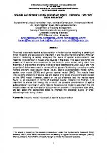
(a) (Reproduced from [10]) Worldwide climatic impacts of warm El Nino events during the northern hemisphere winter
(b) Angle of Time Series in Two Cones
Fig. 1. El Nino Effects and Cones
The climate of the Earth’s land surface is strongly influenced by the behavior of the oceans. Simultaneous variations in climate and related processes over widely separated points on the Earth are called teleconnections. For example, every three to seven years, an El Nino event [1], i.e., the anomalous warming of the eastern tropical region of the Pacific Ocean, may last for months, having significant economic and atmospheric consequences worldwide. El Nino has been linked to climate phenomena such as droughts in Australia and heavy rainfall along the eastern coast of South America, as shown in Figure 1 (a). D indicates drought, R indicates unusually high rainfall (not necessarily unusually intense rainfall) and W indicates abnormally warm periods. To investigate such landsea teleconnections, time series correlation analysis across the land and ocean is often used to reveal the relationship of measurements of observations. For example, the identification of teleconnections between Minneapolis and the eastern tropical region of the Pacific Ocean would help Earth scientists to better understand and predict the influence of El Nino in Minneapolis. In our example, the query time series is the monthly NPP data in Minneapolis from 1982 to 1993, denoted as Tq . The minimal correlation threshold is denoted as θ. This is a correlation-based similarity range query to retrieve all highly correlated SST time series in the eastern tropical region of the Pacific Ocean with the NPP time series in Minneapolis. We carry out the range query to retrieve all time series which correlate with Tq over θ in the spatial time series data S, which contain all the SST time series data in the eastern tropical region of the Pacific Ocean from 1982 to 1993. The table design of S could be represented as shown in Table 1. This query is represented using SQL as follows: select SST from S where correlation(SST,Tq ) ≥ θ
S: SST of the Eastern Pacific Ocean N: NPP of Minnesota Longitude Latitude SST (82-93) Longitude Latitude NPP (82-93) Table 1. Tables Schema for Table S and Table N
Another interesting example query is to retrieve all the highly correlated SST time series in the eastern tropical region of the Pacific with the time series of NPP in all of Minnesota. This query is a correlation-based similarity join between the NPP of Minnesota land grids and the SST in the eastern tropical region of the Pacific. The table design of Minnesota NPP time series data from 1982 to 1993, N , is shown in Table 1. The query is represented using SQL as follows: select NPP, SST from N, S where correlation(NPP,SST) ≥ θ Due to large amount of data available, the performance of naive nested loop algorithms is not sufficient to satisfy the increasing demands to efficiently process correlation-based similarity queries in large spatial time series datasets. We propose algorithms that use spatial autocorrelation-based search trees to facilitate the correlation-based similarity query processing in spatial time series data. Scope and Outline In this paper we choose a simple quad-tree like structure as the search tree due to its simplicity. R-tree, k-d tree, z-ordering tree and their variations [16, 19, 18] could be other possible candidates of the search tree. However, the comparison of these spatial data structures is beyond the scope of this paper. We focus on the strategies for correlation-based similarity queries in spatial time series data, and the computation saving methods we examine involve reduction of the time series pairs to be tested. Query processing using other similarity measures and computation saving methods based on non-spatial properties ( e.g. time series power spectrum [2, 6, 9]) are beyond the scope of the paper and will be addressed in future work. The rest of the paper is organized as follows. In Section 2, the basic concepts and lemmas related to the cone definition and boundaries are provided. Section 3 describes the formation of the spatial autocorrelation-based search tree and the correlation-based similarity range query and join strategies using the proposed spatial autocorrelation-based search tree. The cost models are discussed in Section 4. Section 5 presents the experimental design and results. We summarize our work and discuss future directions in Section 6.
2
Basic Concepts
Let x = hx1 , x2 , . . . , xm i and y = hy1 , y2 , . . . , ym i be two time series of length m. The correlation coefficient [5] of the two time series is defined as: corr(x, y) =
1 m−1
Pm
Pm
yi −y xi −x i=1 ( σx )· ( σy )
i=1 yi , m
σy =
q Pm
= x b· yb, where x =
2 i=1 (yi −x) , m−1
xbi =
Pm i=1
m
xi −x √ 1 , m−1 σx
xi
, σx =
ybi =
q Pm
2 i=1 (xi −x)
m−1
, y =
yi −y √ 1 , x b = hb x1 , x b2 , m−1 σy of the xbi 2 is equal to 1:
.P .. ,x bm i, and yb = hb y1 , yb2 , . . . , ybm i. Because the sum Pm m 2 1 √ r P xi −x x b = ( )2 = 1, x b is located in a multi-dimensional i=1 i i=1 m 2 m−1 (x −x) i=1 i m−1
unit sphere. Similarly, yb is also located in a multi-dimensional unit sphere. Based on the definition of corr(x, y), we have corr(x, y) = x b· yb = cos(∠(b x, yb)). The correlation of two time series is directly related to the angle between the two time series in the multi-dimensional unit sphere. Finding pairs of time series with an absolute value of correlation above the user given minimal correlation threshold θ is equivalent to finding pairs of time series x b and yb on the unit multi-dimensional sphere with an angle in the range of [0, θa ] or [180◦ − θa , 180◦ ] [23]. A cone is a set of time series in a multi-dimensional unit sphere and is characterized by two parameters, the center and the span of the cone. The center of the cone is the mean of all the time series in the cone. The span τ of the cone is the maximal angle between any time series in the cone and the cone center. The largest angle(∠P1 OQ1 ) between two cones C1 and C2 is denoted as γmax and the smallest angle (∠P2 OQ2 ) is denoted as γmin , as illustrated in Figure 1 (b). We have proved that if γmax and γmin are in specific ranges, the absolute value of the correlation of any pair of time series from the two cones are all above θ (or below θ) [23]. Thus all pairs of time series between the two cones satisfy (or dissatisfy) the minimal correlation threshold. To be more specific, if we let C1 and C2 be two cones from the multi-dimensional unit sphere structure and let x b and yb be any two time series from the two cones respectively, we have the following properties(please refer to [23] for proof details): 1. If 0 ≤ γmax ≤ θa , then 0 ≤ ∠(b x, yb) ≤ θa . 2. If 180◦ − θa ≤ γmin ≤ 180◦ , then 180◦ − θa ≤ ∠(b x, yb) ≤ 180◦ . ◦ ◦ 3. If θa ≤ γmin ≤ 180 and γmin ≤ γmax ≤ 180 − θa , then θa ≤ ∠(b x, yb) ≤ 180◦ − θa If either of the first two conditions is satisfied, {C1 , C2 } is called an All-True cone pair (All-True lemma). If the third condition is satisfied, {C1 , C2 } is called an All-False cone pair (All-False lemma).
3
Strategies for Correlation-Based Similarity Queries
In this section, we describe the formation of a spatial autocorrelation-based search tree and strategies for processing correlation-based similarity range queries and joins using the proposed search tree. 3.1
Spatial Autocorrelation-Based Search Tree Formation
We explore spatial autocorrelation, i.e., the influence of neighboring regions on each other, to form a search tree. Search tree structures have been widely used
in traditional DBMS (e.g. B-tree and B+ tree) and spatial DBMS (quad-tree, R-tree, R+ -tree, R*-tree, and R-link tree [16, 19] ). To fully exploit the spatial autocorrelation property, there are three major criteria for choosing a tree on the spatial time series datasets. First, a spatial tree structure is preferred to incorporate the spatial component of the datasets. Second, during the tree formation the time series calculations such as mean and span should be minimized while still need to maintain a high correlation (high clustering) among time series within a tree node. Third, threaded leaves where leaves are linked are preferred to support sequential scan of files which are useful for high selectivity ratio correlation queries. Other desired properties include depth balances of a tree and incremental updates when the time series component changes. Algorithm 1 Spatial Similarity Search Tree Formation Input: 1) S = {s1 , s2 , . . . , sn } : n spatial referenced time series where each instance references a spatial framework SF ; 2) a maximum threshold of cone angle τmax Output: Similarity Search Tree with Threaded Leaves Method: divide SF into a collection of disjoint cells C /* each cell is mapped to a cone. */ index = 1; while (index < C.size) C(index).cener = Calculate Center(C, index); /* cone center is the average time series within the cone. */ C(index).angle = Calculate Span(C, index); /* cone span is the max angle between any time series and the cone center within the cone. */ if ( C(index).angle > τmax ) split cell C(index) into four quarters C11 , C12 ,C13 ,C14 ; insert four quarters into C at position index + 1; set C11 , C12 ,C13 ,C14 as C(index)’s children; else index ++ ; insert C(index) at the end of the threaded leaf list; return C;
We choose a simple quad tree with threaded leaves which satisfies the three criteria. Other tree structures are also possible and will be explored in future work. As shown in Algorithm 1, the space is first divided into a collection of disjoint cells with a coarse starting resolution. Each cell represents a cone in the multi-dimensional unit sphere representation and includes multiple time series . Then the center and span are calculated to characterize each cone. When the cone span exceeds the maximal span threshold, this cone is split into four quarters. Each quarter is checked and split recursively until the cone span is less than the maximal span.
The maximal span threshold can be estimated by using an algebraic formula analyzed as follows. Given a minimal correlation threshold θ (0 < θ < 1), γmax = δ + τ1 + τ2 and γmin = δ − τ1 − τ2 , where δ is the angle between the centers of two cones, and the τ1 and τ2 are the spans of the two cones respectively. For simplicity, suppose τ1 ' τ2 = τ . We have the following two properties (Please refer to [23] for proof details): 1. Given a minimal correlation threshold θ, if a pair of cones both with span τ . is an All-True cone pair, then τ < arccos(θ) 2 2. Given a minimal correlation threshold θ, if a pair of cones both with span τ ◦ arccos(θ) is an All-False cone pair, then τ < 180 . 4 − 2 We use the above two properties to develop a heuristic to bound the maximal span of a cone. The maximal span of a cone is set to be the minimal of the arccos(θ) 2 ◦ arccos(θ) and 180 − . 4 2 The starting resolution can be investigated by using a spatial correlogram [7]. A spatial correlogram plots the average correlation of pairs of spatial time series with the same spatial distance against the spatial distances of those pairs. We choose the starting resolution size whose average correlation is close to the ◦ arccos(θ) correlation which corresponds to min( arccos(θ) , 180 ). 2 4 − 2 (a)
(b)
(c)
Land Cell
(d)
Ocean Cells O1
L2
L1
O2
L2
0
0 O
O11
1
1 O2
L
2
2
3 L3
O
3 0
1
2
3
L4
L1
L2
L3
L
(a)(c) Direction Vectors Attached to Spatial Frameworks (Dotted Rectangles Represent Four Quarters after Splitting)
L4
O3
0
1
2
3
O4
O1
O2
O3
O4
O
(b)(d) Selective Cones in Unit Circle and Spatial Autocorrelation-based Search Trees for L and O (Dim = 2, Multi-dimensional Sphere Reduces to Circle
Fig. 2. An Illustrative Example for Spatial Autocorrelation-Based Search Tree Formation
Example 1 (Spatial Autocorrelation-Based Search Tree Formation). Figure 2 illustrates the spatial autocorrelation-based search tree formation for two datasets, namely land and ocean. Each land/ocean framework consists of 16 locations on the starting resolution. The time series of length m in a location s is denoted as F (s) = F1 (s), F2 (s), . . . , Fi (s), . . . Fm (s). Figure 2 only depicts a time series for m = 2. Each arrow in a location s of ocean or land represents the vector < F1 (s), F2 (s) > normalized to the two dimensional unit sphere. Since the dimension of the time series is two, the multi-dimensional unit sphere reduces to a unit circle, as shown in Figure 2 (b) and (d).
Both land and ocean cells are further split into four quarters respectively due to the spatial heterogeneity in the cell. The land is partitioned to L1 − L4 and the ocean is partitioned to O1 − O4 , as shown in Figure 2 (a) and (c). Each quarter represents a cone in the multi-dimensional unit sphere. For example, the patch L2 in Figure 2 (a) matches L2 in the circle in Figure 2 (b). All leaves are threaded, assuming that L1 to L4 and O1 to O4 are all leaves. 3.2
Strategies for Similarity Range Queries and Similarity Joins
The first step is to pre-process the raw data to the multi-dimensional unit sphere representation. The second step, formation of spatial autocorrelationbased search trees involves grouping similar time series into hierarchical cones using the one described in Algorithm 1. The query processing functions called may be related to similarity range query or similarity join, depending on the query types. Algorithm 2 Correlation-Based Similarity Query Algorithm Input: 1) S 1 = {s11 , s12 , . . . , s1n1 }: n1 spatial referenced time series where each instance references a spatial framework SF1 ; 2) S 2 = {s21 , s22 , . . . , s2n2 }: n2 spatial referenced time series where each instance references a spatial framework SF2 ; 3) a user defined correlation threshold θ; 4) query time series denote Tq ; 1 5) a maximum threshold of cone angle τmax 2 6) a maximum threshold of cone angle τmax Output: pairs of time series each from S 1 and S 2 or Tq and S 2 with correlations above θ; Method: Pre-processing(S 1 ); Pre-processing(S 2 ); (1) 1 T1 = Spatial Similarity Search Tree Formation(S 1 , τmax ); (2) 2 T2 = Spatial Similarity Search Tree Formation(S 2 , τmax ); (3) if range query (4) /* assume to find highly correlated time series with Tq in S 2 .*/ (5) Similarity Range Query(T2 ,Tq , θ); (6) else if similarity join (7) Similarity Join(T1 ,T2 ,θ); (8)
Strategies for Range Queries Given a query time series Tq , we want to search all highly correlated time series from the spatial time series dataset S 2 with Tq . In general, strategies to process range queries include scan-based approaches and search tree-based approaches [8]. The scan-based approaches probe each individual nodes one by one. The search tree-based approach starts from the root of the tree and branches to a node’s children only when certain conditions
are satisfied, e.g., the minimal bounding box of the child contains the querying element. Algorithm 3 Similarity Range Query Input: 1) T : a spatial autocorrelation-based search tree with threaded leaves; 2) Tq : the query time series denote; 3) a user defined correlation threshold θ; Output: all time series each from S whose correlations with Tq are above θ; Method: traverse T ; for each cone c on the route do (1) F ilter F lag = Cone-level Join(Tq , c, θ); (2) if (F ilter F lag == ALL TRUE) (3) output all time series in the cone c (4) else if (F ilter F lag != ALL FALSE) (5) if c is a leaf node (6) for all pair Tq and s from c do (7) High Corr F lag = Instance-level Join(Tq ,s, θ); (8) if (High Corr F lag) output s; (9) else for each c0 of c’s children do (10) Similarity Range Query(c0 , Tq , θ) (11)
We adopt two common strategies to traverse the spatial autocorrelationbased search tree (step 1), namely threaded-leaves-only strategy and tree-based strategy. Note that the query time series Tq can be treated as a cone with a cone span 0. The threaded-leaves-only traversal only visits all the leaf nodes of the tree. The pairs of time series formed by T1 and each time series in a leaf node which satisfies the All-True lemma will be output. The pairs of time series formed by T1 and each time series in a leaf node which satisfies the All-False lemma will be ignored. An individual time series in a leave node which fails both All-True and All-False lemmas will be visited. The tree-based traversal starts from the root and checks the All-True and All-False lemmas. The children of non-leaf nodes which fail both All-True and All-False lemmas will be visited until a leaf node is reached. For leaf nodes, the process is the same as that in the threaded-leaves-only traversal. Example 2 (A Similarity Range Query). The range query with respect to O11 and L in Figure 2 (a) and (c) is applied as shown in Table 2. For the threadedleaves-only traversal, all leaf cones are checked against O11 for correlation. The total cost is the sum of 4, which is the filtering cost, and 4, which is the refinement cost. For the tree-based traversal, O11 is first checked with L against the AllTrue and All-False lemmas. If both of them fail, all of L’s four children, which are all leaf nodes, are checked. Three of them satisfy the All-False Lemmas and one needs refinement where individual time series are checked against O11 for
correlation. The total correlation computation is the sum of 5 and 4, which is the refinement cost. For this particular example, the tree-based traversal is more expensive than the threaded-leaves-only traversal.
Tree-Based Traversal Threaded-leaves-only Traversal Ocean-Land Filtering Refinement Ocean-Land Filtering Refinement O11 − L No No O11 − L1 No 4 O11 − L1 No 4 O11 − L2 All-False O11 − L2 All-False O11 − L3 All-False O11 − L2 All-False O11 − L4 All-False O11 − L2 All-False Table 2. The Range Query with Respect to O11 in Example Data
Strategies for Similarity Joins Spatial join operations are usually divided into a filter step and a refinement step [19] to efficiently process complex spatial data types such as point collections. In the filter step, the spatial objects are represented by simpler approximations such as the MBR (Minimum Bounding Rectangle). There are several well-known algorithms, such as plane sweep [3], space partition [13] and tree matching [14], which can then be used for computing the spatial join of MBRs using the overlap relationship; the answers from this test form the candidate solution set. In the refinement step, the exact geometry of each element from the candidate set and the exact spatial predicates are examined along with the combinatorial predicate to obtain the final result. For a join between two spatial autocorrelation-based search trees, we traverse one tree in a threaded-leaves-only manner and traverse the other tree in either a threaded-leaves-only manner (single loop join) or a tree-based manner(nested loop join). Other traversal combinations such as tree matching are also possible but are beyond the scope of this paper; they will be addressed in future work. For each leaf c1 in the first search tree, a process similar to the range query with respect to c1 is carried out. Example 3 (A Similarity Join). The join operation between the cones in Figure 2 (a) and (c) is applied as shown in Table 3. For the nested loop join, each leaf ocean cone is checked with the land cones. The cost of the threaded-leaves-only traversal is the sum of 16, which is the filtering cost, and 2 × 16, which is the refinement cost. For the single loop join, each ocean cone is checked with the land cones starting with the root L. Its children will be visited only if neither the All-True or All-False lemmas turns out to be true. As can be seen, some All-False cone pairs and All-True cone pairs are detected in the non-leaf nodes and their descendents are not visited at all. The cost of the tree-based traversal is the sum of 12, which is the filtering cost, and 2 × 16, which is the refinement cost.
Algorithm 4 Similarity Join Input: 1) T 1 : a spatial autocorrelation-based search tree with threaded leaves ; 2) T 2 : a spatial autocorrelation-based search tree with threaded leaves; 3) a user defined correlation threshold θ; Output: all pairs of time series each from leaves of C 1 and C 2 with correlations above θ; Method: traverse T1 via threaded leaves; for each c1 from T1 do (1) traverse T2 ; for each c2 T2 do (2) (3) F ilter F lag = Cone-level Join(c1 , c2 , θ); if (F ilter F lag == ALL TRUE) (4) output all pairs in the two cones (5) else if (F ilter F lag != ALL FALSE) (6) if c2 is a leaf node (7) for all pair s1 from c1 and s from c do (8) High Corr F lag = Instance-level Join(s1 ,s2 , θ); (9) if (High Corr F lag) output s1 and s2 ; (10) else for each c0 of c’s children do (11) Similarity Join(c1 , c0 , θ) (12)
Tree-Based Traversal Threaded-leaves-only Traversal Ocean-Land Filtering Refinement Ocean-Land Filtering Refinement O1 − L No O1 − L 1 No 16 O1 − L 1 No 16 O1 − L2 All-False O1 − L2 All-False O1 − L3 All-False O1 − L3 All-False O1 − L4 All-False O1 − L4 All-False O2 − L All-False O2 − L1 All-True O2 − L2 All-True O2 − L3 All-True O2 − L4 All-True O3 − L No O3 − L1 All-True O3 − L1 All-True O3 − L2 All-True O3 − L2 All-True O3 − L3 All-True O3 − L3 All-True O3 − L 4 No 16 O3 − L 4 No 16 O4 − L4 All-True O4 − L1 All-True O4 − L2 All-True O4 − L3 All-True O4 − L4 All-True Table 3. Join in Example Data
Lemma 1 (Completeness and Correctness of the Range Query Algorithm). The Similarity Range Query algorithm is complete and correct. Proof Sketch: Given a query time series Tq , for the threaded-leaves-only traversal, a pair of time series Tq and T 0 having a correlation value greater than the user given threshold can only be dismissed when it is in a pair of cones satisfying the AllFalse lemma or in Instance-level Join (step 8 in Algorithm 3). The All-False lemma ensures no false-dismissal in the first case and the instance level pairwise checking will not false dismiss either. Any pair of time series found having a correlation value greater than the user given threshold either comes from an AllTrue cone pair (step 4 in Algorithm 3) or from individual correlation checking (step 9 in Algorithm 3). The All-True lemma ensures no false-admission in the first case and the individual checking will not false admit any pair either. Given a query time series Tq , for the tree-based traversal, pairs formed by Tq and individual time series in a non-leaf node will be output if they satisfy the All-True lemma; pairs formed by Tq and individual time series in a non-leaf node will be dismissed if they satisfied the All-False lemma. The children will not be visited in both of these cases. This will not result in a false dismissal or false admission for any pair because of the All-True, All-False lemmas and the fact that the union of the time series sets of a non-leaf node’s children is the same as the time series set of their parent. The children of a non-leaf node which does not satisfy the two lemma will be visited recursively. As in the threaded-leaves-only traversal, the leaf node will also be checked against the All-True and All-False lemmas. The completeness and correctness can be argued similarly. Lemma 2 (Completeness and Correctness of the Join Algorithm). The Similarity Join algorithm is complete and correct. Proof Sketch: The Similarity Join algorithm is similar to the Similarity Range Query algorithm with a set of query time series organized as threaded leaves. The completeness and correctness proofs are similar to those in Lemma 1.
4
Cost Models
In this section, we provide simple algebraic cost models for correlation-based similarity range queries and joins(all-pair queries) in spatial time series datasets. The correlation analysis of spatial time series is a CPU intensive task, and the CPU cost is at least as important as the I/O cost for datasets with a long sequence of time series. Furthermore, the number of correlation computations could also be used to measure the computational cost of correlation analyses in different system configurations. Therefore, the number of correlation computations is used as the unit of cost in the cost models. We will investigate a cost model that includes the I/O cost of query processing in spatial time series data in future work.
As we discussed in Section 3, the proposed algorithms for correlation-based similarity queries include the construction of a similarity search tree and query processing using the spatial autocorrelation based search tree. Therefore the cost model of a correlation based similarity query, Cost, consists of Costconstruct tree , the cost of the formation of the similarity search tree for data, and Costquery , the cost of query processing. We denote the fraction of leaf cones satisfying the All-True or All-False lemmas as F AR (the filter ability ratio). The cost models for similarity range queries and similarity joins are introduced respectively in the following subsections. 4.1
Cost Models for Correlation-based Similarity Range Queries
Let Tq be the query time series and the objective of the correlation-based similarity range queries be to retrieve all highly correlated time series with Tq from a spatial time series data S. As discussed in Section 3, there are two query strategies for similarity range queries: matching using a threaded-leaves-only traversal and matching using a tree-based traversal. The costs of the formation of the search tree are the same for the two range query strategies, denoted as Costconstruct tree . Let T denote the search tree for the dataset S and |T | denote the number of nodes in T . Assume the average number of the time series in a leaf cone is nl . We discuss the cost of query processing for the similarity range queries using the two strategies as follows. The threaded-leaf-only strategy scans all leaf cones linearly, and prunes all All-True and All-False cones. Let F ARthreaded leaf , which denotes the filtering ability ratio for this strategy, represent the percentage of All-True and All-False cones in all leaf cones. Let L denote the threaded leaf cone set in the search tree and |L| denote the number of leaf cones in L. This strategy scans each leaf cone once, and the refinements occur for the cones which cannot be filtered. The cost of the refinement step is |L| × (1 − F ARthreaded leaf ) × nl . Therefore the cost of query processing for this strategy is: leaf Costthreaded range query = |L| + |L| × (1 − F ARthreaded leaf ) × nl
The tree-based strategy traverses all branches in the search tree. It stops traversing when the root cone of this subtree is an All-True or All-False or leaf cone. Let Nt denote all the nodes(cones) visited in the tree-based traversal and |Nt | denote the number of nodes in Nt . Let F ARtree based , which denotes the leave node filtering ability ratio for this strategy, represent the percentage of All-True and All-False cones in all visited leaf nodes. The cost of the refinement step is |L| × (1 − F ARtree based ) × nl . Therefore the cost of query processing for this strategy is: based Costtree range query = |Nt | + |L| × (1 − F ARtree based ) × nl
Since both strategies construct the same search trees, the filtering ability ratios are the same for the range query processing using the two strategies, i.e., F ARthreaded leaf = F ARtree based . Hence the costs of the refinement step for
the two strategies are the same. When the filtering ability ratio of a range query increases, the number of nodes visited using the tree-based strategy, |Nt | often tends to decrease. 4.2
Cost Models for Correlation-based Similarity Joins
Let S1 and S2 be two spatial time series datasets. The objective of the correlation based similarity join is to retrieve all highly correlated time series pairs between the two datasets. As discussed in Section 3, there are two query strategies for a similarity join: the nested loop approach, which iterates the threaded leaves of both search trees, and the single loop approach, which iterates the threaded leaves of one search tree and traverses the other search tree in a checking and branching manner. The costs of the formation of search trees denoted as Costconstruct tree are the same for the two join strategies. Let T1 and T2 denote the search trees for the dataset S1 and S2 respectively. Let |T1 | and |T2 | denote the number of nodes in T1 and T2 respectively. Let L1 and L2 be the leaf cone sets for T1 and T2 respectively, and |L1 | and |L2 | be the number of leaf cones in L1 and L2 respectively. Assume the average numbers of the time series in leaf cones are nl1 and nl2 for L1 and L2 respectively. We will discuss the cost of the query processing for the join processing using the two strategies as follows. The strategy using a nested loop of the threaded leaf cones is a cone-level join between two leaf cone sets of the two search trees. Let F ARnested loop , which denotes the filtering ability ratio for this strategy, represent the percentage of All-True and All-False cones in the nested loop join. The cost of the nested loop join is |L1 | × |L2 |, and the cost of refinement is |L1 | × |L2 | × (1 − F ARnested loop ). The total cost of join processing using the nested loop of leaf cones is: loop Costnested = |L1 | × |L2 | + |L1 | × |L2 | × (1 − F ARnested loop ) × nl1 × nl2 join
The strategy using a single loop of tree-based traversal chooses the search tree with the smaller number of leaf cones as the outer loop, and choose the other as the search tree in the inner loop. Without losing the generality, we assume that the leaf cone set of T1 is chosen as the outer loop and T2 is chosen as the search tree in the inner loop. Let Nt2 denote all the visited nodes in the search tree T2 and |Nt2 | denote the number of nodes in Nt2 . Let F ARtree based , which denotes the leaf node filtering ability ratio for this strategy, represent the percentage of All-True and All-False cones of the leaf nodes in the nested loop join. We match each leaf cone center in the outer loop with the inner search tree T2 . Therefore each matching is a special range query for each leaf cone with multiple time series inside, and the cost is |Nt2 |+|L2 |×F ARsingle loop ×nl1 ×nl2 The total cost of the joins using the single loop is: single loop Costjoin = |L1 | × (|Nt2 | + |L2 | × (1 − F ARsingle loop ) × nl1 × nl2 )
5
Performance Evaluation
We wanted to answer two questions: (1) How do the two query strategies improve the performance of correlation-based similarity range query processing?
Pre-Processing
Spatial Autocorrelation-based Search Tree Construction
(2) How do the two query strategies improve the performance of correlation based similarity join processing?
spatial time series 1
initial cone size 1 Threaded Leaves only Traversal join
+ Pre-Processing
Filtering
+
Refinement
Threaded Leaves only Traversal Search Tree Construction
Spatial Autocorrelation-based
Pre-Processing
range query time series spatial time series 2
minimal correlation threshold
range query
+
+ initial cone size 2
All-True
All-False
Answers
Tree-based Traversal
Note:
+
represents the multiple choices
Fig. 3. Experimental Design
We evaluated the performance of the proposed query processing strategies with a dataset from NASA Earth science data [15]. In this experiment, correlationbased similarity queries were carried out between the Sea Surface Temperature (SST) in the eastern tropical region of the Pacific Ocean(80W - 180W, 15N 15S) and Net Primary Production (NPP) in the United States. The NPP time series from 2901 land cells of the United States and the SST time series from 11556 ocean cells of the eastern tropical region of the Pacific Ocean were obtained under a 0.5 degree by 0.5 degree resolution. The records of NPP and SST were monthly data from 1982 to 1993. Figure 3 describes the experimental setup to evaluate the different strategies for similarity range query and join processing. As we noted in Section 3, there are two proposed strategies for the query processing: threaded-leaves-only traversal and tree-based traversal. We investigated the two strategies for range similarity queries. For the similarity joins, we chose the threaded-leaves-only traversal for the outer loop, and we evaluated the two query strategies in the search tree of the inner loop. Here we briefly discuss the selection of parameters for the experiments. As we stated in Section 3, the range of the maximum threshold of cone angles, τmax , is related to the minimal correlation thresholds θ and it is bounded by the minimal ◦ arccos(θ) of the arccos(θ) and 180 . In our application domain, one of constrains 2 4 − 2 is the need for fast search tree construction. We begin with the construction of a search tree using a starting cone size. The starting cone sizes depend on the nature of the data and can be roughly estimated using correlograms. The spatial correlogram plots the average correlation of pairs of spatial time series
1
1 0.99 0.98 0.97 0.96 0.95
0.95
0.9 0.9
Correlation
Correlation
0.85
0.8
0.85
0.75 0.8 0.7 0.75 0.65
0.6
1 2 3 4 5 6 7 8 9 10 11 12 13 14 15
20
25
30
Distance
(a) Correlogram for Land
35
1 2 3 4 5 6 7 8 9 10 11 12 13 14 15
20
25
30
35
Distance
(b) Correlogram for Ocean
Fig. 4. Empirical Correlograms for Land and Ocean Samples
with same spatial distance against the spatial distances of those pairs. A coarse starting cone size is enough to construct the spatial autocorrelation-based search tree. Figure 4 represents the correlograms of samples from the eastern tropical region of the Pacific Ocean and the United States and illustrates the relationships between the pairwise distances and correlations among the samples. The x-axis represents the distances of the ocean-ocean/land-land pairs in the unit of degree, and the y-axis represents the correlations of the time series of the ocean-ocean/land-land pairs. According to this figure, the ocean demonstrates higher spatial autocorrelation than the land. The land does not show as strong spatial autocorrelation as the ocean, and we will vary the starting cone size only for the eastern tropical Pacific Ocean in the experiment for simplicity. The land cone size was fixed at 1 × 1. 5.1
Correlation-based Similarity Range Query Processing
This section describes a group of queries carried out to show the savings of the two strategies for a correlation-based range similarity queries. The SST data for the eastern tropical region of the Pacific ocean was chosen as the inner loop to construct a spatial autocorrelation-based search tree. The query time series were from the NPP data in the United States. We carried out the range queries in the spatial autocorrelation-based search tree for SST. All time series in SST, which correlates with the query NPP time series over the given minimal correlation threshold θ, are retrieved. We chose the starting cone size for the eastern tropical region of the Pacific Ocean to be 8 × 8. (Assume that we have built the spatial autocorrelation-based search tree for the SST time series in the inner loop before we carried out the queries.) The brute force strategy scans all the time series in SST linearly. The cost of the brute force range queries is equal to |SST |, where |SST | denotes the number of time series in the SST data. Here we define the saving ratio as the
Title: Average Saving Ratios of 10 Range Queries Average Saving Ratios
0.9 0.8 0.7 0.6 0.5 0.4 0.3
Leaf Only Traversal Tree−based Traversal 0.4
0.5
0.6
0.7
0.8
0.9
0.8
0.9
Average Selectivity Ratios
Minimial Correlation Thresholds of Range Query Title: Average Selectivity Ratios of 10 Range Queries 0.4
0.3
0.2
0.1
0 0.3
0.4
0.5
0.6
0.7
Minimial Correlation Thresholds of Range Query
Fig. 5. Savings and Selectivity Ratios for Range Query Processing
percentage of cost savings of a range query processing compared to the cost of a range query using the brute force strategy measured in the unit of number of correlation computations. And we define the average saving ratio for multiple range queries as the mean saving ratio for these range queries. We define the selectivity ratio for a range query as the fraction of query results of time series among all the time series in the dataset. And we define the average selectivity ratio for multiple range queries as the mean selectivity ratio for these range queries. We randomly chose 10 NPP time series from the United States and carried out the correlation-based similarity range queries using the two different strategies respectively with the SST data from the eastern tropical region of the Pacific Ocean. The geographical locations of the 10 query time series were widely spread in the United States. The average selectivity ratios for the 10 queries at the different minimal correlation thresholds are illustrated in the lower plot of Figure 5. As the minimal correlation threshold increased from 0.3 to 0.9, the average selectivity ratio decreased from 0.4 to 0. The average saving ratios using the two query strategies for the 10 queries at the different minimal correlation thresholds (0.3-0.9) are presented in the upper plot of Figure 5. The solid line represents the average saving ratios for the threaded-leaves-only traversal strategy, which range from 0.46 to 0.80. The dash-dot line represents the average saving ratios for the tree-based traversal strategy, and the saving ratios range from 0.48 to 0.89. As the selectivity ratio decreases, more and more non-leaf nodes(cones) in the search tree are identified as All-True or All-False cones in the query processing using the tree-based strategy. Thus the tree-based strategy often outperformed the threaded-leaves-only strategy as the selectivity ratio decreased.
5.2
Correlation-based Similarity Join Processing
This section describes a group of experiments carried out to show the net savings of the two strategies for the correlation-based similarity joins. The NPP time series dataset for the United State was chosen as the outer loop. As we discussed in the selection of parameter, the cone size for the NPP data was fixed at 1 × 1. The SST time series data for the eastern tropical region of the Pacific Ocean was chosen as the inner loop. A spatial autocorrelation-based search tree was constructed for the SST data. (Assume that we have built the spatial autocorrelation-based search trees before we carried out the similarity join operations.)
1
1
0.8
0.8
Saving Ratios
Saving Ratios
Savings Ratios of Join Processing at Different Minimal Correlation Thresholds θ = 0.5 θ = 0.3
0.6 0.4 0.2 0
3
4
5
6
0.4 0.2
Leaf Only Traversal Tree−based Traversal 2
0.6
7
0
8
Leaf Only Traversal Tree−based Traversal 2
1
1
0.8
0.8
0.6 0.4 0.2 0
Leaf Only Traversal Tree−based Traversal 2
3
4
5
6
7
Starting Ocean Cone Sizes
4
5
6
7
8
Starting Ocean Cone Sizes θ = 0.9
Saving Ratios
Saving Ratios
Starting Ocean Cone Sizes θ = 0.7
3
8
0.6 0.4 0.2 0
Leaf Only Traversal Tree−based Traversal 2
3
4
5
6
7
8
Starting Ocean Cone Sizes
Fig. 6. Savings for Join Processing
The cost of a brute force strategy is |N P P |×|SST |, where |N P P | and |SST | are the number of the time series in NPP and SST respectively. Here we define the saving ratio as the percentage of cost savings of a join processing compared to the cost of a join using a brute force strategy measured in the unit of number of correlation computations. We define the selectivity ratio for a join as the fraction of join results of time series among the cross product of the two spatial time series datasets. The selectivity ratios for the join processing of the NPP data and SST data are shown in Table. 4. As the minimal correlation threshold of the joins increased from 0.3 to 0.9, the selectivity ratio decreased from 0.39 to 0. The saving ratios of the join processing using the two strategies are shown in Figure 6. Each subplot represents the saving ratios of the join processing for the
two strategies using the search tree beginning with the different starting ocean cone sizes at a fixed minimal correlation threshold. The starting cone sizes for the eastern tropical region of the Pacific Ocean vary from 2 × 2 to 8 × 8. The saving ratios were presented at the different minimal correlation thresholds as shown in Figure 6. The saving ratios of the join processing using both strategies increases as the minimal correlation threshold of the joins increases. When the selectivity ratio is high, more leaf nodes(cones) are possibly traversed in the join processing using the tree-based strategy. The threaded-leaves-only strategy often tends to outperform the tree-based strategy at a high selectivity ratio. However, the tree-based strategy often outperformed the threaded-leaves-only strategy as the selectivity ratio was decreased. Minimal Correlation Thresholds 0.3 0.4 0.5 0.6 0.7 0.8 0.9 Selectivity Ratios 0.39 0.22 0.11 0.04 0.005 0.0006 0 Table 4. Selectivity Ratios for the Join between NPP data and SST data
In summary, the experimental results show that the query processing using the two query strategies saves a large fraction of the computational cost. The performance of the query processing using the two strategies is robust to the starting cone sizes, and it offers stable savings for the different starting cone sizes.
6
Conclusion and Future Work
We investigated the processing strategies for correlation-based similarity range queries and joins using a spatial autocorrelation search tree. Algebraic cost models were proposed and evaluation and experiments with Earth science data [15] show that the performance of the query and join processing strategies using the spatial autocorrelation-based search tree structure saves a large fraction of computational cost. In future work, we would like to explore other search tree candidates, such as k-d tree, R-tree, and R-link tree. We plan to incorporate I/O costs into our cost models and carry out the comparison of experimental results with the prediction of algebraic cost models. We will also carry out a comparison study between the proposed query processing strategies with other indexing techniques [2, 6, 9] in spatial time series data.
Acknowledgments We are particularly grateful to NASA Ames Research Center collaborators C. Potter and S. Klooster for their helpful comments and valuable discussions. We would also like to express our thanks to Kim Koffolt for improving the readability of this paper.
References 1. NOAA El Nino Page. http://www.elnino.noaa.gov/. 2. R. Agrawal, C. Faloutsos, and A. Swami. Efficient Similarity Search In Sequence Databases. In Proc. of the 4th Int’l Conference of Foundations of Data Organization and Algorithms, 1993. 3. L. Arge, O. Procopiuc, S. Ramaswamy, T. Suel, and J. Vitter. Scalable SweepingBased Spatial Join. In Proc. of the 24th Int’l Conf. on VLDB, 1998. 4. G. Box, G. Jenkins, and G. Reinsel. Time Series Analysis: Forecasting and Control. Prentice Hall, 1994. 5. B.W. Lindgren. Statistical Theory (Fourth Edition). Chapman-Hall, 1998. 6. K. Chan and A. W. Fu. Efficient Time Series Matching by Wavelets. In Proc. of the 15th ICDE, 1999. 7. N. Cressie. Statistics for Spatial Data. John Wiley and Sons, 1991. 8. R. Elmasri and S. Navathe. Fundamentals of Database Systems. Addison Wesley Higher Education, 2002. 9. Christos Faloutsos. Searching Multimedia Databases By Content. Kluwer Academic Publishers, 1996. 10. Food and Agriculture Organization. Farmers brace for extreme weather conditions as El Nino effect hits Latin America and Australia . http://www.fao.org/NEWS/1997/970904-e.htm. 11. R. Grossman, C. Kamath, P. Kegelmeyer, V. Kumar, and R. Namburu, editors. Data Mining for Scientific and Engineering Applications. Kluwer Academic Publishers, ISBN: 1-4020-0033-2, 2001. 12. D. Gunopulos and G. Das. Time Series Similarity Measures and Time Series Indexing. SIGMOD Record, 30(2), 2001. 13. D. J. DeWitt J. M. Patel. Partition Based Spatial-Merge Join. In Proc. of the ACM SIGMOD Conference, 1996. 14. S. T. Leutenegger and M. A. Lopez. The Effect of Buffering on the Performance of R-Trees. In Proc. of the ICDE Conf., pp 164-171, 1998. 15. C. Potter, S. Klooster, and V. Brooks. Inter-annual Variability in Terrestrial Net Primary Production: Exploration of Trends and Controls on Regional to Global Scales. Ecosystems, 2(1):36–48, 1999. 16. P. Rigaux, M. Scholl, and A. Voisard. Spatial Databases: With Application to GIS. Morgan Kaufmann Publishers, 2001. 17. J. Roddick, K. Hornsby, and M. Spiliopoulou. An Updated Bibliography of Temporal, Spatial, and Spatio-Temporal Data Mining Research. In First Int’l Workshop TSDM, 2000. 18. H. Samet. The Design and Analysis of Spatial Data Structures. Addison-Wesley Publishing Company, Inc., 1990. 19. S. Shekhar and S. Chawla. Spatial Databases: A Tour. Prentice Hall, ISBN:0130174807, 2003. 20. S. Shekhar, S. Chawla, S. Ravada, A. Fetterer, X. Liu, and C.T. Lu. Spatial Databases: Accomplishments and Research Needs. IEEE TKDE, 11(1), 1999. 21. W.R. Tobler. Cellular Geography, Philosophy in Geography. Gale and Olsson, Eds., Dordrecht, Reidel, 1979. 22. Michael F. Worboys. GIS - A Computing Perspective. Taylor and Francis, 1995. 23. Pusheng Zhang, Yan Huang, Shashi Shekhar, and Vipin Kumar. Correlation Analysis of Spatial Time Series Datasets: A Filter-and-Refine Approach. In the Proc. of the 7th Pacific-Asia Conf. on Knowledge Discovery and Data Mining, 2003.