Scale Elements in Spatial Autocorrelation Tests By Jesús Mur F. Javier Trívez
Abstract: Moran’s I is a good test for detecting relationships of cross-sectional dependency in spatial series. However, its behavior is sensitive to the scale of the process in autoregressive series. When the coefficient of variation of the process is high, the power of the test is zero in a not unimportant range of values of the coefficient of autocorrelation. In this paper we point out some solutions and discard others. Among the latter the redimensioning of the series before resolving the I test stands out. The chapter of proposals, in no case definitive, revolves around the exploitation of the heteroskedastic structure in a series with signs of spatial autocorrelation. Address: Department of Economic Analysis. University of Zaragoza Gran Vía, 2-4 Zaragoza (50005). SPAIN E-Mail:
[email protected] Phone: +34-976-761815 Fax: +34-976-761996
40TH CONGRESS OF THE EUROPEAN REGIONAL SCIENCE ASSOCIATION BARCELONA. 30 AUGUST-2 SEPTEMBER 2000
1.- Introduction
In 1950 Moran proposed one of the most popular tools in the field of spatial statistics, the I test, which addresses a basic question: is there cross-sectional dependency in the variable or model analyzed? All the available evidence points to this being the most efficient test in this field. The aim of this paper is not to question its suitability but to highlight certain weaknesses. In particular, we point out a minor question which is the dependency of the test in relation to the scale of the series. In some circumstances, the power of Moran’s I tends towards zero when the scale of the series is high. In the following section we present the basic theory related to the test, while in the third we discuss the specific problems derived from scale. In the fourth section we present some alternatives capable of lessening these difficulties, checked in the replication carried out in the fifth section. The work ends with the sixth section dedicated to the presentation of the principal conclusions reached. 2.- Basic Aspects Moran’s test, as Arbia (1989) indicates, is not a coefficient of correlation but a statistic whose objective is to measure the degree of spatial autocorrelation that exists in the spatial distribution of a variable. Its expression is well known: R
I=
R S0
∑ ( yr − y) w rs ( ys − y) r ,s
∑ (y r − y ) R
(2.1)
2
r =1
with {yr, r =1, 2, ..., R} the observations of the variable y in the R points of the space and y its corresponding sampling mean, wrs (r,s =1, 2, ..., R) the elements of the specified contiguity matrix W, with S0 = ∑ w rs . This statistic will take values in the r ,s
interval ((R/S0)mmin, (R/S0)mmax), with mmin and mmax the lowest and highest roots respectively of the matrix DWD with D=[I-(ll’/R)] where l is an (Rx1) vector of ones and I is the identity matrix (De Jong et al, 1984). If the spatial distribution of variable is random, Moran’s I will take values close to zero. Cliff and Ord (1972 and 1981) obtain the moments of the test under the null hypothesis of independence both under the normality assumption and when the distribution of the series is unknown (randomization assumption). The same authors show that, once again under the hypothesis of independence, the test tends 1
asymptotically towards the normal distribution. The conditions that guarantee this approximation are relatively weak, as can be seen in Sen (1976). Using numerical integration methods we can obtain the exact distribution function of the test (Sen, 1990, Tiefelsdorf and Boots, 1995). Furthermore, King (1981) demonstrates that the test built on Moran’s I is a Locally Best Invariant (LBI) test in the neighbourhood of the null hypothesis and, under certain conditions, a Uniformly Most Powerful Invariant (UMPI) test. Burridge (1980) obtains its formal equivalent with the Lagrange Multiplier (LM), corroborating the results put forward by Cliff and Ord (1981), while Anselin and Rey (1991) demonstrate, using Monte Carlo methods, its superiority as a test of spatial autocorrelation. All these results confer on Moran’s I test a central position in the field of spatial analysis. Nevertheless, this test presents certain limitations which it is necessary to consider. Moran’s I is insensitive to the size and the shape of the units of observation, giving rise to the problem of “topological invariance” described by Dacey (1965). This weakness is shared by practically all the spatial autocorrelation tests, with the exception of that proposed by Dacey himself. Another question is that no model is specified in the alternative hypothesis. The only clue the researcher has is that the distribution of the variable in question maintains a certain regularity in relation to the spatial structure reflected in W. Lastly, it is necessary to suppose that, under the assumption of independence, the first order moment of the variable analyzed is homogeneous in space. This is why the sampling mean is used in the definition of test in (2.1). If this assumption were unable to be maintained, the use of the normal should be rethought in favor of the focus on randomization. 3.- The Problems The principal limitation we find above is the lack of a well-defined alternative hypothesis. When the user rejects the null hypothesis of independence, it is not clear what the relevant model should be. Most applications choose an SAR structure, but there is no reason to justify this preference (why not an SMA?). This decision is generally taken with very little reasoning. An SAR process implies that the structure of dependencies in the series is of a general type, in the sense that all the regions interact with all the others without exception, however inaccessible they may be from the others. In practice this means that all the covariances should be
2
different to zero. Furthermore when an SAR process is imposed on a spatial series, we are also affirming that its expected value is not homogeneous, a characteristic that most spatial series seem to share. However, the first order moment of these processes should also respond to the spatial structure reflected in the contiguity matrix, a restriction which it does not seem very reasonable to impose in a general way. These observations have an immediate reflection in the behavior of Moran’s I. In particular, the sampling mean that intervenes in its definition will be an unbiased and consistent estimator of the expected moment when the Data Generating Process (DGP) of the series is an SMA: y = µl + (I − δW )u = µl + Bu → lim E[y] = µ E[y] = µ R →∞ l' y 2 2 y= ⇒ l ' l σ 2 W R − 2δ S0 ) → lim V[y] = 0 V[y] = (1 + δ R →∞ R R R
(3.1)
with l a vector of ones and B=I-δW. The first order moment in the SAR case is not homogeneous so the sampling mean is a statistic lacking in meaning: y = µl + δWy + u ⇒ y = B−1 (µl + u ) ⇒ E[y ] = µB−1 l
(3.2)
It is centered on the sampling mean of the expected values ( E[y] = µ(l' B−1 l) / R ), andc can be consistent in relation to this point ( lim V[y ] = σ2 (l' B−2 l) / R 2 = 0 ). R →∞
However, as an estimator of an hypothetically homogeneous factor of scale it leads to errors. In the specification of Moran’s I, the sampling mean of the series is effectively introduced to obtain both the covariance of the numerator and the variance of the denominator. The question we raise now is how Moran’s statistic responds to the scale. The comments above suggest that the inclusion of the sampling mean is justified when the DGP of the series is an SMA. If, for this type of process, we write the I statistic in matrix notation: R
I=
R S0
∑ ( yr − y) w rs ( ys − y) r ,s
∑ (y r − y ) R
2
r =1
3
=
R u ' BDWDBu S0 u ' BDBu
(3.3)
it is clear that the numerator and the denominator are quadratic forms of a vector of normal N(0,1) variates on a symmetric and singular matrix. The distribution of both quadratic forms will pertain to the chi-squared family, although they will not be independent. Using the results of Yule and Kendall (1950), we can approximate their expected value though: N E(N ) V (D) Cov ( N, D) −2 E = − 1 + + o(R ) 2 D E(D ) E(D) E( N)E(D)
(3.4)
where o(-) means “of smaller order than”. Resolving the above expression, the expected value of Moran’s I is: E[I] ≅
R trBDWDB tr (BDB)(BDB) tr (BDWDB)(BDB) − 1 + tr(BDWDB) tr(BDB) S0 trBDB ( trBDB)2
(3.5)
which can be approximated by: ∑ (1− δ λ r ) R r =1λ r E[I] ≅ 1 + R S0 ∑ (1− δ λ )2 r r =1 R
2
∑ (1− δ λ r ) ∑ λ r (1− δ λ r ) r =1 r =1 + R 2 R 2 2 R 1 − δ 1 − δ ( ) ( ) 2 ∑ ∑ λ λ λ r r r ∑ (1− δ λ r ) r =1 r =1 r =1 R
R
4
4
(3.6)
with λr the rth characteristic root of W. For positive values of the parameter δ, the expected value of I will be negative and positive for negative values of the former. The two quotients that appear in the square brackets are positive and less than one (using the Cauchy–Swartz inequality). Their contribution will become less significant as the sample size increases, so that the above expression can be reduced, for large sample sizes, to: ∑ λ r (1− δ λ r ) R
E[I] →
R
2
r =1 R
S0 ∑ (1− δ λ )2 r
(3.7)
r =1
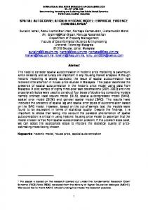
Independently of the accuracy of these approximations, the relevant aspect of all of them is that at no moment is the distribution of Moran’s I affected by the scale of the process, being efficiently neutralized by the sampling mean. The above result allows us to present graphs such as that of Figure 3.1. With the continuous line we represent the expected value of Moran’s I according to (3.7) and 4
with the dotted lines the acceptance limits of the null hypothesis of independence at a significance level of 5% (that is 1.96xDT (I), where DT(I) is the standard deviation under the null hypothesis). The reference matrix, of the order (74x74), corresponds to the NUTS II European regional system of 12 member states. The stability interval (if by such we understand that in which it is true that |δλr| 0 ⇒ l' B l > 1 ⇒ E[y] > µ R
(3.8)
In this type of process, Moran’s I can be developed as: I=
R (u + µl)' B−1 DWD B−1 (u + µl) S0 (u + µl)' B−1 D B−1 (u + µl)
(3.9)
Figure 3.1: Expected value of Moran’s I for SMA processes
Using the approximation of (3.4) again, its expected value can be expressed as: 5
E[I] ≅ −
R tr B− 2 DWD + c2 l' B−1 DWD B−1 l tr B− 2 D B− 2 D + 4 c2 l' B−1 D B− 2 D B−1 l 1 + 2 tr B2 D + c2 l' B−1 D B−1 l S0 ( tr B − 2 D + c 2 l' B −1D B −1l)
tr B−1 D B− 2 DWD B−1 + 4 c2 l' B−1 DWD B−2 D B−1 l (tr B− 2 DWD + c2 l' B−1 DWD B−1 l)(tr B− 2 D + c2 l' B−1 D B−1 l) (3.10)
with c=µ/σ2, the coefficient of variation of the process. The above result is intractable, although the probalistic limit of (3.9) can be considered as an approximation: plimI =
[
] R →∞ [ ] n1 + c2 n2 = lim [tr (B−1 D B−1) / R ]+ c2 lim [(l' B−1 D B−1 l) / R ] d1 + c2 d 2 R →∞ R →∞
lim tr(B−1 DWD B−1) / S0 + c2 lim (l' B−1 DWD B−1 l)) / S0
R →∞
(3.11)
The terms d1 and d2 are positive for any δ, while n1 and n2 will be negative for δ