1
Exploiting Task Elasticity and Price Heterogeneity for Maximizing Cloud Computing Profits Mehiar Dabbagh, Bechir Hamdaoui, Mohsen Guizani† and Ammar Rayes‡ Oregon State University, Corvallis, OR 97331, dabbaghm,
[email protected] † Qatar University,
[email protected] ‡ Cisco Systems, San Jose, CA 95134, ‡
[email protected]
I. I NTRODUCTION Maximizing profits while meeting clients’ requirements is what cloud providers aim for. Large electricity bills are being paid by cloud providers [1], merely due to a poor management of cloud resources [2–4], resulting in having servers stay unnecessarily ON for long periods while being under-utilized [5]. Therefore, to minimize the cloud’s consumed energy, one needs to reduce the number of ON servers, increase the servers utilization and reduce the duration for which servers are left ON while meeting clients’ demands. A cloud center is made up of a huge number of servers called physical machines (PMs) that are grouped into multiple management units called clusters. Cloud clients may, at any time, submit a VM request to the cloud, specifying the amount of computing resources they need to perform a certain task. Prior cloud resource management schemes focused on hanreq dling task requests of the form (wireq , treq is i ) where wi req task i’s requested amount of CPU resources and ti is the duration for which these resources are needed. Such requests are referred to by inelastic task requests as they require a fixed amount of CPU resource during their whole execution time and as increasing their allocated resources at any time would not decrease their execution times. We define the requested computing volume vireq for an inelastic task i as vireq = wireq × treq i . A cloud task request could also be elastic in that the amount of its allocated resources can be increased (or decreased) during its execution time, and doing so results in reducing (or prolonging) its execution time. An example of such tasks would be any task with thread parallelism where the number of allocated threads (CPU resources) determines how fast the task completes. An elastic task request i is defined by
PM Capacity
Index Terms—Resource allocation, VM placement, cloud computing, energy efficiency, cloud pricing.
(vireq , wimax , tmax ) where vireq is the requested computing voli ume, wimax is the maximum amount of CPU resources that can be allocated to the task, depending primarily on its maximum amount of parallelism, and tmax is a duration period by which i the task should complete. Note that the least duration needed to complete such a request is tmin = vireq /wimax , which i corresponds to allocating the maximal amount of resources wimax all the time. Thus, tmax must be strictly larger than i tmin for such a request to be feasible and elastic. i Two service models arise for handling elastic tasks: i) Best-Effort Model: clients are only interested in getting their task completed within a specified period tmax , and are charged a fixed cost based on their task’s volume. ii) Delay-Sensitive Model: not only does the task’s deadline have to be met, but also clients are willing to pay more to get their task completed earlier. 1 T1 (50%) 0.5 T2 (50%) 0 0
1
Gained Idle Time
2 3 4 Time (Hour)
5
6
(a) Allocation with minimal expenses. PM Capacity
Abstract—This paper exploits cloud task elasticity and price heterogeneity to propose an online resource management framework that maximizes cloud profits while minimizing energy expenses. This is done by reducing the duration during which servers need to be left ON and maximizing the monetary revenues when the charging cost for some of the elastic tasks depends on how fast these tasks complete, while meeting all resource requirements. Comparative studies conducted using Google data traces show the effectiveness of our proposed framework in terms of improving resource utilization, reducing energy expenses, and increasing cloud profits.
1 T1 (75%) 0.25 0
1
T2 (25%) 2 3 4 Time (Hour)
5
6
(b) Allocation with maximal revenue.
Fig. 1: Two feasible allocations for the illustrative example. The elasticity among the tasks brings further management capabilities. Exploiting these capabilities requires developing efficient scheduling techniques that decide: i) where to place the heterogeneous tasks, and ii) how much resources to allocate for each elastic task. The latter decision has a significant impact on the cloud’s monetary profits. This point can be illustrated by considering a simplified example where the cloud receives two elastic task requests, T1 and T2 , each requesting a volume of v req = 1.5, each can be allocated at most wmax = 75% of the PM’s capacity, and each must complete within tmax = 6 hours. Assume that both tasks were assigned to the same PM which has a unit capacity. There are numerous feasible ways to allocate resources for
2
T1 and T2 , and we are seeking those that maximize the cloud profits. From an expense point of view, the allocation in Fig. 1(a) meets the tasks requirements with the least cost among all possible allocations as it keeps the PM ON for the least time (3 hours only), after which the PM is turned to sleep to save energy. Of course finding the allocation with the least expenses is harder than this simplified example in real cases when many tasks (elastic and inelastic) with different computing demands are cohosted on the same PM. Things become further challenging when some of the hosted tasks are delay-sensitive as the resource allocation not only impacts the energy expenses but also determines the collected revenues. By returning to our example and considering only T1 to be a delay-sensitive task, observe that although the allocation in Fig.1(a) have lower costs than that in Fig.1(b), the latter allocation has higher revenues than the former case as T1 completes as fast as possible charging the client the highest cost. Thus the allocation in Fig.1(b) will be more profitable than that in Fig.1(a) only if the extra revenue collected for completing T1 earlier outweighs the energy cost resulting from keeping the machine on for the entire 6 hours (as opposed to 3 hours only). This makes managing cloud resources in a profitable way a challenging task. In this paper, we exploit the elasticity and the varying charging costs among the submitted tasks and propose an online resource allocation framework that aims at maximizing the cloud’s profits. To the best of our knowledge, this is the first work that exploits both of those aspects. Our main contributions are in proposing a framework that: 1) places the submitted elastic and inelastic tasks in a way that avoids turning new PMs ON while also reducing the PMs’ uptimes (i.e., the duration for which PMs need to be kept ON to serve the hosted tasks). 2) decides what amount of resources should be assigned initially to the elastic tasks while guaranteeing that their deadlines will be met. 3) tunes the amount of allocated resources for the elastic tasks over time by solving a convex optimization problem whose objective is to maximize the cloud’s profits. The remainder is organized as follows. Section II reviews prior work. Section III presents our proposed framework. Section IV proposes charging models for the elastic services. Section V describes the optimization problem solved by our framework to tune the allocations over time. Section VI evaluates our framework on real Google traces. Finally, Section VII concludes the paper and Section VIII provides directions for future work. II. R ELATED W ORK Prior resource management techniques focused on increasing the cloud profits by reducing the cloud center’s electricity bills, and can be broadly divided into two categories: A. Cluster Placement Techniques These techniques decide what cluster among the clusters that are distributed in different geographical locations should serve the submitted task requests such that the cloud center’s
energy expenses are decreased. The work in [6] exploited the temporal and spatial variations in electricity prices among the different clusters’ locations and directed the received requests to the cluster with the least power prices. The challenge here is that the electricity price exhibits significant fluctuations from a location to another over time as it is highly demand driven. Greedy heuristics [7], game-theoretical models [2], and power price estimation schemes [8] are some of the techniques that were proposed to address that challenge. The amount of generated renewable energy in each cluster’s location was also considered as a selection factor in [9] where requests were directed to the cluster with the highest reliance on green sources of energy in order to cut down both electricity costs and carbon emissions. Prediction techniques as in [10] were needed for such green selections to be effective as the amount of generated renewable energy is highly weather dependent. Quality of service requirements were also considered in [11, 12] when making cluster selections, where tasks were constrained to be placed within a certain distance from their clients in order to guarantee bounds on the client’s response time. The interested reader is referred to [13] for a complete overview on cluster selection techniques. In this paper, we consider the case where a cluster is selected to serve each submitted request using one of the previously discussed techniques [2, 6– 13]. We propose a complementary management framework for allocating task resources with the aim of reducing the cluster’s energy consumption and increasing the monetary revenues while meeting all clients computing demands. B. PM Placement Techniques These techniques aim at reducing the cluster’s energy consumption by assigning efficiently the tasks to the PMs within the cluster. The problem of finding efficient initial PM placements for the newly submitted tasks is treated as the classical online Bin Packing (BP) optimization problem [14, 15], which views the cluster’s PMs as bins with certain capacities (CPU capacities), and tasks as objects with certain sizes (CPU demands) that arrive over time, where the objective is to pack these objects in as few bins as possible. Such tight packing leads into great energy savings as it allows many redundant PMs to be switched to sleep. The online nature of the BP problem and the fact that finding the optimal solution for the offline version of that problem is NP-hard [16] encouraged using heuristics to make efficient initial PM placements. The Best Fit (BF) heuristic [17] is one of the widely used heuristics for initial PM placement in cloud centers. Enhancements over this heuristic were proposed to, for e.g., reduce communication costs [18, 19] and account for task completion times [20]. Dynamic consolidation (DC) techniques [21] improve those initial placements by using VM migration to perform periodic intra cluster VM-PM remappings, with the objective of packing the hosted VMs more tightly as some of the cluster’s PMs become highly underutilized due to the release of some of the tasks overtime. The main drawback of dynamic consolidation is that VM migration does not come for free in terms of energy consumption and performance degradation
3
Requests VM Placement
PM1
PM2
...
PMn
Resource
Resource Managmnt
...
Resource Managmnt
Managmnt
Fig. 2: Proposed Resource Allocation Framework.
[22]. To limit those negative effects of VM migration, several management schemes were proposed to decide what VMs to migrate and to which PMs in the cluster with the aim of reducing the migration energy overhead [23] or the experienced performance degradation [24]. For a complete taxonomy of prior techniques on energy efficiency in cloud centers, we refer the reader to our prior work [25]. All the techniques discussed in this category handled the case when the submitted tasks are all inelastic. To the best of our knowledge, this is the first paper that proposes a resource management framework for the case when the cluster workload is a mix of elastic and inelastic, and where the charging cost for some of the elastic tasks is dependent on how fast the tasks complete. Our proposed framework places the heterogeneous submitted tasks in a way that minimizes significantly the consumed energy with the key difference from prior placement techniques [17–19] that both the number of ON PMs and the duration for which PMs are left ON are reduced, leading to significant energy savings. Our framework then tunes the amount of allocated resources for the elastic tasks over time with the goal of increasing the profit by balancing between increasing the revenues and reducing the energy expenses while meeting all tasks demands. Unlike the dynamic consolidation techniques [21–24] which relied on VM migration to pack the workload more tightly to reduce the consumed energy, our framework exploits the elasticity among the submitted tasks and tunes the allocated resources for the hosted tasks in a way that reduces the duration for which PMs are left ON, allowing them to be turned to sleep quickly to save energy. III. T HE P ROPOSED F RAMEWORK As illustrated in Fig. 2, our proposed resource allocation framework has a two-level control structure as it is made up of a front end VM Placement module connected to all the PMs in the cloud cluster and an autonomous Resource Management module dedicated to each PM in the cluster. We explain next each one of these control modules: A. VM Placement Module Upon receiving a task request (elastic or inelastic), this module creates a VM for the submitted task and decides what PM in the cluster the created VM should be assigned to. These placement decisions are made depending on the current states of the PMs in the cluster and on two task-related quantities: the amount of CPU resources assigned initially to the created VM,
and the time after which the VM is expected to be released. In the case of an inelastic task, these two quantities are directly specified by the client to be wireq and treq respectively. On the i other hand, there is flexibility in these quantities if the task is elastic as they are only bounded above by wimax and tmax i respectively. Thus, the module needs to decide the quantity of resources that should be assigned initially to the elastic task in order to make efficient PM placement. Our module amount of resources to the elastic allocates wimin = vireq /tmax i task initially. This represents the least amount of resources needed so that the task is accomplished exactly in the client’s maximum tolerable period tmax . The intuition behind this i choice is the following. If we allocate less than wimin initially, then at some point in time we need to increase these resources so that the task terminates within tmax . However, the PM’s i capacity constraint and the constraints from the remaining hosted VMs may prevent us from doing that and thus we may risk to miss the task’s deadline. Thus at least wimin amount of resources should be allocated initially to avoid that. On the other hand, if an amount of resources larger than wimin is assigned to the VM, then there may be no ON PM with enough slack to fit that VM and we will be forced to switch a new PM from sleep to fit this VM. This switch has a high energy overhead [26, 27] and also increases the number of ON PMs which leads to high energy consumption. This costly switch will be unnecessary if an ON PM with a slack of only wimin is already available in the cluster. Thus wimin is initially allocated to the elastic task in order to guarantee meeting its deadline while also saving energy. It is worth mentioning that these are only initial assignments for the elastic tasks and will be later tuned in order to maximize the cloud profits as will be explained later. Having determined the amount of resources to be allocated initially to the submitted task’s VM and when the VM is expected to be released, we now explain the PM preference criteria that is adapted for efficient placement selection. Based on our preference criteria, the PMs in the cluster are divided into the following disjoint groups: 1) Group 1: contains all the PMs that are currently ON and that have an uptime larger than the VM’s release time. 2) Group 2: contains the remaining ON PMs (the ones with an uptime smaller than the VM’s release time). 3) Group 3: contains all the PMs in the sleep state. The module tries first to place the new task’s VM in one of the PMs of Group 1. These PMs are mostly favored as their uptime will not be increased after placing the new VM. If multiple PMs of Group 1 can fit the VM, then the one with the least CPU slack is chosen. The intuition behind this preference is to leave larger slacks on the remaining ON PMs so that VMs with larger CPU demands can be supported by these PMs in the future without needing to wake new PMs from sleep. If non of the PMs in Group 1 have enough space to fit the VM, then the PMs of Group 2 are considered. If multiple PMs from Group 2 can fit the VM, then the one whose uptime will be extended the least after placement will be chosen. This is to reduce the extra time for which the PM will be kept ON. Finally, if no fit is found in Group 2, then Group 3 is considered. Thus our preference criteria switches a new PM ON to accommodate
4
the VM only if we have no other choice. The PM in Group 3 with the largest capacity is chosen in that case so that requests with larger demands can be supported by this PM in the future. B. Resource Management Module The main role of this module is to make resource and power management decisions for the controlled PM. A PM Pj ’s module performs the following procedures: 1) Resource Allocation: A flag is dedicated to indicate whether or not the allocated resources for the tasks hosted on the controlled PM need to be retuned. This flag is set true whenever one of the following events occurs: a) a new delay-sensitive elastic task gets placed on the PM, or b) the PM’s uptime gets increased due to assigning a new best-effort elastic task, or c) one of the already hosted tasks (elastic/inelastic) gets released from the PM. The resource management module checks this flag periodically every Tp period. If the flag is true, then the amount of resources wi to be allocated to each task i hosted on Pj is tuned. This is done by solving an optimization problem whose objective is to maximize the PM’s profit, which is calculated to be the difference between the revenues collected from serving the hosted tasks and the PM’s energy expenses spent to accomplish those tasks, and where constraints are included to guarantee meeting all tasks’ requirements and deadlines. Details on the resource allocation optimization problem are provided in Section V. The flag is reset to false after updating these allocations. Ideally, to maximize the profits, new resource tuning needs to be calculated anytime a new delay-sensitive elastic task gets placed on the PM (as it might be more profitable to finish this task earlier), or any time the PM’s uptime gets extended due to assigning a new best-effort elastic task (as it might be possible to increase the allocated resources for this task so that the PM’s uptime gets decreased in order to save energy), or anytime a task gets released (as an extra free resource slack becomes available to use for the remaining hosted tasks). However, tuning the allocated resources for the hosted tasks each time one of those events occur has a high computation overhead. The flag is thus introduced for practical uses in order to limit the number of times the optimization problem is solved and the resources are retuned per PM to be once at most every Tp period. The choice of Tp is left to the cloud provider depending on how much computation overhead it can afford. The smaller the selected value for this parameter, the more responsiveness the framework becomes to tune allocations that maximize its profits, but also the higher the computation overhead. In our implementation, Tp is set to 5 minutes as evaluations revealed that high revenues and great energy savings can be achieved for such choice while keeping the calculation overhead low. 2) Remaining Time/Volume Tracking: for each elastic task i hosted on Pj , the module tracks trem , the amount of i remaining time before which the task should be accomplished. The remaining time is initially set to tmax when i
the task is first scheduled on the PM and is decremented as time goes by. For each elastic or inelastic task i hosted on Pj , the module also tracks the amount of remaining computing volume still needed to accomplish each one of these tasks. The remaining computing volume for task i, referred to by virem , is initially set to be equal to the task’s requested computing volume vireq when the task is first scheduled on Pj . Let wi be the amount of resources allocated to task i for period T , then the remaining volume will be updated after the T period is over as follows: virem ← virem − (wi × T ). 3) VM Termination: a task completes when it is allocated all of its requested computing volume. Thus the module releases the allocated resources for VM i hosted on the PM once its remaining computing volume virem reaches zero. If no other VMs are still hosted on the PM after this release, then the PM is put to sleep to save energy. IV. C HARGING M ODELS We first discuss how inelastic tasks are being charged in current cloud centers, and then propose a charging model for both the best-effort and the delay-sensitive elastic tasks. In current cloud providers (e.g. Amazon, Microsoft), the charging cost for an inelastic task i is dependent on the task’s volume vireq which captures both the amount of requested resources wireq and the duration treq for which these resources i are reserved. More specifically, letting ϕ denote the price per a unit of volume for the inelastic service, the charging cost ri for the inelastic task i can be expressed as ri = ϕ vireq
(1)
We propose a similar model for the best-effort elastic tasks with the only exception that the cloud provider charges the client’s task with a reduced price compared to the inelastic case. This is basically to provide an incentive for clients to request an inelastic service as clients in this case provide a flexibility in terms of the allocated resources and in terms of when their tasks can be accomplished. This flexibility provides further management capabilities that the cloud provider exploits to reduce its expenses and increase significantly its profits (as will be seen in Section VI), so that the reduced price for this service ends up to be a win-win situation for both the clients and the cloud provider. More specifically, the charging cost rbmin for a best-effort elastic task b with a computing volume vbreq is calculated as follows: rbmin = φ vbreq
(2)
where φ is the reduced cost per one unit of volume which is specified by the cloud provider and where φ < ϕ holds. Observe that the cost of this type of service is only dependent on the task’s volume where the cloud provider guarantees providing the requested volume to complete the task within the maximal tolerable duration tmax . It is worth mentioning b that in our model the reduced price φ was considered to be fixed for all the elastic requests. Another option could be to have a reduced price φ that is different from an elastic task to another depending on how flexible each elastic task is. The
5
Charging Cost (ri)
rmax
or a delay-sensitive elastic task. Let Bj and Dj be respectively the sets of the best-effort and the delay-sensitive elastic tasks that are hosted on Pj where Ej = Bj ∪ Dj . We explain in this section how to tune wi ∈ R++ , the amount of CPU resources to be allocated to each task i hosted on PM Pj . The allocated resources wi allows, in turn, to determine ti ∈ R++ , the time needed to accomplish the ith task. Our framework allocates resources to the tasks assigned to Pj by solving the following optimization problem.
i
rmin i
Delay−Sensitive Service Best−Effort Service min
ti
Task Duration (ti)
tmax i
Fig. 3: Proposed charging models for elastic tasks.
higher the elastic task’s flexibility, the lower the charged cost and vice versa. As for the delay-sensitive elastic tasks, the charging cost in that case is not only dependent on the task’s volume but also is affected by how fast the task completes. We propose a linear charging model for this service, where the charging cost rd of the delay-sensitive elastic task d is expressed as a function of the task’s duration td as follows: rd (td ) =
rdmin
+
δ(tmax d
− td )
(3)
Where: rdmin captures the volume cost and is calculated using equation (2), and δ is the price that the client pays for getting his task completed one unit of time earlier and is specified by the cloud provider. Recall that the duration by which the task completes td is bounded up by tmax which is the d maximal tolerable duration that is specified by the client’s request. There is also an implicit lower bound on td as the task can be allocated at most wdmax of CPU resources at any time, and thus the least duration needed to complete the task = vdreq /wdmax which corresponds to allocating the is tmin d maximal resources wdmax all the time. Observe that based on equation (3) as the task’s duration increases from tmin d , the charging cost to the maximum tolerable duration tmax d for the delay sensitive task decreases linearly from rdmax = rdmin + δ(tmax − tmin ) to rdmin . d d To further illustrate our proposed charging models, Fig. 3 plots how an elastic task i would be charged as the duration ti needed to complete the elastic task increases from tmin to i tmax for both the best-effort and the delay-sensitive services. i Observe that if task i requested a best-effort service, then its charging cost would be the same (equals to rimin ) regardless of when the task completes, as long as the task completes within the maximal duration tmax specified by the client. Whereas i if task i requested a delay-sensitive service, then its charging cost would be dependent on how fast the task completes where the cost decreases linearly from rimax to rimin as the duration needed to complete the task ti increases from tmin to tmax . i i It is worth noting that the slope of the charging cost for the delay-sensitive services is controlled by δ. V. PM R ESOURCE A LLOCATION Having explained the charging models for the elastic tasks, we now elaborate on how our proposed resource management module allocates resources for the tasks that are hosted on a PM Pj which has a certain CPU capacity Cj . Let Ej and Ij be respectively the sets of all elastic and inelastic tasks currently hosted on Pj . Recall that each task in Ej is either a best-effort
A. Formulated Optimization Problem Objective Function: The objective of our resource allocation strategy is to maximize the PM’s profits which can be calculated as the difference between the PM’s revenues Rj and the PM’s energy expenses Xj , i.e., we seek to: Maximize Rj − Xj We elaborate now how the PM’s revenues and expenses are calculated based on the allocated resources: 1) PM Revenues: can be calculated by aggregating the revenue collected from each task hosted on Pj , i.e.: X X X Rj = ri + rbmin + rd (td ) (4) i∈Ij
b∈Bj
d∈Dj
Where the first, second and third summations aggregate respectively the revenue collected from the inelastic tasks, the best-effort elastic tasks and the delay-sensitive elastic tasks that are hosted on the PM. 2) PM Expenses: Since Pj needs to be kept ON until its last hosted task is accomplished, then the PM’s energy expenses can be calculated as: Xj = κ × max{ti : i ∈ Ej ∪ Ij } where: κ is the cost to keep the PM ON for a single unit of time and depends primarily on the PM’s power specs and the electricity price. More specifically, κ = ξ × Pactive where: ξ is the electricity price (given in dollars/unit of energy) and Pactive is the power consumed to keep the PM ON. Constraints: The optimization problem is solved subject to the following constraints. One, X wi ≤ Cj (C.1) i∈Ej ∪Ij
which states that the aggregate allocated resources for all the tasks hosted on Pj must not exceed the PM’s capacity. Two, wi = wireq ∀i ∈ Ij (C.2) which states that any inelastic task request must be assigned the exact amount of requested CPU resources. Three, wi ≤ wimax
∀i ∈ Ej
(C.3)
which states that the allocated resources for any elastic task must not exceed the maximum amount of resources that the task supports. Four, ti ≤ trem i
∀i ∈ Ej
(C.4)
6
which states that the accomplishment time of each elastic task must be within trem , the remaining duration before which the i task should be accomplished. Five, ti × wi = virem ∀i ∈ Ej ∪ Ij (C.5) which states that the resulting allocations must provide the remaining computing volumes vireq required by the hosted tasks.
Xj = κ × max{1/fi : i ∈ Ej ∪ Ij }
B. Equivalent Optimization Problem We introduced in the previous subsection the objective and the constraints of the formulated resource allocation optimization problem where the decisions variables for each task i are wi ∈ R++ and ti ∈ R++ . We show now how to perform simple transformation on the above introduced problem in order to transform it into an equivalent problem of a certain type whose optimal solution can be obtained easily. The transformation consists basically of performing a variable renaming by letting ti = 1/fi where the decision variables for each task i become now wi ∈ R++ and fi ∈ R++ . This changes the optimization problem as follows. Objective Function After Transformation: Both the revenues and the expenses of the objective are affected by this variable renaming as follows: 1) PM Revenues: only the revenue collected from the delaysensitive elastic tasks is affected by this renaming where (4) becomes: X X X Rj = ri + rbmin + rd (1/fd ) i∈Ij
b∈Bj
d∈Dj
After plugging (1), (2) and (3) in the previous expression, we end up with: X X X Rj = ϕ vireq + φ vbreq + φ vdreq +δ(tmax −1/fd ) d i∈Ij
b∈Bj
d∈Dj
By performing simple algebraic manipulation, the PM revenue can be expressed as: X Rj = Rconst −δ 1/fd (5) j d∈Dj
The PM expenses Xj after variable renaming is a convex function based on the following facts [28]. First, for any given i, the function 1/fi is convex on R++ . Second, the maximum of a set of convex functions is a convex function (thus max{1/fi : i ∈ Ej ∪ Ij } is convex). Finally, multiplying a convex function by a positive scalar κ maintains the convex curvature. Putting it all together, the objective function Rj − Xj that we seek to maximize after transformation is the difference between the concave function Rj and the convex function Xj . Since Xj is convex, then −Xj is concave. Now since the positive summation of two concave functions is concave, Then the objective function Rj −Xj is a concave function that we seek to maximize. Finally, the problem of maximizing the concave function Rj − Xj can be reformulated equivalently as a problem of minimizing −(Rj − Xj ), which is convex. Constraints After Transformation: Constraints (C.1), (C.2), and (C.3) remain the same after the variable renaming as they are each a function of wi only. Note that all of these three constraints are affine functions with respect to wi . Constraint (C.4) becomes the following affine constraint after renaming: 1 ≤ fi × trem i
X i∈Ij
ϕ vireq +
X b∈Bj
φ vbreq +
X
φ vdreq + δtmax d
d∈Dj
is a constant as it is not affected by any of the optimization problem decision variables. In other words, any feasible solution for the formulated optimization problem allocates for the inelastic tasks the requested CPU resources for the specified period of time and also guarantees meeting the deadline of all the elastic tasks, thus the revenues collected from the inelastic and from the best-effort elastic tasks are the same for any feasible solution. From a revenue point of view, what differentiate a feasible solution from another is only the revenue collected from the delay-sensitive elastic tasks, which is captured by the second term of (5). The PM revenues Rj calculated based on (5) is a concave function. This
∀i ∈ Ej
Observe that constraint (C.5) in the original problem is not affine as the decision variables wi and ti are multiplied by each other. However, after renaming the variables, the constraint is now transformed into the following equivalent linear (and thus affine) constraint: wi = fi × virem
Where: Rconst = j
can be proved based on the following facts [28]. First, for any given task d, the function 1/fd is convex on R++ . Second, the positive summation of a set P of convex functions is also a convex function (thus d∈Dj 1/fd is convex). Third, multiplying a convex function by a negative scalar (−δ) reverses the curvature from convex to concave. Finally, adding a constant (Rconst ) to a concave j function preserves the concave curvature. 2) PM Expenses: becomes after renaming:
∀i ∈ Ej ∪ Ij
As a result, by letting ti = 1/fi , the original problem transforms into a convex optimization problem as the new objective function −(Rj − Xj ) is convex that we seek to minimize and as all equality and inequality constraints of the new equivalent problem are now affine. The optimal solution for such problems can be found easily and quickly using convex optimization solvers such as CVX [29], which is the one used in our implementation. VI. F RAMEWORK E VALUATION The experimental evaluations presented in this section are based on real traces [30] that include all the tasks that were submitted to a Google cluster that is made up of more than 12K PMs. The PMs within that cluster have three types in terms of their supported CPU capacity. Table I shows the
7
number of PMs for each one of these types along with their CPU capacities normalized with respect to the PM with the largest capacity in the cluster. Since the size of the Google traces is huge (> 39 GB), we limit our evaluations to a chunk of the traces that spans 30 hours. TABLE I: Configurations of the PMs within the Google cluster Number of PMs 798 11658 126
CPU Capacity 1.00 0.50 0.25
For each task request i found in the traces, Google reports: • a timestamp that indicates when the task was submitted. trace • wi the task’s reserved amount of CPU resources. trace • ti the duration after which the task was accomplished based on the reserved resources. Unfortunately the traces do not reveal the type or the nature of the submitted tasks and thus we could not infer the elastic tasks from the inelastic ones. In our evaluations, ρ percent of the tasks found in the traces are picked at random and are assumed to be elastic. We use the information revealed by the traces to determine the requested demands of these tasks. For each task i in the traces that is treated as inelastic, the requested amount of computing resources wireq and the duration for which these resources are needed treq are taken i from the trace numbers and are set to be equal to witrace and ttrace respectively. For each task i in the traces that is treated i as elastic, the requested computing volume vireq is calculated from the traces numbers to be vireq = witrace × ttrace . i The duration tmax within which the elastic task must be i accomplished is set to ttrace (i.e., the elastic tasks have a i worst case accomplishment time equal to the one reported in the traces). Finally, we had to make assumptions about wimax , the maximum amount of resources that can be allocated to the elastic task i, as no information is revealed about the nature of these tasks. In our experiments, wimax is set to: wimax = witrace + λ × witrace where λ is the elasticity factor. This makes wimax proportional to witrace where the assumption here that the higher the reserved resources for the tasks in the traces, the higher the maximum amount of resources that these tasks can be allocated. Our proposed framework is compared against the following resource allocation schemes: • BF Min: the BF heuristic [17] is used to make PM placement decisions where a submitted request is placed on a PM in sleep only if it can’t be fitted in any ON PM and the PM with the largest capacity is chosen in that case for placement. If multiple ON PMs can fit the task, then the one with the least slack is selected for placement. The minimum amount of resources wmin is allocated for the elastic tasks throughout their lifetimes so that they finish exactly in tmax period. • BF Max: the BF heuristic is used to make PM placement decisions, and the maximum amount of the task’s supported resources wmax are allocated to the elastic tasks throughout their lifetimes so that they are accomplished as fast as possible.
BF Rand: the BF heuristic is used to make PM placement decisions, and for each requested elastic task i, a random value between wimin and wimax is allocated to that task throughout its whole lifetime. It is worth mentioning that any selected value within that range guarantees that the task finishes within tmax period. i The conducted experiments are organized into two subsections based on the type of service that the elastic tasks request. •
A. Best-Effort Service We consider first the case where all the elastic tasks request a best-effort service. This means that clients are only interested in getting their elastic tasks completed before the specified deadlines and will not be charged more for getting their tasks completed earlier than the deadlines. Our framework’s resource management module in that case tunes the allocated resources in a way that minimizes the PMs energy expenses (by minimizing the PMs uptime) as the PMs revenues are now constant since there are no delay-sensitive elastic tasks. In the following comparative studies, we consider first the case where ρ = 50% and λ = 0.5 and provide a detailed comparison of the different schemes in terms of number of active PMs, cluster utilization and cluster energy expenses. We then vary ρ and λ and report the energy expenses of the different schemes under the different experiment setups. 1) Number of Active PMs: We analyze first the number of ON PMs that were needed to serve the submitted tasks as this number has a direct impact on the cluster’s energy expenses. Fig. 4 shows the number of ON PMs in the Google cluster over time when different schemes were used to manage the traces tasks. Observe that the BF Max scheme used the largest number of ON PMs most of the time. This is due to the fact that by allocating the maximum amount of resources for the elastic tasks, it is true that these tasks were released as quickly as possible, however, they required a large amount of CPU resources all the time and thus the scheme faced many instances where it was forced to switch new PMs ON as there was no enough slack on any of the currently ON PMs to fit the coming requests. The BF Rand allocation scheme had a similar performance where many ON PMs were also needed to serve the submitted task requests. This clearly shows that allocating random amount of resources to the elastic tasks does not lead into efficient use of the cloud resources. Observe that the BF Min allocation scheme used lesser number of PMs most of the time. Although elastic tasks in that case took longer time to be released, they were allocated smaller amounts of CPU resources leaving larger slacks to support the coming tasks which reduced the need for switching new PMs from sleep. Observe that our framework used the least number of ON PMs all the time compared to all the other schemes. Both the VM placement and the resource management modules were making efficient placement and tuning decisions in order to reduce both the number of ON PMs and the duration for which PMs need to be kept ON. It is worth mentioning that the number of ON PMs for any of the four schemes shown in Fig. 4 exhibits some temporal fluctuations due to the variation in the number and in the resource demands of the tasks that were requested by the clients over time.
8
ρ = 50% λ = 0.5
Number of ON PMs
2000 1500 1000 500 0
BF Min Proposed Framework
BF Max BF Rand 5
10
15 Time (Hour)
20
25
30
Fig. 4: Number of ON PMs over time for the different resource allocation schemes. Avg. CPU Utilization (%)
100
ρ = 50% λ = 0.5
80 60 40 20 0
Proposed Framework BF Min BF Rand BF Max 5
10
15 Time (Hour)
20
25
30
Fig. 5: Average Utilization over time for the different resource allocation schemes.
Normalized Total Energy (%)
2) Utilization Gains: We compare next the utilization gains that are achieved by the different resource allocation schemes where the CPU utilization of a PM (referred to by η) is the aggregate amount of CPU resources reserved for all of its hosted VMs divided by the PM’s capacity. Fig. 5 shows the average utilization for all of the ON PMs in the cluster over time under the different resource allocation schemes. Observe that the BF Max and the BF Rand allocation schemes had the worst average utilization. This clearly shows that not only those two schemes used a large number of ON PMs, but also the resources of those ON PMs were not utilized efficiently. Although the BF Min scheme allocated the least amount of resources for the elastic tasks, it had an improved average utilization over time compared to those schemes as it used less number of ON PMs. Finally, our framework achieved the highest average utilization among all the other schemes. 100 80
BF Max BF Rand BF Min Proposed Framework
60 40 20 0
In fact, our framework reached in some cases an average utilization level that is very close to 100%. This is attributed to the VM placement module which packs the submitted tasks tightly and to the resource management module which reduced the wasted resource slacks by increasing the amount of allocated resources for the elastic tasks whenever possible. 3) Energy Savings: We assess next the energy savings that our framework achieves. Experiments in [5] show that the consumed power, Pon , of an active PM increases linearly from Pactive to Ppeak as its CPU utilization, η, increases from 0 to 100%. More specifically, Pon (η) = Pactive + η(Ppeak − Pactive ), where Ppeak = 400 and Pactive = 200 Watts. On the other hand, a PM in the sleep state consumes about Psleep = 100 Watts. Switching a PM from sleep to ON consumes Es→o = 4260 Joules, whereas switching a PM from ON to sleep consumes Eo→s = 5510 Joules. All of these numbers are based on real servers’ specifications [23] and are used through out all the energy evaluations that are mentioned in the paper. We calculate the total energy to run the cluster under the different resource allocation schemes where the total energy is the summation of the energy consumed by both ON and sleep PMs in addition to the switching energy (from sleep to ON and vice versa). Fig. 6 shows the total energy consumed by the cluster throughout the whole 30-hour traces period normalized with respect to the total energy cost of BF Max scheme. Observe that our proposed framework met the demands of all of the requests within the traces while consuming the least amount of energy compared to all other resource allocation schemes. This proves the efficiency of our framework and highlights how important it is to make efficient placement and resource tuning decisions in cloud centers. It is worth mentioning that the energy expenses (in dollars) for running the cluster under the different schemes are directly proportional to the energy consumption numbers reported in Fig. 6 as one merely needs to multiply the energy consumption numbers by the electricity price (given in dollars per energy unit) to get the corresponding expenses for these schemes. All the previous experiments where for the case when ρ = 50% and λ = 0.5. For completeness, we compare the energy consumption of the different resource management schemes under different ρ and λ values. Fig. 7 plots the cluster’s total energy consumption (in MegaWatt hour) for the different schemes under different values of ρ when λ is fixed to be 0.5. Observe that our proposed framework consumes the least energy and thus has the least expenses when compared to all the other schemes for the different values of ρ. Fig. 8 also shows the cluster’s total energy(in MegaWatt hour) during the 30 hour trace period for the different schemes when ρ is fixed to be 100% and under different values of elasticity factor λ. Results show also that our framework had lower energy consumption than all the remaining schemes for the different values of λ.
ρ = 50% λ = 0.5
Fig. 6: Total Energy Consumption for the different schemes (normalized w.r.t. the energy consumption of BF Max).
B. Best-Effort and Delay-Sensitive Services We now consider the case when the elastic tasks are a mix of best-effort and delay sensitive requests, and analyze the
9
Total Energy (MWh)
BF Max
BF Rand
BF Min
Proposed Framework
800 600 400 200 0
25%
50% 75% ρ: Percent of Elastic Tasks
100%
Fig. 7: Total cluster energy under different percentage of elastic tasks when λ = 0.5. BF Max
BF Rand
BF Min
Proposed Framework
Total Energy (MWh)
1000 800 600 400 200 0
0.5
1 1.5 λ: Elasticity Factor
2
Fig. 8: Total cluster energy under different elasticity factors when ρ = 100%.
energy expenses, the collected revenues and the profits of the different resource allocation schemes under such case. In the following experiments, ρ = 50%, meaning that half of the tasks found in the traces are assumed to be inelastic whereas the remaining ones are elastic, where the elasticity factor is λ = 0.5. These elastic tasks are split in half at random between best-effort and delay-sensitive requests. Table II summarizes the values that were selected for the different parameters in our comparative studies. We tried our best to rely on real values when selecting those parameters where ξ was selected based on the average price of electricity in U.S. during 2014 [31], whereas the inelastic task’s cost per volume ϕ is based on the pricing of Microsoft’s cloud computational service as of March, 2015 [32]. We made assumptions regarding the reduced price for the elastic service φ where it was set 10% less than the volume price for the inelastic service ϕ. Finally, the extra charge for completing a delay-sensitive elastic task earlier is 0.25 $ / hour. TABLE II: Experiment’s parameter values. Parameter Electricity Price Inelastic task price per volume Elastic task price per volume Extra charge for early completion
Symbol ξ ϕ φ δ
Value 0.07 4.9 4.41 0.25
Unit $ / kWh $ / CPU hour $ / CPU hour $ / hour
1) Collected Revenues: We start first by comparing in Fig. 9 the total revenues collected from all the served tasks that the Google cluster received during the 30-hour testing period, where the results are normalized with respect to BF Max revenues. Observe that the BF Max scheme had the highest collected revenues among all remaining schemes. This is anticipated as this scheme allocates the maximum amount of resources for the elastic tasks all the time so that they finish as fast as possible. Thus delay-sensitive tasks were charged the highest cost since they were completed as fast
as possible, leading into the maximal revenues. Observe that our proposed framework had the second highest revenues as the collected revenues were part of the objective of the optimization problem that our resource management module seeks to maximize. Observe also that the BF Min scheme had the least revenues. This is also expected as this scheme allocates the least amount of resources for the elastic tasks all the time so that they finish exactly in their maximal tolerable periods. Thus the delay-sensitive elastic tasks were charged in that case the least cost based only on their volumes as no extra charges were collected for early completion. 2) Energy Expenses: We report next in Fig. 10 the total energy expenses for running the Google cluster under the different schemes normalized with respect to the BF Max expenses. Observe that our proposed framework had the least expenses among all the different schemes. This is attributed to the placement module which places the received requests in a way that minimizes the number of ON PMs and the duration for which PMs are kept ON, and to the resource management module which considers the expenses when tuning the allocated resources for the hosted tasks. The remaining schemes kept a larger number of ON PMs for longer periods which increased significantly their expenses. 3) Profits: Finally, we report in Fig. 11 the total profits (the difference between the revenues and the expenses) for the different schemes normalized with respect to our framework’s profits. Observe that our framework had the highest profits when compared to all the other schemes. More specifically, our framework had 25%, 29% and 40% higher profits than the BF Max, the BF Rand and the BF Min resource management schemes. This is attributed to the fact that our framework had the least expenses (as was shown in Fig. 10) and had high revenues (as was shown in Fig. 9). It is worth mentioning that our framework was also compared against the remaining schemes when considering different parameter values (different pricing values, different percentages of best-effort and delay sensitive tasks, etc.). In all those cases, our framework had higher profits compared to all the remaining schemes. VII. C ONCLUSIONS We propose in this paper a profit-driven online resource allocation framework for elastic and inelastic task requests. Our framework exploits the elasticity and the varying charging costs among the submitted requests and decides where to place the heterogeneous submitted task requests, and how much resources should be allocated to the elastic ones such that the cloud profits are maximized while meeting all tasks demands. Comparative evaluations based on Google traces showed that our framework increased the cloud profits significantly by considering both the energy expenses and the collected revenues in its allocation decisions. VIII. F UTURE W ORK D IRECTIONS We end the paper by providing some directions on cloud resource management that require further exploration in future. a) Tasks with Multiple Resources: The focus of this paper was on the case where tasks (elastic/inelastic) have certain CPU
80 60 40 20 0 BF Max
BF Rand
BF Min
Proposed Framework
Fig. 9: The collected revenues for the different schemes (normalized w.r.t. Max BF reveneues)
100
Normalized Profits (%)
100
Normalized Expenses (%)
Normalized Revenues (%)
10
80 60 40 20
0 BF Max
BF Rand
BF Min
Proposed Framework
Fig. 10: The energy expenses for the different schemes (normalized w.r.t. Max BF expenses)
resource demands. An interesting direction for future work would be to consider the case when these heterogeneous tasks have other resource demands in addition to CPU (e.g. memory and bandwidth). Managing resources becomes more complex in that case as the resource manager needs to account for the interaction and for the relations among the different resources. b) Tasks with Dependencies: Another open problem is how to schedule and allocate resources in a profitable way when there are dependencies among the tasks. A submitted task in that case might be dependent on the output of other tasks and thus can only be scheduled after the completion of those tasks. c) Task Pricing Models: We believe that further efforts should be made by the industry and by the research community to adapt and develop pricing models for the heterogeneous tasks. There are many questions that require further investigation such as by how much should the elastic services be cheaper than the inelastic ones? How much should the extra charge for completing a delay-sensitive elastic task earlier be? and whether or not to consider non-linear charging models1 for the delay-sensitive service. d) Testing on Further Real Traces: Finally, the lack of public release of real traces similar to those provided by Google has prevented us from testing our framework on other traces. We hope to have the chance to do that in future. IX. ACKNOWLEDGMENT This work was made possible by NPRP grant # NPRP 5319-2-121 from the Qatar National Research Fund (a member of Qatar Foundation). The statements made herein are solely the responsibility of the authors. R EFERENCES [1] J. Koomey, “Growth in data center electricity use 2005 to 2010,” A report by Analytical Press, completed at the request of The New York Times, 2011. [2] Z. Qi, Z. Quanyan, M. Zhani, R. Boutaba, and J. Hellerstein, “Dynamic service placement in geographically distributed clouds,” IEEE Journal on Selected Areas in Communications, vol. 31, no. 12, pp. 762–772, 2013. [3] A. Ksentini, T. Taleb, and F. Messaoudi, “A lisp-based implementation of follow me cloud,” IEEE Access, vol. 2, pp. 1340–1347, 2014. 1 A nice property of the optimization problem solved by our proposed resource management module is the fact that the problem remains convex for any charging model (even non-linear ones) as long as the charging cost is a convex function of the task’s completion time.
100 80 60 40 20 0 BF Max
BF Rand
BF Min
Proposed Framework
Fig. 11: The profits for the different schemes (normalized w.r.t. our framework’s profits)
[4] M. Abu Sharkh, M. Jammal, A. Shami, and A. Ouda, “Resource allocation in a network-based cloud computing environment: design challenges,” Communications Magazine, IEEE, vol. 51, no. 11, pp. 46– 52, 2013. [5] L. Barroso and U. Holzle, “The case for energy-proportional computing,” Computer Journal, 2007. [6] Lei R., Xue L., Le X., and Wenyu L., “Minimizing electricity cost: Optimization of distributed internet data centers in a multi-electricitymarket environment,” in Proceedings of IEEE INFOCOM, 2010, pp. 1–9. [7] A. Qureshi, R. Weber, H. Balakrishnan, J. Guttag, and B. Maggs, “Cutting the electric bill for internet-scale systems,” in ACM SIGCOMM Computer Communication Review, 2009, vol. 39, pp. 123–134. [8] Y. Zhang, Y. Wang, and X. Wang, “Electricity bill capping for cloudscale data centers that impact the power markets,” in the International Conference on Parallel Processing, 2012, pp. 440–449. [9] A. Amokrane, M. Zhani, R. Langar, R. Boutaba, and G. Pujolle, “Greenhead: Virtual data center embedding across distributed infrastructures,” IEEE Transactions on Cloud Computing, vol. 1, no. 1, pp. 36–49, 2013. [10] Y. Zhang, Y. Wang, and X. Wang, “Greenware: Greening cloud-scale data centers to maximize the use of renewable energy,” in Middleware, pp. 143–164. 2011. [11] L. Jianying, R. Lei, and L. Xue, “Temporal load balancing with service delay guarantees for data center energy cost optimization,” IEEE Transactions on Parallel and Distributed Systems, vol. 25, no. 3, pp. 775–784, 2014. [12] T. Taleb and A. Ksentini, “Follow me cloud: interworking federated clouds and distributed mobile networks,” IEEE Network, vol. 27, no. 5, pp. 12–19, 2013. [13] A. Rahman, L. Xue, and K. Fanxin, “A survey on geographic load balancing based data center power management in the smart grid environment,” IEEE Communications Surveys Tutorials, vol. 16, no. 1, pp. 214–233, 2014. [14] M. Shojafar, S. Javanmardi, S. Abolfazli, and N. Cordeschi, “FUGE: A joint meta-heuristic approach to cloud job scheduling algorithm using fuzzy theory and a genetic method,” Cluster Computing, vol. 18, no. 2, pp. 829–844, 2015. [15] M. NoroozOliaee, B. Hamdaoui, M. Guizani, and M. Ben Ghorbel, “Online multi-resource scheduling for minimum task completion time in cloud servers,” in Computer Communications Workshops (INFOCOM WKSHPS), 2014 IEEE Conference on. IEEE, 2014, pp. 375–379. [16] W. Song, Z. Xiao, Q. Chen, and H. Luo, “Adaptive resource provisioning for the cloud using online bin packing,” IEEE Transactions on Computers, 2013. [17] A. Beloglazov, J. Abawajy, and R. Buyya, “Energy-aware resource allocation heuristics for efficient management of data centers for cloud computing,” Future Generation Computer Systems, 2012. [18] V. Shrivastava, P. Zerfos, Kang-Won L., H. Jamjoom, Yew-Huey Liu, and S. Banerjee, “Application-aware virtual machine migration in data centers,” in Proceedings of IEEE INFOCOM, 2011. [19] M. Alicherry and T. V. Lakshman, “Network aware resource allocation in distributed clouds,” in Proceedings of IEEE INFOCOM, 2012. [20] M. Dabbagh, B. Hamdaoui, M. Guizani, and A. Rayes, “Release-time aware vm placement,” in Globecom Workshops (GC Wkshps), 2014. IEEE, 2014, pp. 122–126. [21] K. Ye, Z. Wu, C. Wang, B. Zhou, W. Si, X. Jiang, and A. Zomaya, “Profiling-based workload consolidation and migration in virtualized data centers,” IEEE Transactions on Parallel and Distributed Systems, vol. 26, no. 3, pp. 878–890, 2015.
11
[22] H. Liu, H. Jin, C. Xu, and X. Liao, “Performance and energy modeling for live migration of virtual machines,” Cluster computing, vol. 16, no. 2, pp. 249–264, 2013. [23] M. Dabbagh, B. Hamdaoui, M. Guizani, and A. Rayes, “Efficient datacenter resource utilization through cloud resource overcommitment,” in Proceedings of IEEE INFOCOM Workshop on Mobile Cloud and Virtualization, 2015. [24] A. Beloglazov and R. Buyya, “Managing overloaded hosts for dynamic consolidation of virtual machines in cloud data centers under quality of service constraints,” IEEE Transactions on Parallel and Distributed Systems, vol. 24, no. 7, pp. 1366–1379, 2013. [25] M. Dabbagh, B. Hamdaoui, M. Guizani, and A. Rayes, “Towards energyefficient cloud computing: Prediction, consolidation, and overcommitment,” IEEE Network Magazine, 2015. [26] M. Dabbagh, B. Hamdaoui, M. Guizani, and A. Rayes, “Energy-efficient cloud resource management,” in Proceedings of IEEE INFOCOM Workshop on Mobile and Cloud Computing, 2014. [27] M. Dabbagh, B. Hamdaoui, M. Guizani, and A. Rayes, “Energy-efficient resource allocation and provisioning framework for cloud data centers,” IEEE Transactions on Network and Service Management, 2015. [28] S. Boyd and L. Vandenberghe, “Convex optimization,” Cambridge University Press, 2004. [29] Inc. CVX Research, “CVX: Matlab software for disciplined convex programming, version 2.0,” 2012. [30] http:// code.google.com/ p/ googleclusterdata/ . [31] U.S. Energy Information Administration, http:// www.eia.gov, 2014. [32] Microsoft Inc., http:// azure.microsoft.com/ en-us/ pricing/ details/ virtual-machines/ , March 2015.
Mehiar Dabbagh received his B.S. degree in Telecommunication Engineering from the University of Aleppo, Syria, in 2010 and the M.S. degree in ECE from the American University of Beirut (AUB), Lebanon, in 2012. During his master’s studies, he worked as a research assistant in Intel-KACST Middle East Energy Efficiency Research Center (MER) at AUB, where he developed techniques for software energy-awareness. Currently, he is pursuing the Ph.D. degree in ECE at Oregon State University, USA. His research interests include: Cloud Computing, Energy-Aware Computing, Network Security and Data Mining.
Bechir Hamdaoui (S’02-M’05-SM’12) is presently an Associate Professor in the School of EECS at Oregon State University. He received the Diploma of Graduate Engineer (1997) from the National School of Engineers at Tunis, Tunisia. He also received M.S. degrees in both ECE (2002) and CS (2004), and the Ph.D. degree in Computer Engineering (2005) all from the University of Wisconsin-Madison. His research interests span various topics in the areas of wireless communications and computer networking systems. He has won the NSF CAREER Award (2009), and is presently an AE for IEEE Transactions on Wireless Communications (2013-present), and Wireless Communications and Computing Journal (2009-present). He also served as an AE for IEEE Transactions on Vehicular Technology (2009-2014) and for Journal of Computer Systems, Networks, and Communications (2007-2009). He served as the program chair for SRC in ACM MobiCom 2011 and many IEEE symposia/workshops, including ICC, IWCMC, and PERCOM. He also served on the TPCs of many conferences, including INFOCOM, ICC, and GLOBECOM. He is a Senior Member of IEEE, IEEE Computer Society, IEEE Communications Society, and IEEE Vehicular Technology Society.
Mohsen Guizani (S’85-M’89-SM’99-F’09) is currently a Professor at the Computer Science & Engineering Department in Qatar University. Qatar. He also served in academic positions at the University of Missouri-Kansas City, University of ColoradoBoulder, Syracuse University and Kuwait University. He received his B.S. (with distinction) and M.S. degrees in EE; M.S. and Ph.D. degrees in CS in 1984, 1986, 1987, and 1990, respectively, all from Syracuse University, Syracuse, New York. His research interests include Wireless Communications, Computer Networks, Cloud Computing, Cyber Security and Smart Grid. He currently serves on the editorial boards of several international technical journals and the Founder and EiC of "Wireless Communications and Mobile Computing" Journal published by John Wiley. He is the author of nine books and more than 400 publications in refereed journals and conferences (with an h-index=30 according to Google Scholar). He received two best research awards. Dr. Guizani is a Fellow of IEEE, member of IEEE Communication Society, and Senior Member of ACM.
Ammar Rayes Ph.D., is a Distinguished Engineer at Cisco Systems and the Founding President of The International Society of Service Innovation Professionals, www.issip.org. He is currently chairing Cisco Services Research Program. His research areas include: Smart Services, Internet of Everything (IoE), Machine-to-Machine, Smart Analytics and IP strategy. He has authored / co-authored over a hundred papers and patents on advances in communications-related technologies, including a book on Network Modeling and Simulation and another one on ATM switching and network design. He is an Editor-in-Chief for "Advances of Internet of Things" Journal and served as an Associate Editor of ACM "Transactions on Internet Technology" and on the Journal of Wireless Communications and Mobile Computing. He received his BS and MS Degrees in EE from the University of Illinois at Urbana and his Doctor of Science degree in EE from Washington University in St. Louis, Missouri, where he received the Outstanding Graduate Student Award in Telecommunications.