Stefan Videv, John S. Thompson and Harald Haas. Institute for Digital ..... [2] D. Ferling, T. Bohn, D. Zeller, P. Frenger, I. Godor, Y. Jading, and. W. Tomaselli ... [11] 3GPP, âFurther Advancements for E-UTRA Physical Layer Aspects. (Release 9) ...
2013 IEEE 24th International Symposium on Personal, Indoor and Mobile Radio Communications: Mobile and Wireless Networks
Exploiting User Movement Patterns to Enhance Energy Efficiency in Wireless Networks Stefan Videv, John S. Thompson and Harald Haas Institute for Digital Communications Joint Research Institute for Signal and Image Processing The University of Edinburgh EH9 3JL, Edinburgh, UK Email: {s.videv, john.thompson, h.haas}@ed.ac.uk
Abstract—This paper presents an initial study on how to model user mobility in a wireless cellular network scenario. The model provides realistic patterns of movement between a number of locations. The aforementioned mobility model is built upon to introduce a base station (BS) energy efficient power state control algorithm (EESC) that is able to provide significant energy savings for the simulated scenario. Erratic subsequent on and off BS behavior is avoided by referring to an average loading curve, generated for each BS during a learning period, when making decisions. Moreover, BSs are turned off only when the users can be handed off to nearby cells with a predefined maximum allowed predicted loss in data rate. The resulting system is able to deliver an energy consumption reduction between 36% and 11% over an always on benchmark for the simulated scenarios. There is negligible loss in terms of achieved data rate per user.
associated cost of some sort – additional hardware, delay in transmission etc. This paper presents a technique that exploits user mobility patterns to allow BS hardware to turn on and off in a synchronized manner with traffic load, and achieve energy reduction with minimal loss in data rate performance and no erratic BS behavior. The rest of the paper is organized as follows. Section II introduces a realistic user mobility model. Section III describes the operation of the proposed energy efficient BS control algorithm. Section IV derives a theoretical expression for the energy reduction gain that is expected. Section V presents the simulation platform used for numerical testing, and the results that are obtained. The paper concludes with Section VI.
I. I NTRODUCTION Energy efficiency has recently come to the forefront of research in wireless communications. An expectation from users to receive more and more throughput, as well as a general rise in the number of users served by the network operators means that operators are forced to provide better service. This comes at the expense of deploying additional infrastructure or enhancing the capabilities of existing cell sites. The resulting increase in operational energy and cost expenditure is deemed unsustainable. This has precipitated in the creation of several research initiatives targeted at improving energy efficiency in wireless communications [1–3]. As a result, a large number of approaches to reduce energy consumption have emerged. Ashraf et. al. [4] consider an algorithm that allows femto base stations (BSs) to be turned off when they are not involved in an active call. According to the authors, the algorithm achieves an average reduction in energy consumption of 37.5%. Their work is mainly focused on how energy consumption in a heterogeneous network can be improved. Kolios et. al. [5] argue that exploiting mechanical relaying in cellular networks can benefit the overall energy efficiency. Their proposed scheme is able to deliver up to 30 times reduction in energy consumption for a trade-off of up to 22 second delay in the data transmissions. There are of course approaches like the one described in [6] that solely make use of the existing architecture by pooling together transmissions during periods of low traffic conditions. This approach can achieve up to 90% energy savings in very low load scenarios. All of the aforementioned techniques are able to deliver substantial energy reductions. However, they all come with an
978-1-4577-1348-4/13/$31.00 ©2013 IEEE
II. U SER M OBILITY M ODEL Before devising a scheme that exploits user mobility, and the resulting variations in load, to achieve energy savings, the behavior of users has to be modeled accurately. Over long period averages, people generally have stable movement patterns [7]. What this means is that users will move between a small set of locations with very high probability. This is why a simple probabilistic model that governs their movement between the aforementioned locations should produce results that are close to what is observed in the real world. In this paper, we consider two locations – home and work. A simple probabilistic model is proposed that governs the movement between these two locations. Users start at either of the two locations with a probability of μ and (1 − μ) for home and work, respectively. From then on, a user’s location is re-evaluated every hour based on the proposed movement probability curves that can be found in Fig. 1. If the user is currently at the home location, then the curve that is labeled move to work probability, gives the probability that the user moves to the work location as a function of the time of day. The reverse movement probability is described by the move to home probability curve on the graph. The model is constructed by taking into account that the generally accepted working times are 9 AM to 5 PM. Time is allotted for commuting as well as social interaction in the evenings [8]. Unfortunately, it is not possible to use real measurements as those are not readily available. What little is available is either focused on different metrics or is outdated [9]. It is important to point out that this model mainly considers the working part of the week
2596
����
��� ��� ���
���
��� ���
�� &% �% !��" &% �%
��� ���
���
��
#$�� � �� $% �%
������ � ��
��� �� �� ��� ��� �� !��" ��� ����
�� ����
�� ��
� �
�
�
�
��
��
��
� �� ��� ����
��
��
��
��
�� ��
Fig. 1. User distribution vs time. Solid lines indicate the probability for users to move between locations and dashed lines represent the number of users at a specific location.
as well as people who work away from home, and might not be applicable outside of such circumstances. If 210 users were to be placed between the two locations with μ = 0.65, the user distribution over time for the two locations that is presented in Fig. 1 emerges. The value for μ, is chosen such that it models the fact that at night a higher congregation of people is expected in residential neighborhoods. This user density as a function of time is a generally-accepted and reasonable model for user mobility between a residential and a place of business location. The large changes in the user distribution during the day create an opportunity for BSs to be actively controlled so that the number of active ones follows the presented load in terms of number of users. III. BASE S TATION S TATE C ONTROL P RINCIPLE Any BS power state control algorithm has to be designed to take into account the particularities of the BS hardware it is to operate upon, and in the case of a wireless cellular system – also the user population that is to be served. This is why a reliable model for the energy consumption behavior of BSs has to be used while the hereby proposed energy efficient hardware power state control (EESC) algorithm is designed. The BS power consumption model is the one adopted in [10]. It is governed by the following equation: PBS,in = PBS,0 + ΔP PBS,out ,
2) The users connected to the BS can be handed off to nearby BSs with a predicted maximum loss of τ percent in overall data rate. In order to be able to enforce the first condition, the load behavior is observed first for a learning period of x days. During that time a loading profile for each BS in terms of normalized load to maximum load versus time of day is created. The observance of the first rule allows the system to avoid any erratic successive turning on and off of the hardware. Such behavior can arise in systems that control the state of BSs solely based on the current load. The second rule makes sure that the experienced loss in throughput is within defined limits. In practice, the latter rule can be implemented based on the received signal strength indicator (RSSI) in combination with data from the loading profile for the BS that the user is to be handed off to, and would not necessarily require full channel knowledge. IV. T HEORETICAL P ERFORMANCE M ODEL The theoretical gain from employing the technique outlined in this paper against a system that keeps all BSs always on can be easily approximated if several assumptions are made. The first assumption to make is that on average, the load experienced at one of the two considered locations is proportional to the number of users at that location at the time. Second, if energy usage follows load in the proposed system, then we can assume that in an ideal case only a percentage of the BSs equal to that of the current load (normalized to maximum possible load) need to be operational. Of course, this is not strictly true in practice since cell coverage requirements might introduce the need for additional active BSs. However, the assumption is necessary so that a theoretical model can be built to approximate the performance of the system. If uH (t) and uW (t) are the number of users at time t in hours at the home and work locations respectively, then the (t) load can be approximated by lH (t) = uuHmax and lW (t) = uW (t) , where u is the maximum number of supported users max umax at any one location. Hence the power used at both locations due to the BSs’ quiescent drain becomes: PFULL = 2nBS PBS,0 PEESC = (lH (t) + lW (t))nBS PBS,0 ,
(1)
where PBS,in is the required power drawn by the BS in Watts, PBS,0 is the idle power consumption i.e. when no RF power is used for data transmission, also in Watts, ΔP is a scaling parameter, and PBS,out is the required output RF power in Watts. The maximum value allowed within this model max for PBS,out is PBS,out which would generally be a design parameter of the BS. The typical parameters for a macro BS max are PBS,0 = 712 W, ΔP = 14.5, and PBS,out = 40 W [10]. The hardware efficiency model presented above is heavily biased towards quiescent state drain. Hence it promotes the turning off of BSs over optimization of energy expenditure on the radio frequency (RF) side. Hence, the following hardware state control algorithm is proposed: a BS is allowed to turn off if and only if the following conditions are met: 1) The BS is not expecting a load higher than φ percent of the current load in the next hour.
(2) (3)
where nBS is the number of BSs at each location and the FULL subscript refers to the benchmark system. The above can be used to compute the energy comparison gain (ECG) of the hereby proposed dynamic system versus the always on, full infrastructure, benchmark: PFULL 2 ECG = , (4) = PEESC lH (t) + lW (t) assuming the two systems spend the same amount of time being on. A plot of (4) can be found in Fig. 2. As intuition suggests, the gains increase as the overall loading in the system decreases. If the energy consumption due to the RF transmissions is to be accounted for as well, (4) becomes:
2597
ECGRF =
total 2nBS PBS,0 + Δp PBS,out
total (lH (T ) + lW (T )) nBS PBS,0 + Δp PBS,out
, (5)
1
20 18
Load at Work
0.8
� �� ������
16 14
0.6
12 10
0.4
8
����
6 0.2
4
Fig. 4.
2 0 0
0.2
0.4
0.6
0.8
1
ECG as a function of load 18
1.8
16
1.6
14
1.4
12
1.2 10
H
W
Total load, l (t) + l (t)
Fig. 2.
System scenario topology
of the system is expected to be less than 50%. These load levels facilitate the turning off of high number of BSs, and a significant number of handovers as result. In those cases, the dynamic energy consumption will only represent 29% at most of the total energy consumption of the BS. This significantly diminishes the error in the theoretical model due to not considering the fluctuation of the total dynamic energy consumption of all the BSs caused by the handover of users between them.
Load at Home
2
����
1 0.8 0.6
V. S IMULATION R ESULTS
6
An orthogonal frequency division multiple access (OFDMA)-based cellular system simulator is developed to evaluate the performance of EESC.
4
0.4
2
0.2 0
8
100
200
300
400
500
Total Required RF Power, PBS, out
Fig. 3. Theoretical ECG as a function of user load and required RF power for EESC total where PBS,out is the total required RF power for all BSs in the system considering both the home and work locations. The increase in RF energy consumption due to the handover of users in the EESC system is omitted. This component is very difficult to model accurately, as there is strong interdependence due to interference. User location and channel conditions play an important role as well, and are specific to each random scenario realization. Hence, no attempt has been made to include it in the model, as a crude approximation will not grant any significant additional insight. Equation (5) is plotted in Fig. 3. The figure representation makes it easy to realize again that there are high gains to be had when the load in terms of number of users is low, since more BSs can be turned off. The addition of the RF power consumption component reduces the ECG as there is higher demand in the system for RF power. This stems from the fact that the dynamic, RF, portion of the energy consumption increases, while the proposed algorithm can only control the quiescent consumption, by turning off BSs. Hence, the overall gain is reduced since a smaller percentage of the overall BS energy consumption can be controlled by EESC. Currently a BS’s energy consumption is dominated by the quiescent drain, which is a significant part of the maximum possible energy drain of the cell site. For example, in the model used in this paper the quiescent drain is 712 W, and the dynamic drain due to RF communications can be up to 580 W at its peak. Due to the nature of the control algorithm, the energy consumption increase caused by increased RF load after handover will only be important when the total load
A. Simulation System and Scenario A central cell with one tiered cell deployment is used to simulate the two areas. A figure of the simulated scenario can be found in Fig. 4. Each BS deploys three non-overlapping cells within a hexagonal coverage area. User distribution is handled as described in Section II. Within the simulator platform three systems are evaluated – EESC, the full infrastructure benchmark (FULL), and a second benchmark called MIN. The MIN system uses only the central BS of the home or work area, and turns all other BSs off. It then extends the three cells of the operational BS to cover the complete user area. All systems are identical to each other except for the way they allow the BSs to be operational or not. The Long Term Evolution (LTE) urban micro-cell (UMi) channel model is used [11]. A power control algorithm is necessary to ensure that the minimum feasible transmission powers can be calculated, so that the proposed technique can be correctly evaluated. The system employs the Foschini-Miljanic simple power control algorithm. It is based on the following control equation [12]: Pik (T ) =
Γi P k (T − 1), γi (T − 1) i
(6)
where Pik (T ) is the transmission power used for user k on resource block (RB) i for time instance T , which is the time instance in terms of time slot (TS) within the LTE system, Γi is the signal-to-interference-plus-noise-ratio (SINR) target, and γi (T − 1) is the achieved SINR at the previous time instance. Results are obtained in the steady state i.e. the transmission power vector is given a sufficient number of power control loop iterations to converge. The power budget of the BS is equally distributed between all RBs, hence setting a maximum
2598
TABLE I S YSTEM PARAMETERS
���
Value 18 MHz 2.14 GHz 180 kHz 100 12 -121.42 dBm 46 dBm 10 dB 3 km/h 2, 4, and 6 MBps 1000 m 65% 20% 5% 100 days
����
���
���
� �
�
Fig. 5.
�
�
� �
�������
�
CDF of user data rate
��
c
xjq (t)
where is 1 if user j can transmit at rate rqj (t) at TS t on RB q. To avoid initial allocation conflicts, the order in which RBs are considered within each BS is randomized. All system parameters are listed in Table I. B. Results Fig. 5 presents the CDF of user data rate for a total of 245 users in the system. The proposed system behaves as a middle ground to the FULL and MIN benchmarks. The minimum hardware system is able to provide approximately 1.9 Mbps to a user at the 50th percentile, whereas the EESC and FULL systems provide approximately double that. In general, the decrease in data rate performance that the proposed dynamic system experiences compared to the maximum hardware one is minimal and within the allowed 5% by parameter τ . Fig. 6 presents the required input power as a function of time. It is clear that the proposed system is able to follow the transfer of load between the two locations, and hence provide energy savings. The energy consumption of the FULL system also changes with the transfer of load, albeit it not being visible in the figure. However, the change is not significant due to the large proportion of the quiescent energy consumption. The
�� ��
� � ������
transmission power per RB. Interference from all nearby cells is considered, as all possible links in the system are simulated for path loss and fast fading. A constant rate per user traffic model is used to make sure that all users contend for transmission. Each user is randomly assigned a target data rate from a uniformly distributed discrete set of rates. The data rates in the set can be found in Table I. The downlink transmission direction is simulated. Data is collected from one time slot after the system has settled to a stable resource allocation. A frequency selective proportional fair (FsPF) scheduler as the one discussed in the problem formulation section of [13] is used in all three systems. The FsPF scheduler operates by applying the proportional fair principle to each RB at a time, and allocating each RB to the user who maximizes the fairness ratio. Let λjq (t) = rqj (t)/Rj (t) be the proportional fair metric value that user j has on RB q at TS t, where Rj (t) is the total rate achieved by the user so far. This means that each RB is assigned using the following equation: �� max xjq (t)λjq (t), (7) i
������ �� ����� �� �� !
���
��
����������� ��
����������� �� �� ����������� ��
����������� �� �� ������
������ ��
� � � �
� �
Fig. 6.
�
�
�
��
��
��
�� � ����
��
��
��
��
��
Total power consumption versus time
MIN system also has a variable energy consumption with load. The change is smaller than for the FULL system due to the single BS at each location operating at full RF capacity most of the time to serve the users. Fig. 7 presents the achieved ECG as a function of the total number of users in the system. The results are consistent with the behavior observed in Fig. 3 – the gain decreases very quickly as the total load in the system is increased. The reduction in energy consumption achieved by the proposed system over the always on benchmark ranges from 36% to 11%. 1.6
1.5
1.4
ECG
Parameter Total Bandwidth Carrier Frequency Resource Bandwidth Number of Resource Blocks (RBs) Subcarriers per RB Noise Floor BS Maximum Power Antenna gain User Speed Target data rates Inter-site distance Initial home location probability, μ Percent higher load allowed, φ Percent loss in data rate allowed, τ Learning period, x
�
1.3
1.2
1.1 70
105
140
175
210
245
280
315
Total number of users
Fig. 7.
Empirical ECG of EFULL /EEESC versus load
In order to gauge the effects of φ and τ on the system behavior, several combinations of these parameters are evaluated and
2599
the average ECG results presented in Fig. 8. Both parameters affect the energy efficiency performance of EESC. The percent higher load allowed, φ, has a less pronounced effect. However, in principle, the higher it is, the more aggressive EESC can be at turning BSs off. This clearly is represented in the results, since higher values for φ achieve higher ECG with lower loss in data rate. The same is true for τ , the percent allowed loss in data rate. However, the effect is more pronounced. Again, the theoretical prediction that the higher loss in data rate allowed, the better the energy efficiency will be is backed up by the empirical simulation results.
Percent higher load allowed, φ
30 .08
1.1
1.12
1.14
1.18
1.16
25
20
1.08
1.1
1.12
VII. ACKNOWLEDGMENT We acknowledge support from the EPSRC under grant EP/G060584/1.
1.18
1.16
1.14
R EFERENCES 15 1.08 10 0
1.1
1.12
2
1.14
1.16
4
6
1.18
8
10
Percent loss in data rate allowed, τ
Fig. 8. Empirical average ECG of EFULL /EEESC for different parameter combinations. Boxed values indicate the boundary values between the regions marked with different colours.
The mean loss in user data rate that complements Fig. 8 can be found in Fig. 9. In accordance to the theoretical model presented, as τ is increased, the mean loss in the user data rate increases linearly. The φ parameter exhibits little effect over the loss in user data rate. It has a very small influence which is not clearly visible on the figure, but present in the data. 30
Percent higher load allowed, φ
more locations. Moreover, a simple novel algorithm for BS power state control in a wireless cellular system is outlined. The proposed system achieves energy consumption reduction between 36% and 11% for the simulated scenario over an always on benchmark depending on the number of users present in the system. At the same time it is easily able to outperform a system that uses the minimal amount of hardware to serve the target areas in terms of data rate, while avoiding erratic on/off behavior of the BSs. The results presented here are an initial feasibility study into the ability of hardware state control algorithms to capitalize on predictable user movement patterns. Future work will focus on extending the mobility model to a more generally applicable scenario.
0
10
20
30
40
50
60
70
80
0
10
20
30
40
50
60
70
80
0
10
20
30
40
50
60
70
80
25
20
15
10 0
2
4
6
8
Percent loss in data rate allowed, τ
10
Fig. 9. Difference in user data rate mean between the EESC system and the benchmark for different parameter combinations. Boxed values indicate the boundary values between the regions marked with different colours.
The above results establish φ as the parameter that can be more aggresively adjusted to gain energy savings, as it has a significantly less pronounced effect on the achieved data rate. VI. C ONCLUSION This paper has introduced an initial user mobility model that can be used to simulate user movement between two or
[1] C. Han, T. Harrold, S. Armour, I. Krikidis, S. Videv, P. Grant, H. Haas, J. Thompson, I. Ku, C.-X. Wang, T. A. Le, M. Nakhai, J. Zhang, and L. Hanzo, “Green Radio: Radio Techniques to Enable Energy-efficient Wireless Networks,” IEEE Communications Magazine, vol. 49, no. 6, pp. 46–54, Jun. 2011. [2] D. Ferling, T. Bohn, D. Zeller, P. Frenger, I. Godor, Y. Jading, and W. Tomaselli, “Energy Efficiency Approaches for Radio Nodes,” in Future Network and Mobile Summit, Jun. 2010, pp. 1 –9. [3] M. Di Renzo, L. Alonso, F. Fitzek, A. Foglar, F. Granelli, F. Graziosi, C. Grueut, H. Haas, G. Kormentzas, A. Perez, J. Rodriguez, J. Thompson, and C. Verikoukis, “GREENET - An Early Stage Training Network in Enabling Technologies for Green Radio,” in IEEE Vehicular Technology Conference (VTC Spring), Budapest, Hungary, May 15–18, 2011, pp. 1–5. [4] I. Ashraf, L. Ho, and H. Claussen, “Improving energy efficiency of femtocell base stations via user activity detection,” in Wireless Communications and Networking Conference (WCNC), 2010 IEEE, april 2010, pp. 1 –5. [5] P. Kolios, V. Friderikos, and K. Papadaki, “Mechanical relaying in cellular networks with soft-qos guarantees,” in Global Telecommunications Conference (GLOBECOM 2011), 2011 IEEE, dec. 2011, pp. 1 –6. [6] R. Wang, J. Thompson, and H. Haas, “A Novel Time-domain Sleep Mode Design for Energy-efficient LTE,” 4th International Symposium on Communications, Control and Signal Processing (ISCCSP) Limassol, pp. 1–4, Mar. 2010. [7] C. Song, Z. Qu, N. Blumm, and A. Barabasi, “Limits of predictability in human mobility,” in Science, vol. 327, no. 5968, Feb. 2010, pp. 1018 – 1021. [8] F. Ekman, A. Ker¨anen, J. Karvo, and J. Ott, “Working Day Movement Model,” in Proceedings of the 1st ACM SIGMOBILE workshop on Mobility models, ser. MobilityModels ’08. New York, NY, USA: ACM, 2008, pp. 33–40. [Online]. Available: http://doi.acm.org/10.1145/1374688.1374695 [9] S. Hanson and P. Hanson, “Gender and Urban Activity Patterns in Uppsala, Sweden,” Geographical Review, vol. 70, no. 3, pp. pp. 291–299, 1980. [Online]. Available: http://www.jstor.org/stable/214257 [10] ICT-EARTH, “D2.2: Energy Efficiency Analysis of the Reference Systems, Areas of Improvements and Target Breakdown,” Retrieved Mar. 7, 2011, from https://www.ictearth.eu/publications/deliverables/deliverables.html, Dec. 2010. [11] 3GPP, “Further Advancements for E-UTRA Physical Layer Aspects (Release 9),” 3GPP TR 36.814 V0.4.1 (2009-02), Sep. 2009. Retrieved Jun. 2, 2009 from www.3gpp.org/ftp/Specs/. [12] G. J. Foschini and Z. Miljanic, “A Simple Distributed Autonomous Power Control Algorithm and Its Convergence,” IEEE Transactions on Vehicular Technology, vol. 42, no. 4, pp. 641–646, Nov. 1993. [13] S.-B. Lee, I. Pefkianakis, A. Meyerson, S. Xu, and S. Lu, “Proportional fair frequency-domain packet scheduling for 3gpp lte uplink,” in Proc. of IEEE INFOCOM, Apr. 2009, pp. 2611 –2615.
2600