Exploring Long-range Correlations for Text Classification ... - IAENG

Proceedings of the World Congress on Engineering 2013 Vol II, WCE 2013, July 3 - 5, 2013, London, U.K.

Exploring Long-range Correlations for Text Classification Using a Sparse Distributed Memory Mateus Mendes†∗ , A. Paulo Coimbra† , Manuel M. Cris´ostomo† , and Jorge Rodrigues

Abstract— The present paper describes exploratory work in which a Sparse Distributed Memory (SDM) was applied as a text classifier. The SDM is a type of associative memory based on the properties of highdimensional spaces, where data are stored based on pattern similarity. The results obtained with the SDM are surprisingly good, for they can be achieved with little or none pre-processing. They are far superior to the performance of a “dumb classifier,” though still inferior to the results obtained with other modern methods. Keywords: Text Classification, SDM, Sparse Distributed Memory

1

Introduction

Text classification and text similarity calculation are areas of increasing interest. They are important for modern search engines, information retrieval, targeted advertising and other applications that require retrieving the most appropriate, best matching texts, for specific purposes. As more and more data are stored in digital databases, quick and accurate retrieval methods are necessary for a better user experience. In many applications, retrieval does not need to be exact, and there may not even be an exact match. An example is choosing the right ads to exhibit in a website based on the website’s contents: the ad server needs to output relevant ads as quickly as possible and in general all ontopic ads could be acceptable from the semantic point of view. On the other hand, it has long been known that nonrandom texts exhibit long-range correlations between lower level symbol representations and higher level semantic meaning [1]. Thus, in theory it may be possible to achieve some results by processing lower level symbols directly without getting to the upper structure levels. ∗ ESTGOH, Polytechnic Institute of Coimbra, Portugal. E-mail: [email protected], [email protected]. † ISR - Institute of Systems and Robotics, Dept. of Electrical and Computer Engineering, University of Coimbra, Portugal. E-mail: [email protected], [email protected].

ISBN: 978-988-19252-8-2 ISSN: 2078-0958 (Print); ISSN: 2078-0966 (Online)

∗

The Sparse Distributed Memory (SDM) is a type of associative memory proposed by Pentti Kanerva in the 1980s [2]. It is based on the properties of high-dimensional spaces, where data are stored based on pattern similarity. Similar vectors are stored close to one another, while dissimilar vectors are stored farther apart in the memory. As for data retrieval, a very small clue is often enough to retrieve the correct datum. In theory, knowing only 20% of the bits of a binary vector may be enough to retrieve it from the memory. To a great extent, the SDM exhibits characteristics very similar to the way the human brain works. The SDM has been successfully used in tasks such as predicting the weather [3] and guiding robots [4]. In the present implementation, the SDM was used for text classification, taking TF-IDF (Term Frequency-Inverse Document Frequency) vectors as input and raw text directly without any text processing. The results obtained with the SDM are inferior to the results obtained with other modern methods, but superior to the performance of a “dumb classifier.” Interestingly, it was possible to obtain those results directly with raw input, skipping any text processing. Additionally, it has been shown that the way the information is encoded may influence the performance of the SDM [5]. Thus, it may be possible to achieve better results in the future by just changing the text encoding or by making other small adjustments to the input texts. In this paper, Section 2 briefly explains the process of text classification and the origins of long-range semantic correlations. Section 3 briefly describes the SDM. Section 4 describes the datasets used. Section 5 describes the experiments performed. Section 6 shows and discusses the results obtained, and Section 7 draws some conclusions and opens perspectives of future work.

2

Text classification

Often, texts are processed as bags of words and methods such as k-nearest neighbour and support vector machines are applied. In bag of words methods, texts are processed in order to remove words which are considered irrelevant, such as the, a, etc. The remainder words are then reduced to their invariant forms (stemmed), so that differ-

WCE 2013

Proceedings of the World Congress on Engineering 2013 Vol II, WCE 2013, July 3 - 5, 2013, London, U.K.

Figure 1: Hierarchy of levels and links between different representation levels of a text. Correlations are preserved between different level structures. ent forms of the same word are counted as the same—e.g., reserved and reserve may be mapped to reserv. The remainder words are then counted and the text is finally represented by a vector of word frequencies. Text classification is then processed by means of applying different operations to the frequency vectors. But those methods invariably require pre-processing the texts. It is necessary to process the texts several times in order to extract the information necessary to create the sorted vectors from the bags of words. Pre-processing poses additional challenges for real time operation, specially if the method is applied to all words. Focusing operation on just keywords greatly reduces dimensionality of the vectors and processing time, at the cost of loosing the information conveyed by the overlooked words. On the other hand, it is known that semantically meaningful texts (i.e., texts that carry some information, not “artificial” texts generated by randomly juxtaposing symbols) exhibit long-range correlations between lower level representations and higher semantic meaning. The correlations have been observed for the first time many years ago, and the topic has been subject to some research. Recently Altmann et al. [1] published an interesting analysis of those long-range correlations. In a text, a topic is linked to several words, which are then linked to letters, which are then linked to lower symbols, as represented in Figure 1. Altmann claims that correlations between high-level semantic structures and lower level structures unfold in the form of a bursty signal, thus explaining the ubiquitous appearance of long-range correlations in texts.

3

Sparse Distributed Memory

The Sparse Distributed Memory is an associative memory model suitable to work with high-dimensional binary vectors. Thus, all information that can accurately be described by arbitrary sequences of bits may be stored into

ISBN: 978-988-19252-8-2 ISSN: 2078-0958 (Print); ISSN: 2078-0966 (Online)

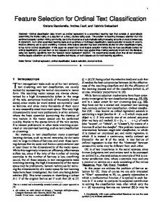
Figure 2: Diagram of a SDM, according to the original model, showing an array of bit counters to store data and an array of addresses. Memory locations within a certain radius of the reference address are selected to read or write. such a memory. Kanerva shows that the SDM naturally exhibits the properties of large boolean spaces. Those properties can be derived mathematically and are, to a great extent, similar to that of the human cerebellum. The SDM implements behaviours such as high tolerance to noise, operation with incomplete data, parallel processing and knowing that one knows.

3.1

Implementation of a SDM

The underlying idea behind the SDM is the mapping of a huge binary memory onto a smaller set of physical locations, so-called Hard Locations (HL). As a general guideline, those hard locations should be uniformly distributed in the virtual space, to mimic the existence of the larger virtual space as accurately as possible. Every datum is stored by distribution to a set of hard locations, and retrieved by sampling those locations. Figure 2 shows a model of a SDM. “Address” is the reference address where the datum is to be stored or read from. It will activate all the hard locations in a given access radius, which is predefined. Kanerva proposes that the Hamming distance, that is the number of bits in which two binary vectors are different, be used as the measure of distance between the addresses. All the locations that differ less than a predefined number of bits from the input address are selected (activated) for the read or write operation.

3.1.1

Writing and Reading

Data are stored in arrays of counters, one counter for every bit of every location. Writing is done by incrementing or decrementing the bit counters at the selected addresses. To store 0 at a given position, the corresponding counter is decremented. To store 1, it is incremented. The counters may, therefore, store either a positive or a negative value, which should, in theory, most of the times

WCE 2013

Proceedings of the World Congress on Engineering 2013 Vol II, WCE 2013, July 3 - 5, 2013, London, U.K.

fall into the interval [-40,40]. Reading is done by sampling the values of all the counters of all the active locations. A natural candidate to extract the correct value is the average. Summing all the counters columnwise and dividing by the number of active locations gives the average value of the counters. The average value can then be compared to a predefined threshold value. A threshold of 0 is appropriate for normal data—if the average value is below the threshold the bit to be read is zero, otherwise it is one. Figure 2 illustrates the method. But the average value is only one possible sampling method. Another possible method is to pool the information by taking a vote—the value that is the most popular among the contributing counters is preferred. Yet another alternative is to weigh the contribution of each counter based on the distance between each hard location and the reference address.

3.1.2

Starting the Memory

Initially, all the bit counters must be set to zero, for the memory stores no data. The bits of the hard locations’ addresses should be set randomly, so that those addresses would be uniformly distributed in the addressing space. However, many authors prefer to start with an empty memory, with neither data counters nor addresses, and then add more addresses where and when they are needed [6], in order to avoid processing unneeded locations and reduce startup time.

3.1.3

single pass. v) SDMs can be “open” and subject to analysis of individual locations. That is important namely for debugging purposes, or to track the learning process. vi) It is possible to change memory’s structure without retraining all the memory [6]. For example, it is possible to add locations where they are needed as well as remove unused locations. That is an important characteristic to build modular or adaptive systems. The main drawbacks of using Sparse Distributed Memories are: i) Once a datum is written, it cannot be erased, only forgotten as time goes by. Under certain circumstances that may be an undesirable feature. If unnecessary memories cannot be deleted, they may interfere with more recent and important data. ii) If the SDM is simulated in a common computer, storage capacity may be as low as 0.1 bits per bit of traditional computer memory, although many authors reported techniques to improve storage performance [9]. iii) If implemented in software, a lot of computer processing is required to run the memory alone.

3.2

Present implementation

In the present approach, the original SDM was implemented, with 8-bit counters (7 bits + sign). However, the hard locations were not placed randomly in the binary space as Kanerva proposes. The memory locations are managed using the Randomised Reallocation (RR) algorithm proposed by Ratitch et al. [6]. Using the RR, the system starts with an empty memory and allocates new locations when there is a new datum which cannot be stored into enough existing locations. The new locations are placed randomly in the neighbourhood of the new datum address.

Characteristics of the SDM

4 Due to the nature of the model, there is no guarantee that the data retrieved is exactly the same that was written. However, it is provable that under normal circumstances the hard locations must be correctly distributed over the binary space and, if the memory has not reached saturation, the correct data will be retrieved with high probability most of the times. The conclusion arises from the properties of high-dimensional boolean spaces. The mathematical details, due to their length, are out of the scope of this paper. They are elegantly described by Kanerva in [2]. A summary can also be found in [7]. Other important characteristics of the SDM are: i) It is immune to noise up to a high threshold. Using coding schemes such as n-of-m codes, the immunity is even increased [8, 5], at the cost of reducing the addressable space. ii) SDMs are robust to failure of individual locations, just like neural networks. iii) SDMs degrade gracefully, when some locations fail or the memory approaches its maximum capacity. iv) One-shot learning is possible. If the memory is not close to saturation, it will learn in a

ISBN: 978-988-19252-8-2 ISSN: 2078-0958 (Print); ISSN: 2078-0966 (Online)

Datasets

The datasets used in the experiments were pre-processed subsets of Reuters 21578 dataset, available from CardosoCachopo’s website1 [10]. Those datasets were chosen because of their popularity and the fact that they were available in pre-processed form from Cardoso-Cachopo’s website. The subset named R52 is a selection of documents which are classified into just one of the topics (singlelabelled). R52 contains 9100 documents distributed over 52 different topics. The subset named R8 is a selection of documents which are also single-labelled, but contains documents of just 8 of the 10 most frequent topics. Tables 1 and 2 show the number of documents per topic. As the tables show, data is very skewed, with the most popular class accounting for about half of the documents. Cardoso-Cachopo makes available the datasets with different pre-processing applied. The subsets that are relevant for the present experiments are: 1 Datasets

available at http://web.ist.utl.pt/acardoso/ (last checked 2013-02-10).

WCE 2013

Proceedings of the World Congress on Engineering 2013 Vol II, WCE 2013, July 3 - 5, 2013, London, U.K.

Table 1: Documents per class for dataset R8. Class Train set Test set Total 2292 acq 1596 696 crude 253 121 374 earn 2840 1083 3923 grain 41 10 51 interest 190 81 271 money-fx 206 87 293 ship 108 36 144 trade 251 75 326 Total 5485 2189 7674

• All-terms—Obtained from the original datasets by applying the following transformations: Substitute TAB, NEWLINE and RETURN characters by SPACE; Keep only letters (that is, turn punctuation, numbers, etc. into SPACES); Turn all letters to lower-case; Substitute multiple SPACES by a single SPACE; The title/subject of each document is simply added in the beginning of the document’s text. • Stemmed texts—Obtained from the previous file, by removing all words that are less than 3 characters long; removing the 524 SMART system’s stopwords2 and applying Porter’s Stemmer to the remaining words3 .

5

Experiments

To assess the performance of the SDM as a classifier, two types of vectors were used to represent the texts: TFIDF vectors and direct storage of the texts using ASCII characters. The experiments were performed in two steps: learning and testing. In the learning stage, representations of all the documents in the training sets were stored into the SDM. In the testing stage, the SDM was then queried with documents of the test set. The category of the document retrieved was then used as the SDM’s best match for the category of the test document. The first experiment was done using Term FrequencyInverse Document Frequency (TF-IDF) vectors as representations of the texts. TF-IDF is a popular statistic used to represent documents in text categorisation. In general, the use of TF-IDF vectors produces good results for text categorisation with popular methods such as Support Vector Machines, K-Nearest Neighbours and similar. In the present work, TF-IDF vectors were calculated for each single document in the train set. Those 2 ftp://ftp.cs.cornell.edu/pub/smart/english.stop (last checked 2013-02-13. 3 http://tartarus.org/∼martin/PorterStemmer/ (last checked 2013-02-13).

ISBN: 978-988-19252-8-2 ISSN: 2078-0958 (Print); ISSN: 2078-0966 (Online)

Table 2: Documents per class for dataset R52. Class Train set Test set Total 2292 acq 1596 696 alum 31 19 50 bop 22 9 31 carcass 6 5 11 cocoa 46 15 61 coffee 90 22 112 copper 31 13 44 cotton 15 9 24 cpi 54 17 71 cpu 3 1 4 crude 253 121 374 dlr 3 3 6 earn 2840 1083 3923 fuel 4 7 11 gas 10 8 18 gnp 58 15 73 gold 70 20 90 grain 41 10 51 heat 6 4 10 housing 15 2 17 income 7 4 11 instal-debt 5 1 6 interest 190 81 271 ipi 33 11 44 iron-steel 26 12 38 jet 2 1 3 jobs 37 12 49 lead 4 4 8 lei 11 3 14 livestock 13 5 18 lumber 7 4 11 meal-feed 6 1 7 money-fx 206 87 293 money-supply 123 28 151 nat-gas 24 12 36 nickel 3 1 4 orange 13 9 22 pet-chem 13 6 19 platinum 1 2 3 potato 2 3 5 reserves 37 12 49 retail 19 1 20 rubber 31 9 40 ship 108 36 144 strategic-metal 9 6 15 sugar 97 25 122 tea 2 3 5 tin 17 10 27 trade 251 75 326 veg-oil 19 11 30 wpi 14 9 23 zinc 8 5 13 Total 6532 2568 9100

WCE 2013

Proceedings of the World Congress on Engineering 2013 Vol II, WCE 2013, July 3 - 5, 2013, London, U.K.

vectors were then normalised and mapped in the interval [0, 127], so that all numbers could be represented as unsigned 7-bit integers. That conversion meant to loose a lot of precision, but considering the length of the vectors it was accepted as a good compromise between SDM simulation time and precision. In a second experiment, the vectors stored into the SDM were chunks of up to 8 Kb of the texts, coded in plain ASCII. When the length of the text was superior to 8 Kb, the text was truncated. When the length was inferior to 8 Kb, the remainder bytes were set at random. In both experiments, the encoded text was used as address for the SDM. The data stored was the text with the category juxtaposed—i.e., data vector was , where the category was always stored in plain ASCII text. During the learning stage, the vectors were stored into the SDM with a radius of zero. Copies of all vectors were stored, since all vectors were different from each other in both datasets. In the testing stage, the memory was queried with texts of the test set, encoded using the same method used during the learning stage. When plain texts were used, if the length of the test document was inferior to 8 Kb, only part of the vector was used to compute the similarity measure in the SDM. For example, if the length of the text was just 1 Kb, similarity was computed using only the first 1024 coordinates of the addresses of the hard locations. That should not affect the expected characteristics of the SDM, unless the text was too small.

6

Results

Table 3 summarises the results. The first column identifies the type of classifier. The second column shows the type of input used. The third column shows the results obtained for dataset R8 and the last one shows the results obtained for dataset R52. Experiments with other datasets and memory types were performed, but the performance of the SDM was very similar. Thus, for clarity, the authors chose to summarise the results into just Table 3. The “Dumb classifier” is shown just as a reference. It is a hypothetical classifier that always returns the most popular class. Thus, its performance is equal to the percentage of documents of the most popular class. In the datasets used, data is very skewed. Thus, the dumb classifier actually seems to have a good performance. In more homogeneous datasets the result is different. For example, in the “20 newsgroups dataset,” which consists of approximately 1000 messages of 20 different newsgroups (total close to 20000 messages), the dumb classifier has a performance of 5.3%, while the SDM achieves 20.94%

ISBN: 978-988-19252-8-2 ISSN: 2078-0958 (Print); ISSN: 2078-0966 (Online)

using “all-terms” and 22.17% using the stemmed texts. As for the SDM, two different methods were used for the prediction phase. First, the memory was configured in a way that for each prediction it always returned the nearest neighbour found in the neighbourhood of the input address. Second, the memory was configured in a way that it enlarged the access radius to encircle at least 10 data points, and then it returned the most popular class among the classes of data points found. Different numbers of data points were tested, between 2 and 10, and the differences were only negligible. In general, 10 seemed a good compromise. Using smaller numbers, the results tend to the results obtained in the first experiment. Enlarging the circle the results will tend to the performance of the dumb classifier. As Table 3 shows, the results obtained are humble if compared to other modern classifiers. For example, [11] reports an accuracy of up to 96.98% in dataset R8 and up to 93.77% in R52 using SVMs. However, the best results obtained with the SDM can be achieved naturally, with almost no text processing. The stemmed datasets apparently have a marginal improvement in the results. But even if the results are the same, stemming and removing stop-words contributes to reducing dimensionality of the input vectors. High-dimensionality is not a problem for the SDM, but if the SDM is implemented in common serial processors more dimensions mean more processing time. Thus, removing data that carries no useful semantic information speeds up the process without compromising accuracy. In summary, the results show that the SDM is able to grasp high-level semantic information from raw data input. There may be ways to improve the accuracy of the process, for example trying different methods of encoding the data. In some applications where real time processing is necessary, the SDM can still be a good option, even if the results are only humble compared to other modern methods. The results also open good perspectives for use of the SDM in other applications where text-matching is necessary, besides single-label text classification.

7

Conclusions

Text matching is a topic of increasing relevance, as it is important for information retrieval, text categorisation and other applications. It is known that language exhibits long-range correlations, from the lowest-level representations to the highest semantic meanings. The SDM is an associative memory model that works based on the properties of high-dimensional boolean spaces, exploring in part similarities between long binary vectors. The experimental results described in the present paper show that the original model of the SDM alone, without any text processing, is able to work as a surprisingly good text classifier, even taking plain ASCII text as input. In

WCE 2013

Proceedings of the World Congress on Engineering 2013 Vol II, WCE 2013, July 3 - 5, 2013, London, U.K.

Table 3: Performance of the classification methods compared. Method Input R8 R52 49.47 42.17 Dumb classifier TF-IDF vectors 55.92 51.01 SDM with shortest radius Stemmed texts 60.71 50.43 All terms 60.21 50.00 TF-IDF vectors 52.26 51.01 SDM choosing the most popular Stemmed texts 64.55 55.53 All terms 64.64 55.18

future work different methods of encoding the information or tuning the SDM may be tried, seeking to improve the performance of the SDM as a classifier.

References [1] Eduardo G. Altmanna, Giampaolo Cristadorob, and Mirko Degli Esposti. On the origin of long-range correlations in texts. Proceedings of the National Academy of Sciences of the United States of America, 109(29), 2012. [2] Pentti Kanerva. Sparse Distributed Memory. MIT Press, Cambridge, 1988.

[9] James D. Keeler. Comparison between Kanerva’s SDM and Hopfield-type neural networks. Cognitive Science, 12(3):299–329, 1988. [10] Ana Cardoso-Cachopo. Improving Methods for Single-label Text Categorization. PhD thesis, Universidade T´ecnica de Lisboa, October 2007. [11] Ana Cardoso-Cachopo and Arlindo Oliveira. Combining LSI with other classifiers to improve accuracy of single-label text categorization. In First European Workshop on Latent Semantic Analysis in Technology Enhanced Learning. EWLSATEL, 2007.

[3] David Rogers. Predicting weather using a genetic memory: A combination of Kanerva’s sparse distributed memory with Holland’s genetic algorithms. In NIPS, 1989. [4] Mateus Mendes, Manuel M. Cris´ostomo, and A. Paulo Coimbra. Robot navigation using a sparse distributed memory. In Proc. of IEEE Int. Conf. on Robotics and Automation, Pasadena, California, USA, May 2008. [5] Mateus Mendes, Manuel M. Cris´ostomo, and A. Paulo Coimbra. Assessing a sparse distributed memory using different encoding methods. In Proc. of the World Congress on Engineering (WCE), London, UK, July 2009. [6] Bohdana Ratitch and Doina Precup. Sparse distributed memories for on-line value-based reinforcement learning. In ECML, 2004. [7] Mateus Mendes, A. Paulo Coimbra, and Manuel Cris´ostomo. AI and memory: Studies towards equipping a robot with a sparse distributed memory. In Proceedings of the IEEE International Conference on Robotics and Biomimetics, pages 1743–1750, Sanya, China, December 2007. [8] Stephen B. Furber, John Bainbridge, J. Mike Cumpstey, and Steve Temple. Sparse distributed memory using n-of-m codes. Neural Networks, 17(10):1437– 1451, 2004.

ISBN: 978-988-19252-8-2 ISSN: 2078-0958 (Print); ISSN: 2078-0966 (Online)

WCE 2013