Exploring Non-Linear Relationships between Landscape and Aquatic ...

International Journal of Applied Geospatial Research, 5(4), 1-20, October-December 2014 1

Exploring Non-Linear Relationships between Landscape and Aquatic Ecological Condition in Southern Wisconsin: A GWR and ANN Approach

Richard R. Shaker, Department of Geography and Environmental Studies, Ryerson University, Toronto, Ontario, Canada Timothy J. Ehlinger, Department of Biological Sciences, University of Wisconsin, Milwaukee, WI, USA

ABSTRACT Recent studies have implied the importance of incorporating configuration metrics into landscape-aquatic ecological integrity research; however few have addressed the needs of spatial data while exploring nonlinear relationships. This study investigates spatial dependence of a measure of aquatic ecological condition at two basin scales, and the spatial and non-linear role of landscape in explaining that measure across 92 watersheds in Southern Wisconsin. It hypothesizes that: (1) indicators of ecological condition have different spatial needs at subwatershed and watershed scales; (2) land cover composition, urban configuration, and landscape diversity can explain aquatic ecological integrity differently; and (3) global non-linear analysis improve local spatial statistical techniques for explaining and interpreting landscape impacts on aquatic ecological integrity. Results revealed spatial autocorrelation in the measure of aquatic ecological condition at the HUC-12 subwatershed scale, and artificial neural networks (ANN) were an improvement over geographically weighted regression (GWR) for deciphering complex landscape-aquatic condition relationships. Keywords:

Fish Index of Biotic Integrity, Land Cover, Land Use Planning, Landscape Pattern, Multiple Regression Modeling, Spatial Analysis, Urbanization, Watershed Function

INTRODUCTION The current integrity of the planet is being stressed beyond its biological capacity, and

understanding human created landscapes is more important than ever. Changes in land cover, through the appropriation of natural landscapes to provide for human needs, has been found to

DOI: 10.4018/ijagr.2014100101 Copyright © 2014, IGI Global. Copying or distributing in print or electronic forms without written permission of IGI Global is prohibited.

2 International Journal of Applied Geospatial Research, 5(4), 1-20, October-December 2014

be one of the most pervasive alterations to native ecosystems resulting from human activity (Foley et al., 2005; Liu et al., 2007; Vitousek et al., 1997). Landscape change influences natural systems by fragmenting landscape patches, isolating habitats, abridging ecosystem dynamics, introducing exotic species, controlling and modifying disturbances, escalating climate change, and disrupting energy flow and nutrient cycling (Alberti, 2005; Alberti, 2008; Foley et al., 2005; Liu et al., 2007; Milly et al., 2008; Picket et al., 2001). Continuing with the impacts of landscape change, terrestrial waters are often those ecosystems most affected by associated stressors (Foley et al., 2005; Liu et al., 2007; Naiman & Turner, 2000; Novotny et al., 2005; Milly et al., 2008). Access and management of water resources is now considered a prerequisite for human development (Baron et al., 2002; Gleick, 2003). To support this, many nations throughout the world have adopted laws to protect or improve the integrity of hydrologic systems (Karr, 2006). A reoccurring theme throughout these regulations is to restore and maintain biological integrity of their respected waters. Monitoring programs for assessing human impacts on aquatic condition and water quality have existed for decades. Specifically, fish indicators of biological integrity have gained popularity for quantifying the impact of human activities on the biota and are in practice on six of the seven continents throughout the world (Roset et al., 2007). A variety of measuring techniques have been applied to fish as indicators of biological integrity; however, the Index of Biotic Integrity (IBI) has developed into the applied method of choice. The IBI (Karr, 1981) has been widely applied to fish assemblage data for assessing the environmental quality of aquatic habitats (Roset et al., 2007). Thus, the Fish Index of Biotic Integrity (F-IBI) has been welcomed as a robust method for investigating landscapeaquatic interactions (Karr & Yoder, 2004; Novotny et al., 2005), and has been found to help diagnose causes of ecological impacts and suggest appropriate management actions (Karr & Chu, 1999).

Previous studies between landscapeaquatic relationships have typically correlated changes in ecological integrity with simple aggregates of urbanization (e.g. percent urban) (Alberti et al., 2007). This paradigm has been reaffirmed since Klien’s (1979) seminal work with dozens of regional investigations on how land cover composition relates to aquatic conditions (e.g. Alberti et al., 2007; Morley & Karr, 2002; Roth et al., 1996; Richards et al., 1996; Shandas & Alberti, 2009; Thorne et al., 2000). With that said, these relationships are typically non-linear (Novotny et al., 2005), and by no means can account for all the variability in aquatic ecological integrity. Recently, studies have implied the importance of incorporating configuration metrics into landscape-aquatic condition research (e.g. Alberti et al., 2007; Shandas & Alberti, 2009). These studies provide much needed information to planners, natural resource managers, and landscape design specialists that cannot be addressed with simple aggregates of land cover (Alberti et al., 2007). Configuration studies quantify landscape fragmentation through spatially explicit metrics, and their results can help diagnose distributional effects of land use or land cover on ecosystem services (Shandas & Alberti, 2009). With that said, few configuration studies have fully addressed the needs of spatial data (e.g., spatial autocorrelation) in species-environment spatial analysis (King et al., 2005; Wagner & Fortin, 2005), and fewer have attempted to do so while exploring non-linear relationships with measures of in-stream ecological condition. When investigating species-environment relationships, it is important to take into account that many different processes influence natural systems over space. Two major quantitative shortcomings in spatial analysis of landscape-species interaction come from species patchiness, created by species-species relationships (e.g., competition), and by spatial dependence, created by species-environment relationships (e.g., niche habitat). Both forms of spatial structure are problematic in statistical analysis, as spatial autocorrelation in the residuals violates the assumption of independent

Copyright © 2014, IGI Global. Copying or distributing in print or electronic forms without written permission of IGI Global is prohibited.


observations and environmental heterogeneity restricts comparability of samples (Wagner & Fortin, 2005). Wagner and Fortin (2005) suggested using multiple regression spatial analysis, which allow for scrutinizing spatial autocorrelation of residuals, when modeling species-environment relationships. Traditional multiple regression techniques (e.g., OLS, ANOVA) have been commonly applied in landscape-aquatic condition research; however, these methods are problematic because they assume spatial stationarity in the relationships between variables under study (Legendre, 1993; Foody, 2003). Spatial non-stationarity and spatial autocorrelation are found commonly in environmental data (Legendre, 1993). A failure to account for spatial autocorrelation prevents an in-depth interpretation of almost all ecological studies over space (Boot, 2002; Jetz et al., 2004). Lennon (2000) called attention to these problems in ecological research and argued that virtually all geographic analyses had to be redone by taking into account spatial autocorrelation. This study investigates the spatial and non-linear role of landscape in explaining variations of aquatic ecological condition in Southern Wisconsin watersheds. Landscape is defined as both the amount of different land cover types, discrete mosaic of urban land cover, and landscape diversity. Building upon previous studies that examine relationships between composition and configuration of landscape and measures of aquatic ecological condition, we study this relationship using a spatially sensitive and non-linear methodology. Specifically, this research considers spatial and scale dependencies of an ecological condition indicator at two basin scales, and how the aforementioned landscape impacts that measure of in-stream biological conditions. To address these questions we test three null hypotheses: (1) no significant spatial dependence exists for mean F-IBI at both subwatershed and watershed aggregation scales; (2) no significant relationships exist between land cover composition, urban configuration, and landscape diversity with a measure of aquatic biological condition;

and (3) global non-linear analysis does not improve local spatial statistical techniques for explaining and interpreting landscape impacts on aquatic ecological integrity. By explicitly describing spatial dependencies of in-stream measures of ecological condition, and their non-linear relationships with basin composition and configuration, this research aims to improve scientific technique for understanding complex coupled landscape-aquatic relationships.

METHODS Study Area We have focused our biogeographical research in southern Wisconsin, USA (Figure 1). Several geographic characteristics make this region ideal for this study. The pre-settlement land cover for this area was largely prairie with small patches of woodlands and scattered wetlands throughout (Martin, 1965). The current predominant land cover and land use are agricultural and dairy farming, respectively. Further, this region of Wisconsin is historically known for its very fertile soils. A demographic shift to the hinterland has had a major influence on land use and land cover change, resulting in a variety of landscape patterns throughout the study area. Between 1970 and 2000, the population has increased by approximately 14 percent (USCB, 2000). The current landscape mosaic is primarily a result of suburban and exurban growth metabolizing and reshaping agricultural lands surrounding the two largest cities in the state: Madison and Milwaukee. Due to this urbanization, there was a loss of approximately 23 percent agricultural land from 1970 to 2000 (NASS, 2000). The surface geology is predominantly a result of the Wisconsin glacial recession with pockets of glacial till, lacustrine basins, and large areas of pitted and unpitted outwash plains (Dott & Attig, 2004). In the study area, elevation ranges from roughly 170 to 440 m above sea level. The study area spans four level III ecoregions; from west to east, these are: Driftless Area, North Central Hardwood Forests, Southeastern Wisconsin



Figure 1. Study area location within southern Wisconsin, USA displaying mean F-IBI across basin scales and urban land configuration (43°20’N, 89°29’W)

Till Plain, and Central Corn Belt Plains (see Omernik et al., 2000 for ecoregion details). Due to its agricultural legacy, this region has many floodplain alterations, including drainage tiling, channelizing, diking, and filling. Most of the streams and rivers within the study area have some type of hydrologic modification.

Watershed and Fish Index of Biotic Integrity (F-IBI) Data Numerous studies have demonstrated the importance of watershed scale research for improving aquatic and water quality over other management scales (e.g., reach, riparian zone) (Alberti et al., 2007; King et al., 2005; Potter et al., 2005; Roth et al., 1996; Wang et al., 2003; Wang et al., 2006). Starting in the mid 1970s, the watershed management paradigm changed

the way aquatic ecologists look at the landscape. “In every respect, the valley rules the stream” (Hynes, 1975). “Rivers and streams serve as a continent’s circulatory system, and the study of those rivers, like the study of blood, can diagnose the health not only of the rivers themselves but of their landscapes” (Sioli, 1975). Nested study area watersheds (HUC-10) and subwatersheds (HUC-12) were selected based on 715 fish sample sites, and an adjacent sampling of basins. HUC is the acronym for Hydrologic Unit Code and every hydrologic unit is uniquely identified through its code (2 to 12 digits) based on its scale within the hydrological system. The study area is comprised of 92 HUC-10 watersheds and 221 subwatersheds with varying shapes and sizes (Figure 1). Referred to as 5th level watersheds, the HUC-10 basins chosen in this analysis have



an average size of 350 km2 with a total study area of 32,200 km2. Referred to as the 6th level watersheds, the HUC-12 sub-basins employed in this analysis have an average size of 80 km2 with a total study area of 16,600 km2. USDA Forest Service published both the HUC-10 and HUC-12 basins selected in shapefile format in 2007. These data were digitized by interpreting USGS 7.5-minute, 1:24,000 scale topographic and hydrologic paper maps, elevation Digital Raster Graphics (DRGs), and digital orthophotos. For this study, the nested 92 watersheds and 221 subwatersheds should be considered as individual landscapes. The 715 fish sample sites used in this analysis are managed by the Wisconsin Department of Natural Resources (WDNR). Fish catch data collected over a span of four years (2001-2005) were used to calculate the F-IBI for each sample site; furthermore all F-IBI data and scores were collected and calculated by the WDNR. Due to geographical effects on speciation, the F-IBI employed is based on Lyons (1992) fish community research for the state of Wisconsin. Following the Wisconsin method for wadeable streams, fish samples are collected from a segment of stream with length equal to thirty-five times the mean stream width. This sampling methodology was designed to, and usually does, include different habitats (Karr et al., 1986; Lyons, 1992). The F-IBI for Wisconsin is calculated for an individual sample from each stream segment and calibrated by comparing the observed values of each metric with values expected in comparable streams of high environmental quality (Lyons, 1992). The Wisconsin F-IBI scales between 0 and 100, with increasing scores equaling improved environmental quality. For the 715 fish sample sites used, F-IBI scores range from 10 (very poor) to 50 (good). To reduce error from spatial autocorrelation of biotic processes (e.g., species interaction), spatial dependence from abiotic processes (e.g., deterministic structures such as canopy cover), and temporal variability, the aforementioned 715 F-IBI values were averaged to both HUC-10 and HUC-12 basin scales to create mean F-IBI (Figure 1).

Land Cover, Urban Configuration, and Landscape Diversity Data The 2001 (ver.2) land cover data used in this analysis were published by the Multi-Resolution Land Characteristics (MRLC) Consortium in 2010 as part of a National Land Cover Database (NLCD) for the conterminous United States. The MRLC is a partnership of Federal agencies led by the U.S. Geological Survey. The 2001 land cover data is a seamless 30-meter raster database of vegetation type, and was designed for an array of topics such as assessing ecosystem status and health, understanding spatial patterns of biodiversity, interpreting climate change, and developing land management policy. This database was created using dual-date Landsat Thematic Mapper (TM) imagery. NLCD 2001 for Wisconsin is organized into 16 land cover types; however for this analysis it has been reorganized into Anderson Level I classes (Anderson et al. 1976) land use and land cover classification system. For the conterminous United States, NLCD 2001 has an Anderson Level I class accuracy of 85.3 percent (Wickham et al., 2010). For our study area, there are seven applicable Anderson Level I classes. Composition of 2001 Anderson Level I classes was: agricultural land (39%), forest land (25%), rangeland (18%), urban or built-up (10%), and wetland (5%) for the 92 HUC-10 landscapes utilized in this study (percentages obtained from this analysis). Land cover (composition), urban patterns (configuration), and landscape diversity were quantified using landscape ecology metrics developed for quantifying the spatial arrangement of land cover and land use (McGarigal et al., 2002; Turner et al., 2001). FRAGSTATS version 3.4 (McGarigal et al., 2002), free and publicly accessible software, was used for computing land cover composition, urban pattern metrics, and diversity (heterogeneity) for each landscape (see Leitão et al., 2006). The reclassified land cover data preserved 30m resolution, and an 8-neighbor rule was selected for patch delineation. Five major land cover variables, 55 landscape urban class metrics, and two



Table 1. Geographically weighted regression bivariate results between landscape predictors and mean F-IBI. See Leitão et al. (2006) and McGarigal et al. (2002) for metric details

diversity measures were computed for each of the 92 HUC-10 watershed landscapes used in the following statistical analysis. As there is no causal ordering in space as there is in time, and there remains no minimum set of landscape metrics for capturing the majority of landscape structure (Wagner & Fortin, 2005), landscape measures were calculated and then statistically reduced into a highly relevant subset. Principal Components Analysis (PCA) and Robust Pearson correlations were used to reduce measures of landscape. Urban class metrics with strongest loadings that exhibited different patterns of orthogonal axes were selected. All remaining predictor variables were then reduced further by Robust Pearson correlations, to remove metrics that exhibited a high degree of multicollinearity (r > 0.75). Fourteen independent explanatory landscape variables remained to be used in the forthcoming univariate, bivariate, and multiple regression analyses (see Table 1). To meet the assumptions of normality for all variables required during

parametric tests, we used two types of transformation: negative arcsine (proportion data) and log10 (length/score data). The remaining landscape variables were standardized using a z-transformation to set all parameters to a mean of 0 and variance of 1. Other software packages implemented during this data processing step were: ESRI ArcGIS 10, SYSTAT 12, and JMP version 10 (SAS Institute, 2012).

Data Analysis A method is presented hereafter to assess relationships between landscape and aquatic ecological condition through the combination of traditional, spatial, and non-linear statistics. Specifically, exploratory spatial data analysis (ESDA), stepwise regression (OLS), geographically weighted regression (GWR), and artificial neural networks (ANN) were employed to test our hypotheses. In landscape-aquatic biological condition studies it is essential to take into account spatial autocorrelation. The first law of geography



states that things that are near are more similar (spatially autocorrelated) than things that are farther apart (Tobler, 1970). Spatial autocorrelation, the lack of independence between pairs of observation at given distances in time and space, is commonly found in environmental data (Legendre, 1993). In order to evaluate the spatial and scale dependencies of mean F-IBI at both basin scales, and independent variables of the bivariate and multiple regression analyses, an ESDA was conducted. For this study the common ESDA technique, spatial autocorrelation index global Moran’s I-test, was applied. Spatial autocorrelation index scores vary from each other; however, positive scores indicate similar values are spatially clustered and negative scores indicate unlike values are spatially clustered (Wong & Lee, 2005). ESDA is frequently used in studies of geographical ecology and macroecology (Dormann et al., 2007; Fortin & Dale, 2005; Lichstein et al., 2002; Wagner & Fortin, 2005; Rangel et al., 2010), and can be particularly useful when testing spatial autocorrelation in environmental systems. ESRI’s ArcMap 10 Spatial Statistics toolbox was employed to assess the level of spatial autocorrelation of variables used in this study. To ensure that every HUC basin had at least one neighbor, neighborhood definition for calculating Moran’s I scores was held constant at a Euclidean distance of 35 km. When investigating landscape-aquatic condition relationships it is essential to understand that many different processes influence natural systems over space. Traditionally, non-spatial multiple regression techniques (i.e., OLS) have been commonly applied in landscape-aquatic condition research; however, these methods are problematic because they assume spatial stationarity in the relationships between variables under study (Foody, 2003; Legendre, 1993). Spatial autocorrelation may be particularly problematic in regional-scale watershed studies because the locations of land cover patches are typically not uniformed over space and often correspond with the underlying foundation (e.g., geology, soils) of its landscape. Spatial autocorrelation has been found to be problematic

when investigating cause-effect relationships, because classical statistical tests (e.g., ANOVA) violate the assumption of independently distributed errors (Haining, 1990; Legendre, 1993). Further, standard errors are usually undervalued when positive autocorrelation is present and type I errors may be strongly exaggerated (Legendre, 1993), especially in association with changes in spatial scale (Hawkins et al., 2007). In most cases, the presence of spatial autocorrelation is seen as a significant shortcoming for hypothesis testing and prediction (Dormann et al., 2007; Lennon, 2000). To date, there remain few statistical methods that consider non-stationarity across an entire region of study (Osborne et al., 2007). In landscape-aquatic biological condition research, this phenomenon is occasionally acknowledged and rarely addressed quantitatively (King et al., 2005). GWR, a refinement to traditional regression methods, utilizes a distance decay weighted philosophy that explicitly deals with the spatial non-stationarity of empirical relationships (Fotheringham et al., 2002; Fotheringham, 2004; LeSage, 1999;). GWR assesses local influences, allowing for a spatial shift in parameters and a more appropriate model fit (Wang et al., 2005). Thus, GWR models are not designed for extrapolation beyond the region in which they were established; however they may be more suitable for descriptive and predictive purposes (Foody, 2003). Using GWR as an exploratory tool, relationships between mean F-IBI and the fourteen landscape variables were measured. GWR was undertaken using a Bi-Square spatial weighting with optimization for minimizing corrected Akaike Information Criterion (AICc). For variable evaluation, AICc was applied as a preferred measure of model fit (see Akaike, 1978; Fotheringham et al., 2002). In general, the lower the AICc the closer the approximation of the model is to reality; however a ‘serious’ difference between two models is when the difference in AICc values differ by at least three (Fotheringham et al., 2002). Spatial Analysis in Macroecology (SAM) version 4, software specifically developed to address spatial data needs found naturally in



macroecological and biodiversity data (Rangel et al., 2010), was used to calculate and interpret all GWR models. Statistically significant landscape predictors from the bivariate GWR analysis were reduced to those that correlated with mean F-IBI using a multiple regression exploratory technique. This statistical procedure for model development used a forward stepwise regression method (P-value = 0.05 to remove). A multiple regression landscape model explaining mean FIBI was created to test our hypotheses. Using a Bi-Square spatial weighting with optimization for minimizing AICc, SAM version 4 was used to calculate and interpret the multiple regression GWR model. In multiple regression models, the dominant practice is to rank the standard partial regression coefficients (Sokal & Rohlf, 1995) or associated t-values of coefficients of explanatory variables (Tognelli & Kelt, 2004) under the assumption that higher coefficients represent stronger “effects” on the dependent variable (Bini et al., 2009). To measure the impact of multicollinearity we estimated the variance inflation factor (VIF). VIF > 10 indicates definite problems of multicollinearity; VIF > 2.5 indicates potential areas of concern. Many factors can influence measures of aquatic ecological integrity, many factors of which cannot be quantified accurately. Further, coupled human-environmental systems are often non-linear (Legendre & Legendre 1998; Novotny et al., 2005), and understanding those relationships can provide knowledge germane to understanding thresholds of landscape effects. ANN has gained popularity in the natural sciences to help describe complex and non-linear relationships between environmental processes (e.g., May et al., 2008; Salazar-Ruiz et al., 2008; Shaker et al., 2010). ANN is a data-driven computation technique that was originally inspired by neurobiology brain function of study, memory, reasoning, and induction (Beale & Jackson, 1998). ANN is especially useful for offering solutions by learning and adapting to difficult to understand, incomplete, noisy, and fuzzy information (Fisher & Abrahart, 2000);

albeit, ANN’s ability to learn and adapt is considered one of its most important characteristics (Beale & Jackson, 1998; Graupe, 2007). ANN has also been found to be particularly useful in studies with data shortcomings (Fischer & Abrahart, 2000; Openshaw 1998; Shaker et al., 2010). ANN operates by creating connections between processing elements (analogous to neurons in the brain). Each processing element takes many input signals, then, based on an internal weighting system, produce output signals that are sent as inputs to the other processing elements (Porwal et al., 2003). The network weights are modified in a training process through a number of learning algorithms based on back propagation learning (Brown et al., 2003). During the learning process, it is imperative that the training and validation sets are representative of the same population. A typical feed-forward ANN consists of three layers- input processing elements, hidden layers, and output. The number of input processing elements (neurons) is equal to the data variables used. The number of hidden layers depends on the architecture of the network and is usually determined by trial and error (Samanta et al., 2006). In recent landscape studies, progress has been made on ANN architecture, circumventing vagueness (see Lakes et al., 2009; Pijanowski et al., 2002; Pijanowski et al., 2005). A frequently used ANN procedure is the k-fold cross-validation method (e.g, Shaker et al., 2010). In this case, the dataset is equally divided into k parts and fits data repeatedly k times on overlapping (k-1)/k proportions of the data. However, it is optimal if two independent databases are used (Lek & Gue´gan, 1999), one for training and one for validating the model (e.g., Obach et al., 2001). Shaker et al. (2010) recently used ANN to decipher the complex relationships between the landscape mosaic and a measure of groundwater quality. That study suggests that ANN can also provide an effective addendum to modeling the complex non-linear relationships found in coupled landscape-aquatic condition research.



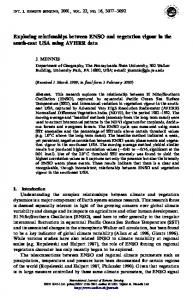
Figure 2. Structure of urban landscape artificial neural network for predicting mean F-IBI

To date, application of ANN for investigating relationships between landscape and measures of ecological condition are still limited. Using the statistical software JMP version 10 (SAS Institute, 2012), a randomized training (n = 74)/ validation (n = 18) feedforward ANN model was incorporated into this study for interpreting the non-linear relationships between landscape and mean F-IBI. A standard weighted-decaystabilized Gauss Newton estimation method was used to train the neural network (Bishop, 1995). The structure of our urban landscape ANN model for predicting mean F-IBI comprised of four input variables, three hidden nodes, and one output variable (Figure 2). For this analysis, the S-shaped activation function (S(x)= 1/(1+e-x)), overfit penalty (0.01), number of tours (16), and converge criterion (0.00001) were all kept at default in JMP software version 10 (SAS Institute, 2012).

RESULTS Exploratory Spatial Data Analysis Investigating spatial and scale dependencies of mean F-IBI at both basin scales revealed a high degree of spatial autocorrelation at the subwatershed scale. Global Moran’s I index reported a score of 0.19, z-score = 5.11 for mean F-IBI at the HUC-12 sub-basin scale, thus signifying that there is less than 1% likelihood that this spatial pattern could be the result of random chance. At the HUC-10 basin scale, Global Moran’s I reported mean F-IBI to be spatially random with an index score of 0.02, z-score = 0.51. Due to spatial dependencies of our fish indicator of aquatic integrity at the HUC-12 subwatershed scale, the subsequent analysis and results are from the HUC-10 watershed scale. No spatial autocorrelation was revealed in either the dependent or independent variables of the landscape model (Table 2).



Table 2. Multicollinearity results of independent covariates, and spatial autocorrelation findings for all variables used in urban landscape model

GWR Bivariate Analysis GWR captured the bivariate spatial relationships between major land cover composition, urban configuration, and landscape diversity with mean F-IBI at the HUC-10 basin scale (Table 1). The results of this investigation suggest that urban pattern measures are more important than landscape composition for predicting indicators of in-stream biological integrity. Of the fourteen landscape-aquatic condition relationships tested, eleven independent landscape predictors were statistically significant; two were composition metrics, two were landscape diversity measures, and seven were urban class configuration metrics. Overall, the best land cover composition predictor of mean F-IBI was percent urban/built-up (% Urban) (AICc = 624.18, R2 = 0.49). Shannon’s diversity index (SHDI), a popular ecological diversity index based on information theory (McGarigal et al., 2002), was the best landscape diversity measure at explaining mean F-IBI (AICc = 653.26, R2 = 0.36). The best urban class configuration metric for explaining mean F-IBI was area-weighted mean Euclidean nearest-neighbor distance (ENN_AM) (AICc = 617.93, R2 = 0.59). ENN_AM is the sum, across all urban patches in a HUC-10 landscape, of the nearest neighbor distance of each urban patch multiplied by the proportional abundance of the patch (Leitão et al., 2006). Of the seven statistically significant urban class configuration metrics, one is an

area measure, one is an isolation measure, two are aggregation measures, and three are shape measures (McGarigal et al., 2002). Testing residual spatial dependence of each bivariate model, using Global Moran’s I index, revealed no spatial errors.

Multiple Regression Analyses The stepwise exploratory analysis eliminated seven of the remaining eleven landscape variables from the preceding GWR analysis. The remaining four variables combined to make a multiple regression urban landscape model for explaining mean F-IBI. The model consists of one land cover composition measure and three urban class configuration metrics (Table 3A). The one land cover composition measure was: percent urban/built-up land (% Urban). The three urban class configuration metrics were: area-weighted mean Euclidean nearest-neighbor distance (ENN_AM), range of fractal dimension index (FRAC_RA), and mean radius of gyration (GYRATE_MN). As VIF magnitudes in Table 2 are between 1.10 and 1.98, the risk of collinearity among the urban landscape model covariates is very low to nonexistent. Based on OLS methodology, the four aforementioned landscape predictors combined to explain 37 percent of the variation in mean F-IBI (R2 = 0.37, P < 0.001), across 92 Southern Wisconsin HUC-10 landscapes (Table 3B).



Table 3. Results of stepwise multiple regression for mean F-IBI as a function of urban landscape composition and configuration. Final regression model showing standardized coefficients (A); analysis of variance (B); and overall significance (C)

Based on the OLS urban landscape model, the strongest positive influence of an individual predictor for explaining mean F-IBI was areaweighted mean Euclidean nearest-neighbor distance (ENN_AM, std. coeff. = 0.26, P = 0.02, Table 3A). Based on the OLS urban landscape model, the strongest negative influence of an individual predictor for explaining mean F-IBI was percent urban/built-up land (% Urban,

std. coeff. = -0.26, P = 0.031, Table 3A). As landscape-aquatic relationships are inherently spatial, GWR multiple regression methodology proved to be an enhancement over OLS (Table 3B). The GWR urban landscape model, with the four aforementioned landscape covariates, combined to explain 53 percent of the variation in mean F-IBI (R2 = 0.53, P < 0.001), across 92 Southern Wisconsin HUC-10 landscapes



Figure 3. Actual versus predicted plot of mean F-IBI score from GWR model (A); and frequency distribution of GWR model residuals (B)

(Table 3C, Figure 3A). Investigating spatial autocorrelation of the urban landscape model further, autocorrelation has been avoided during the multiple regression GWR analysis based on a normal distribution of model residuals (Figure 3B). Significant non-linear relationships were found between urban landscape predictors and the indicator of aquatic ecological condition. The resulting ANN model supported OLS and GWR urban landscape multiple regression models for predicting mean F-IBI. The three nodes captured variation in aquatic condition differently, and significant non-linearity of the relationships between landscape and mean FIBI (Table 4). Based on ANN methodology, the urban landscape model combined to explain 51 percent of the variation of mean F-IBI across 74 Wisconsin HUC-10 landscapes during the training process (R2 = 0.51, P < 0.001), and 56 percent of the variation across 18 Wisconsin

HUC-10 landscapes during the validation process (R2 = 0.56, P < 0.001) (Figure 4). The non-linear relationships found in this analysis provide the opportunity to inspect thresholds of landscape effects on indicators of aquatic ecological integrity.

DISCUSSION When using IBI as an indication of ecological condition, it is important to take into consideration the natural variability that remains in the index, which could hamper its sensitivity to human disturbance (Roset et al., 2007). Although the rationale behind the IBI is strongly supported, and methods have been continuously improved for wider application (Karr and Chu, 1999), some landscape-aquatic condition studies may have failed to address certain spatial relationships. Sampling design of the IBI, and its incorporation into landscape studies, may



Table 4. Parameter estimates for the three hidden nodes of the urban landscape artificial neural network model predicting mean F-IBI

induce quantitative shortcoming in spatial analysis. Specifically, IBI sampling methodology was designed to include different habitats (Karr et al., 1986; Lyons, 1992); however, if sample sites do not have heterogeneity in their reach’s habitat, species-environmental dependence exists restricting comparability in samples (Wagner & Fortin, 2005). This phenomenon in landscape-aquatic research could be especially problematic when one IBI sample site is correlated to a large area of study (e.g., watershed). In another aspect of landscape-species spatial analysis, species

patchiness may occur if aggregation units are smaller than the indicator species’ range. By having species-species interaction, Type I error is created through the lack of independent observations. In species-environment research, this phenomenon is avoided by adopting artificial randomness into statistical design, thus creating independent observations. However, by doing so, a mismatch between species response and ideal management scale could occur. In this study, measures were taken to elevate possible spatial data shortcoming of F-IBI as a response variable; thus, allowing for better un-

Figure 4. Actual versus predicted plot of mean F-IBI for training and validating urban landscape artificial neural network model



derstanding of spatial and scale dependencies of fishes in landscape-aquatic condition research. Trying to circumvent species-environmental dependencies, 715 F-IBI sample sites from different years and seasons were averaged to 92 HUC-10 watersheds and 221 HUC-12 subwatersheds. By creating mean F-IBI, errors associated with spatial autocorrelation of biotic and abiotic processes, and temporal variability were reduced. To investigate species-species interaction and dependencies, and its relevance to ideal management scale (e.g. HUC scale) for landscape analysis, spatial autocorrelation index global Moran’s I-test was applied. Our exploratory spatial data analysis of mean FIBI at both HUC-10 and HUC-12 basin scales revealed highly significant species-species interdependence at the HUC-12 subwatershed aggregation scale and spatial randomness at the HUC-10 watershed aggregation scale. This research suggests, when using fish as indicators of aquatic biological condition, landscape analyses should be conducted at the HUC-10 watershed scale to avoid spatial dependencies or an autoregressive methodology should be adopted at the HUC-12 subwatershed scale. The results of both the GWR and ANN analyses clearly show an improvement over linear (e.g. OLS) methods for understanding landscape-aquatic ecological relationships. Over the past decades, numerous studies have linked landscape composition with aquatic ecosystem condition (e.g., Booth et al., 2002). Historically, broad measures of urbanization have emerged as perhaps the most prominent stressor, but it is now clear that there is no single best variable that explains complex relationships between urban landscapes and aquatic ecological condition in watersheds. As aquatic ecosystems can be altered by human actions in several ways (Karr, 1999), and strong correlation between measures of urban development and IBI have been previously found (e.g., Morely & Karr, 2002), our study confirms that multiple regression non-linear approaches elucidate these relationships further. More recently, studies between landscape and aquatic condition in watersheds have improved

results by incorporating land cover configuration metrics (e.g., Alberti et al., 2007; Shandas & Alberti, 2009). As aggregates of land cover (e.g., percent urban) provide limited landscape design/structure results, configuration metrics provide much needed insight to environmental planners, natural resource managers, and landscape design specialists. Our study confirms the strong correlation between land cover configuration and IBI, and adds that multiple regression non-linear methods improve the understanding of these relationships. The response profile of our ANN urban landscape model (Figure 5) provides a visual narrative on how landscape composition and configuration relates to mean F-IBI non-linearly. As in other studies, our research finds a negative logarithmic relationship between percent urban/built-up land (% Urban) and mean F-IBI. As watersheds increase their urban composition, aquatic ecological condition deteriorates exponentially. Area-weighted mean Euclidean nearest-neighbor distance (ENN_AM) and range of fractal dimension index (FRAC_RA) have relatively linear positive relationships with mean F-IBI. ENN_AM is perhaps one of the simplest measures of urban patch isolation, equals the average Euclidean distance of nearest urban patch neighbor, and increases without limit (McGarigal et al., 2002). In our study, this relationship is interpreted as urban patches are placed farther apart from each other in space there will be improved aquatic ecological condition. FRAC_RA reflects shape complexity across a range of urban patch sizes; albeit, index scores range between one and two with one representing simple perimeters (e.g., square) and two representing complex (e.g., convoluted) perimeters (McGarigal et al., 2002). In this study, these results suggest that, as urban patches deviate from simple shape geometry, aquatic ecological condition is improved. GYRATE_MN is the average urban patch area within a landscape, its values increases without limit, and achieves maximum score when the urban patch comprises the entire watershed (McGarigal et al., 2002). Mean F-IBI shows no response to Mean radius of gyration



Figure 5. Response profile of artificial neural network model predicting mean F-IBI

(GYRATE_MN) until a threshold is reached which causes a negative relationship until another threshold is reached causing a slight positive relationship. Since the first threshold is around the mean, we find that urban patch size increase does not negatively impact aquatic ecological condition until GYRATE_MN scores roughly equal 149 (Min = 98.84, Mean = 149.33, Max = 196.67). Unfortunately, due to transformation and standardization of independent variables, we cannot interpret the level where GYRATE_MN at a larger area starts to positively impact mean F-IBI. Detailed threshold of effect information of urban configuration would improve watershed management policies that presently lack any such regulatory limits.

CONCLUSIONS Processes related to urbanization and traditional economic development are linked to ecological degradation, however they are by no means homogenous or uniform in terms of their explicit spatial patterns or detailed impacts to biological function (Alberti et al., 2007). By building on existing land cover/land use composition and configuration studies on measure of aquatic ecological integrity, this research examines the role landscape has on mean F-IBI spatially and non-linearly. Although attempts were made to circumvent spatial autocorrelation by averaging 715 fish sample sites to 92 HUC-10 watersheds

and 221 HUC-12 subwatersheds, our results revealed species-species dependence at the HUC-12 scale. Thus, the first null hypothesis is accepted because spatial autocorrelation index global Moran’s I-test revealed statistically significant results of mean F-IBI at the HUC-12 aggregation scale. The subsequent bivariate and multiple regression analyses identified land cover composition, urban configuration, and landscape diversity are relevant to predicting aquatic ecological integrity across 92 HUC-10 watersheds in Southern Wisconsin. The second null hypothesis stated that no significant relationships exist between land cover composition, urban configuration, and landscape diversity with a measure of aquatic biological condition. As at least one predictor representing landscape composition, urban configuration, and landscape diversity was statistically significant at explaining mean F-IBI during the bivariate GWR analysis, the second null hypothesis is rejected. This study provides empirical evidence for utilizing spatial and non-linear methods for explaining landscape-aquatic biological condition relationships. The third and final null hypothesis stated global non-linear analysis does not improve local spatial statistical techniques for explaining and interpreting landscape impacts on aquatic ecological integrity. In agreement with current literature, GWR and ANN enhanced the urban landscape model Coefficient of Determination



by explaining 16 and 19 (validation) percent more of mean F-IBI variation, respectively than OLS. The global non-linear analysis employed had a three percent Coefficient of Determination improvement over the local spatial statistical method. The ANN response profile proved to be a superior tool over GWR outputs for interpreting non-linear relationships between landscape and ecological condition. With these combined results, the third and final hypothesis is also rejected. By explicitly describing spatial dependencies of in-stream measures of ecological condition, and their non-linear relationships with basin composition and configuration, this research provides scientific technique for further understanding complex coupled landscapeaquatic relationships. Collectively, our results reveal that watersheds with urban patches that are disaggregated (away from each other in space), convoluted (irregularly shaped), and have area less than a specific threshold, will have improved aquatic ecological condition. While this study across watersheds in Southern Wisconsin provides a spatially sensitive and non-linear method for exploring how landscape influences ecological conditions, caution must be applied when trying to transfer results and much remains to be explored. More research could be pursued to address specific threshold of effects caused by landscape change. While this paper confirms that landscape does explain a great deal of aquatic ecological condition, there are multiple mechanisms operating simultaneously in watersheds and more research is needed to understand these complex coupled systems. By exploring spatial and non-linear landscape-aquatic condition relationships further, watershed planning practices and policy can be improved at local and regional scales. In final, knowledge from studies like these help determine processes that need to be modified or maintained to ensure the future of global systems.

ACKNOWLEDGMENT The research and modeling analyses contained within this article were sponsored by the United States Environmental Protection Agency/ National Science Foundation/United States Department of Agriculture STAR Watershed Program (Grant No. R83-0885-010). Additional support was provided by the Wisconsin Department of Natural Resources (WDNR). The findings and conclusions of this article are those of the authors and not to reflect on the aforementioned agencies.

REFERENCES Akaike, H. (1978). A Bayesian analysis of the minimum AIC procedure. Annals of the Institute of Mathematical Statistics A, 30(1), 9–14. doi:10.1007/ BF02480194 Alberti, M. (2005). The effects of urban patterns on ecosystem function. International Regional Science Review, 28(2), 168–192. doi:10.1177/0160017605275160 Alberti, M. (2008). Advances in urban ecology: integrating humans and ecological processes in urbanecosystems. New York: Springer. doi:10.1007/9780-387-75510-6 Alberti, M., Booth, D., Hill, K., Coburn, B., Avolio, C., Coe, S., & Spirandelli, D. (2007). The impacts of urban pattern on aquatic ecosystems: An empirical analysis in Puget lowland sub-basins. Landscape and Urban Planning, 80(4), 345–361. doi:10.1016/j. landurbplan.2006.08.001 Anderson, J. R., Hardy, E. E., Roach, J. T., & Witmer, R. E. (1976). A land use and land cover classification system for use with remote sensor data. Geological Survey Professional Paper 964. Washington: United States Government Printing Office. Baron, J. S., Poff, N. L., Angermeier, P. L., Dahm, C. N., Gleick, P. H., & Hairston, N. G. et al. (2002). Balancing human and ecological needs for freshwater: The case for equity. Ecological Applications, 12, 1247–1260. doi:10.1890/10510761(2002)012[1247:MEASNF]2.0.CO;2 Beale, R., & Jackson, T. (1998). Neural computing: An introduction. Institute of Physics Publishing.



Bini, L. M., Diniz-Filho, A. F., Rangel, T. F. L. V. B., Akre, T. S. B., Albaladejo, R. G., & Albuquerque, F. S. et al. (2009). Coefficient shifts in geographical ecology: An empirical evaluation of spatial and non-spatial regression. Ecography, 32(2), 193–204. doi:10.1111/j.1600-0587.2009.05717.x Bishop, C. M. (1995). Neural networks for pattern recognition. Oxford University Press. Booth, D. B., Hartley, D., & Jackson, R. (2002). Forest cover, impervious-surface area, and the mitigation of stormwater impacts. Am. Water Resources Assoc., 38(3), 853–845. Boots, B. (2002). Local measures of spatial association. Ecoscience, 9, 168–176. Brown, W., Groves, D., & Gedeon, T. (2003). Use of fuzzy membership input layers to combine subjective geological knowledge and empirical data in a neural network method for mineral-potential mapping. Natural Resources Research, 12(3), 183–200. doi:10.1023/A:1025175904545 Dormann, C. F., McPherson, J. M., Araújo, M. B., Bivand, R., Bolliger, J., & Carl, G. et al. (2007). Methods to account for spatial autocorrelation in the analysis of species distributional data: A review. Ecography, 30, 609–628. doi:10.1111/j.2007.09067590.05171.x Dott, R. H., & Attig, J. W. (2004). Roadside geology of Wisconsin. Madison, Wi: University of Wisconsin Press. ESRI ArcGIS 10. (1999-2012). Computer Software, Redlands, CA. Fischer, M. M., & Abrahart, R. J. (2000). Neurocomputing - Tools for Geographers. In S. Openshaw, & R. J. Abrahart (Eds.), GeoComputation (pp. 187–217). New York: Taylor & Francis. Foley, J. A., DeFries, R., Asner, G. P., Barford, C., Gordon, B., & Carpenter, S. R. et al. (2005). Global consequences of land use. Science, 309(5734), 570– 574. doi:10.1126/science.1111772 PMID:16040698 Foody, G. M. (2003). Geographical weighting as a further refinement to regression modelling: An example focused on the NDVI-rainfall relationship. Remote Sensing of Environment, 88(3), 283–293. doi:10.1016/j.rse.2003.08.004 Fortin, M. J., & Dale, M. R. T. (2005). Spatial analysis: a guide for ecologists. Cambridge, United Kingdom: Cambridge University Press.

Fotheringham, A. S., Brundson, C., & Charlton, M. E. (2004). Quantitative geography. London: Sage Publications. Fotheringham, A. S., Brunsdon, C., & Charlton, M. E. (2002). Geographically weighted regression: the analysis of spatially varying relationships. Chichester: Wiley. Gleick, P. H. (2003). Global freshwater resources: Soft-path solutions for the 21st century. Science, 302(5650), 1524–1528. doi:10.1126/science.1089967 PMID:14645837 Graupe, D. (2007). Principles of artificial neural networks. 2nd Ed. Advanced series of circuits and systems. World Scientific Publishing Co: Singapore. Haining, R. (1990). Spatial data analysis in the social and environmental sciences. Cambridge, United Kingdom: Cambridge University Press. doi:10.1017/ CBO9780511623356 Hynes, H. B. N. (1975). The stream and its valley. Verhandlungen - Internationale Vereinigung für Theoretische und Angewandte Limnologie, 19, 1–15. Jetz, W., Carbone, C., Fulford, J., & Brown, J. H. (2004). The scaling of animal space use. Science, 306(5694), 266–268. doi:10.1126/science.1102138 PMID:15472074 Karr, J. R. (1981). Assessment of biotic integrity using fish communities. Fisheries (Bethesda, Md.), 6(6), 21–27. doi:10.1577/1548-8446(1981)0062.0.CO;2 Karr, J. R. (2006). Seven foundations of biological monitoring and assessment. Biologia Ambientale, 20, 7–18. Karr, J. R., & Chu, E. W. (1999). Restoring life in running waters: better biological monitoring. Washington, DC: Island Press. Karr, J. R., Fausch, K. D., Angermeier, P. L., Yant, P. R., & Schlosser, I. J. (1986). Assessing biological integrity in running waters: a method and its rationale (Vol. 5). Champaign, IL: Illinois Natural Survey Special Publication. Karr, J. R., & Yoder, C. O. (2004). Biological assessment and criteria improve TMDL decision making. Journal of Environmental Engineering, 130, 594–604. doi:10.1061/(ASCE)07339372(2004)130:6(594)



King, R. S., Baker, M. E., Whigham, D. F., Weller, D. E., Jordan, T. E., Kazyak, P. F., & Hurd, M. K. (2005). Spatial considerations for linking watershed land cover to ecological indicators in streams. Ecological Applications, 15(1), 137–153. doi:10.1890/04-0481 Klien, R. D. (1979). Urbanization and stream quality impairment. Journal of the American Water Resources Association, 15, 1211–1219. Lakes, T., Müller, D., & Krüger, C. (2009). Cropland change in southern Romania: A comparison of logistic regressions and artificial neural networks. Landscape Ecology, 24(9), 1195–1206. doi:10.1007/ s10980-009-9404-2 Legendre, P. (1993). Spatial autocorrelation: Trouble or new paradigm? Ecology, 74(6), 1659–1673. doi:10.2307/1939924 Legendre, P., & Legendre, L. (1998). Numerical ecology (2nd ed.). Elsevier. Leitão, A. B., Miller, J., Ahern, J., & McGarigal, K. (2006). Measuring landscapes: a planner’s handbook. Washington, DC, USA: Island Press. Lek, S., & Gue’gan, J. F. (1999). Artificial neural networks as a tool in ecological modelling, an introduction. Ecological Modelling, 120(2-3), 65–73. doi:10.1016/S0304-3800(99)00092-7 Lennon, J. J. (2000). Red-shifts and red herrings in geographical ecology. Ecography, 23(1), 101–113. doi:10.1111/j.1600-0587.2000.tb00265.x LeSage, J. P. (1999). A family of geographically weighted regression models. Regional Science Association International Meetings. doi:10.1007/9783-662-05617-2_11 Lichstein, J. W., Simons, T. R., Shriner, S. A., & Franzreb, K. E. (2002). Spatial autocorrelation and autoregressive models in ecology. Ecological Monographs, 72(3), 445–463. doi:10.1890/00129615(2002)072[0445:SAAAMI]2.0.CO;2 Liu, J., Dietz, T., Carpenter, S. R., Alberti, M., Folke, C., & Moran, E. et al. (2007). Complexity of coupled human and natural systems. Science, 317(5844), 1513–1516. doi:10.1126/science.1144004 PMID:17872436 Lyons, J. (1992). Using the Index of Biotic Integrity (IBI) to measure environmental quality in warmwater streams of Wisconsin. General Technical Report: NC149, US Department of Agriculture, Washington, DC. Martin, L. (1965). The physical geography of Wisconsin. Madison, Wi: University of Wisconsin Press.

May, R. J., Maier, H. R., Dandy, G. D., & Fernando, T. M. K. G. (2008). Nonlinear variable selection for artificial neural networks using particle mutual information. Environmental Modelling & Software, 23(10–11), 1312–1326. doi:10.1016/j. envsoft.2008.03.007 McGarigal, K., Cushman, S. A., Neel, M. C., & Ene, E. (2002). FRAGSTATS: spatial pattern analysis program for categorical maps. Computer software program produced by the authors at the University of Massachusetts, Amherst. Available at the following web site: http://www.umass.edu/landeco/research/ fragstats/fragstats Milly, P. C. D., Betancourt, J., Falkenmark, M., Hirsch, R. M., Kundzewicz, Z. W., Lettenmaier, D. P., & Stouffer, R. J. (2008). Stationarity is dead: Whither water management? Science, 319(5863), 573–574. doi:10.1126/science.1151915 PMID:18239110 Morley, S. A., & Karr, J. R. (2002). Assessing and restoring the health of urban streams in the Puget Sound Basin. Conservation Biology, 16(6), 1498–1509. doi:10.1046/j.1523-1739.2002.01067.x Naiman, R. J., & Turner, M. G. (2000). A future perspective on North America’s freshwater ecosystem. Ecological Applications, 10(4), 958–970. doi:10.1890/1051-0761(2000)010[0958:AFPON A]2.0.CO;2 NASS – National Agricultural Statistics Service. (2000). Retrieved on 6 January 2007 from http:// www.nass.usda.gov/Statistics_by_State/Wisconsin/ index.asp Novotny, V., Bartošová, A., O’Reilly, N., & Ehlinger, T. J. (2005). Unlocking the relationship of biotic integrity of impaired waters to anthropogenic stresses. Water Research, 39(1), 184–198. doi:10.1016/j. watres.2004.09.002 PMID:15607177 Obach, M., Wagner, R., Werner, H., & Schmidt, H. H. (2001). Modelling population dynamics of aquatic insects with artificial neural networks. Ecological Modelling, 146(1-3), 207–217. doi:10.1016/S03043800(01)00307-6 Omernik, J. M., Chapman, S. S., Lillie, R. A., & Dumke, R. T. (2000). Ecoregions of Wisconsin. Transactions of the Wisconsin Academy of Sciences, Arts, and Letters, 88, 77–103. Openshaw, S. (1998). Neural network, genetic, and fuzzy logic models of spatial interaction. Environment & Planning A, 30(10), 1857–1872. doi:10.1068/ a301857



Osborne, P. E., Foody, G. M., & Suárez-Seoane, S. (2007). Non-stationarity and local approaches to modelling the distributions of wildlife. Diversity & Distributions, 13(3), 313–323. doi:10.1111/j.14724642.2007.00344.x Picket, S. T. A., Cadenasso, M. L., Grove, J. M., Nilon, C. H., Pouyat, R. V., Zipperer, W. C., & Costanza, R. (2001). Urban ecological systems: Linking terrestrial ecology, physical, and socioeconomic components of metropolitan areas. Annual Review of Ecology and Systematics, 32(1), 127–157. doi:10.1146/annurev. ecolsys.32.081501.114012 Pijanowski, B. C., Brown, D. G., Shellito, B. A., & Manik, G. A. (2002). Using neural networks and GIS to forecast land use changes: A land transformation model. Computers, Environment and Urban Systems, 26(6), 553–575. doi:10.1016/ S0198-9715(01)00015-1 Pijanowski, B. C., Pithadia, S., Shellito, B. A., & Alexandridis, K. (2005). Calibrating a neural networkbased urban change model for two metropolitan areas in the Upper Midwest of the United States. International Journal of Geographical Information Science, 19(2), 197–215. doi:10.1080/1365881041 0001713416 Porwal, A., Carranza, E., & Hale, M. (2003). Artificial neural networks for mineral-potential mapping: A case study from Aravalli Province. Natural Resources Research, 12(3), 155–171. doi:10.1023/A:1025171803637 Potter, K. M., Cubbage, F. W., & Schaaberg, R. H. (2005). Multiple-scale landscape predictors of benthic macroinvertebrate community structure in North Carolina. Landscape and Urban Planning, 71(2-4), 77–90. doi:10.1016/j.landurbplan.2004.02.001 Rangel, T. F., Diniz-Filho, A. F., & Bini, L. M. (2010). SAM: A comprehensive application for spatial analysis in macroecology. Ecography, 33(1), 46–50. doi:10.1111/j.1600-0587.2009.06299.x Richards, C., Johnson, L. B., & Host, G. E. (1996). Landscape-scale influences on stream habitats and biota. Canadian Journal of Fisheries and Aquatic Sciences, 53(S1), 295–311. doi:10.1139/f96-006 Roset, N., Grenouillet, G., Goffaux, D., Pont, D., & Kestemont, P. (2007). A review of existing fish assemblage indicators and methodologies. Fisheries Management and Ecology, 14(6), 393–405. doi:10.1111/j.1365-2400.2007.00589.x

Roth, N. E., Allan, J. D., & Erickson, D. L. (1996). Landscape influences on stream biotic integrity assessed at multiple spatial scales. Landscape Ecology, 11(3), 141–156. doi:10.1007/BF02447513 Salazar-Ruiz, E., Ordieres, J. B., Vergara, E. P., & Capuz-Rizo, S. F. (2008). Development and comparative analysis of tropospheric ozone prediction models using linear and artificial intelligence-based models in Mexicali, Baja California (Mexico) and Calexico, California (US). Environmental Modelling & Software, 23(8), 1056–1069. doi:10.1016/j. envsoft.2007.11.009 Samanta, B., Bandopadhyay, S., & Ganguli, R. (2006). Comparative evaluation of neural network learning algorithms for ore grade estimation. Mathematical Geology, 38(2), 175–197. doi:10.1007/ s11004-005-9010-z SAS Institute Incorporated. (2012). JMPTM System for Statistics. Cary, NC. USA. Shaker, R., Tofan, L., Bucur, M., Costache, S., Sava, D., & Ehlinger, T. (2010). Land cover and landscape as predictors of groundwater contamination: A neuralnetwork modelling approach applied to Dobrogea, Romania. Journal of Environmental Protection and Ecology, 11(1), 337–348. Shandas, V., & Alberti, M. (2009). Exploring the role of vegetation fragmentation on aquatic conditions: Linking upland and riparian areas in Puget Sound lowland streams. Landscape and Urban Planning, 90(1-2), 66–75. doi:10.1016/j.landurbplan.2008.10.016 Sioli, H. (1975). Tropical rivers as an expression of their terrestrial environment. Tropical Ecological Systems, 275-288. Sokal, R. R., & Rohlf, F. J. (1995). Biometry (3rd ed.). W.H. Freeman. Thorne, R. S. J., Williams, W. P., & Gordon, C. (2000). The macroinvertebrates of a polluted stream in Ghana. Journal of Freshwater Ecology, 15(2), 209–217. do i:10.1080/02705060.2000.9663738 Tobler, W. R. (1970). A computer movie simulating urban growth in the Detroit region. Economic Geography, 46, 230–240. doi:10.2307/143141 Tognelli, M. F., & Kelt, D. A. (2004). Analysis of determinants of mammalian species richness in South America using spatial autoregressive models. Ecography, 27(4), 427–436. doi:10.1111/j.09067590.2004.03732.x



Turner, M. G., Gardner, R., & O’Neill, R. (2001). Landscape ecology in theory and practice: pattern and process. New York: Springer-Verlag. USCB – United States Census Bureau. (2000). Retrieved on 20 December 2006 from http://www. census.gov/census2000/states/wi.html Vitousek, P. M., D’Antonio, C. M., Loope, L. L., Rejmanek, M., & Westbrooks, R. (1997). Introduced species: A significant component of human-caused global change. New Zealand Journal of Ecology, 21, 1–16. Wagner, H. H., & Fortin, M. J. (2005). Spatial analysis of landscapes: Concepts and statistics. Ecology, 86(8), 1975–1987. doi:10.1890/04-0914 Wang, L., Lyons, J., Rasmussen, P., Seelbach, P., Simon, T., & Wiley, M. et al. (2003). Watershed, reach, and riparian influences on stream fish assemblages in the northern lakes and forest ecoregion. Canadian Journal of Fisheries and Aquatic Sciences, 60(5), 491–505. doi:10.1139/f03-043

Wang, L., Seelbach, P. W., & Lyons, J. (2006). Effects of levels of human disturbance on influence of catchment, riparian, and reach-scale factors on fish assemblages. American Fisheries Society Symposium, 48, 199–219. Wang, Q., Ni, J., & Tenhunen, J. (2005). Application of geographically-weighted regression to estimate net primary production of Chinese forest ecosystems. Global Ecology and Biogeography, 14(4), 379–393. doi:10.1111/j.1466-822X.2005.00153.x Wickham, J. D., Stehamn, S. V., Smith, J. H., & Yang, L. (2010). Thematic accuracy of the NLCD 2001 land cover for the conterminous United States. Remote Sensing of Environment, 114(6), 1286–1296. doi:10.1016/j.rse.2010.01.018 Wong, D., & Lee, J. (2005). Spatial analysis of geographic information with ArcView GIS and ArcGIS. Wiley & Sons Inc.

Richard R. Shaker is an assistant professor of geography and environmental studies at Ryerson University in Toronto, Canada. His research focuses on coupled human-environmental systems for environmental planning and natural resources management purposes. Dr. Shaker is actively investigating landscape and global change dynamics associated with sustainable developement, and the management of aquatic resources through the study of land-water interactions in temperate latitudes. Timothy J. Ehlinger is an associate professor of biology and director of the Aquatic Ecology, Stream Restoration, and Sustainable Development Laboratory at the University of Wisconsin – Milwaukee. His research focuses on understanding human-induced stressors on aquatic ecosystems and the habitat requirements, ecology and reproduction of fishes. Dr. Ehlinger’s laboratory is actively involved in watershed restoration research and the conservation and restoration of ecological integrity in the Upper Mississippi River and Great Lakes watersheds.


Exploring Non-Linear Relationships between Landscape and Aquatic ...

Exploring Non-Linear Relationships between Landscape and Aquatic ...

Suggest Documents

Exploring Relationships between Products

Relationships between landscape morphology ...

Relationships Between Landscape Attributes and Landslide ...

Relationships between landscape, snowcover depletion, and regional ...

Relationships between migration rates and landscape resistance ...

Relationships between SoilâLandscape and ... - Semantic Scholar

Relationships between livestock production systems and landscape ...

Exploring the Relationships between Conceptual

Exploring Relationships between Socioeconomic ...

Exploring Relationships Between Interaction ...

Exploring Relationships Between Interaction ... - MAFIADOC.COM

Exploring the Relationships Between Product Development and ...

Exploring Working Relationships between Union Representatives and ...

Exploring Relationships Between Random Physical Events and ...

Exploring relationships between ENSO and ... - Semantic Scholar

Exploring the Relationships Between Organizational Virtuousness and ...

Exploring Relationships between Products Characteristics and B2C ...

Exploring relationships between ENSO and ... - Semantic Scholar

Exploring relationships between racism, housing and ... - CiteSeerX

Exploring the Relationships between Involvement and ...

Exploring relationships between municipal and ...

exploring relationships between fraternity and sorority ...

Relationships Between Mathematics and Literacy: Exploring ... - Core

Exploring seasonal and regional relationships between the

Exploring Non-Linear Relationships between Landscape and Aquatic ...