Exponential weights in multivariate regression and a low-rankness

Proprint 1–24, 2018

Exponential weights in multivariate regression and a low-rankness favoring prior Arnak S. Dalalyan

ARNAK . DALALYAN @ ENSAE . FR

arXiv:1806.09405v1 [math.ST] 25 Jun 2018

ENSAE-CREST

Abstract We establish theoretical guarantees for the expected prediction error of the exponential weighting aggregate in the case of multivariate regression that is when the label vector is multidimensional. We consider the regression model with fixed design and bounded noise. The first new feature uncovered by our guarantees is that it is not necessary to require independence of the observations: a symmetry condition on the noise distribution alone suffices to get a sharp risk bound. This result needs the regression vectors to be bounded. A second curious finding concerns the case of unbounded regression vectors but independent noise. It turns out that applying exponential weights to the label vectors perturbed by a uniform noise leads to an estimator satisfying a sharp oracle inequality. The last contribution is the instantiation of the proposed oracle inequalities to problems in which the unknown parameter is a matrix. We propose a low-rankness favoring prior and show that it leads to an estimator that is optimal under weak assumptions. Keywords: Trace regression, Bayesian methods, minimax rate, sharp oracle inequality, low rank.

1. Introduction The goal of this paper is to extend the scope of the applications of the exponentially weighted aggregate (EWA) to regression problems with multidimensional labels. Such an extension is important since it makes it possible to cover such problems as the multitask learning, the multiclass classification and the matrix factorization. We consider the regression model with fixed design and additive noise. Our main contributions are mathematical: we establish risk bounds taking the form of PACBayesian type oracle inequalities under various types of assumptions on the noise distribution. Sharp risk bounds for the exponentially weighted aggregate in the regression with univariate labels have been established in (Leung and Barron, 2006; Dalalyan and Tsybakov, 2007, 2008, 2012a). These bounds hold under various assumptions on the noise distribution and cover popular examples such as Gaussian, Laplace, uniform and Rademacher noise. One of the important specificities of the setting with multivariate labels is that noise is multivariate as well, and one has to cope with possible correlations within its components. We provide results that not only allow for dependence between noise components corresponding to different labels, but also for dependence between different samples. The corresponding result, stated in Theorem 1, requires, however, some symmetry of the noise distribution. To our knowledge, this is the first oracle inequality that is sharp (i.e., the leading constant is equal to one) and valid under such a general condition on the noise distribution. The remainder term in that inequality is of the order K/n, where K is the number of labels and n is the sample size. This order of magnitude of the remainder term is optimal, in the sense that when all the labels are equal we get the best possible rate.

c 2018 A.S. Dalalyan.

EWA IN MATRIX REGRESSION AND LOW RANK

Nevertheless, one can expect that for weakly correlated labels the remainder term might be of significantly smaller order. This is indeed the case, as shown in Theorem 2, under the additional hypothesis that the n samples are independent. In the obtained sharp oracle inequality, the remainder term is now proportional to kΣk/n, where kΣk is the spectral norm of the noise covariance matrix Σ ∈ RK×K . Of course, when all the components of the noise vector are highly correlated, the spectral norm kΣk is proportional to K and, therefore, the conclusions of Theorem 1 and Theorem 2 are consistent. The two aforementioned theorems are established under the condition that the aggregated matrices belong to a set having a bounded diameter. The resulting risk bounds scale linearly in that diameter and eventually blow up when the diameter is equal to infinity. However, it has been noticed in that for some distributions this condition can be dropped without deteriorating the remainder term. In particular, this is the case of the Gaussian (Leung and Barron, 2006) and the uniform distributions (Dalalyan and Tsybakov, 2008). Furthermore, using an extended version of Stein’s lemma, (Dalalyan and Tsybakov, 2008) show that the same holds true for any distribution having bounded support and a density bounded away from zero. Corollary 1 in (Dalalyan and Tsybakov, 2008) even claims that the same type of bound holds for any symmetric distribution with bounded support. Unfortunately, the proof of this claim is flawed since it relies on Lemma 3 (page 58) that is wrong1 . In the present work, we have managed to repair this shortcoming and to establish sharp PAC-Bayesian risk bounds for any symmetric distribution with bounded support. This is achieved using a key modification of the aggregation procedure, which consists in adding a suitable defined uniform noise to data vectors before applying the exponential weights. We call the resulting procedure noisy exponentially weighted aggregate. Its statistical properties are presented in Theorem 4. Finally, we show an application of the obtained PAC-Bayes inequalities to the case of lowrank matrix estimation. We exhibit a well suited prior distribution, termed spectral scaled Student prior, for which the PAC-Bayes inequality leads to optimal remainder term. This prior is the matrix analogue of the scaled Student prior studied in (Dalalyan and Tsybakov, 2012a). We also provide some hints how this estimator can be implemented using the Langevin Monte Carlo algorithm and present some initial experimental results on the problem of digital image denoising. Notation For every integer k ≥ 1, we write 1k (resp. 0k ) for the vector of Rk having all coordinates equal to one (resp. zero). We set [k] = {1, . . . , k}. P For every q ∈ [0, ∞], we denote by kukq the usual `q -norm of u ∈ Rk , that is kukq = ( j∈[k] |uj |q )1/q when 0 < q < ∞, kuk0 = Card({j : uj 6= 0}) and kuk∞ = maxj∈[k] |uj |. For all integers p ≥ 1, Ip refers to the identity matrix in Rp×p . Finally the transpose and the Moore-Penrose pseudoinverse of a matrix A are denoted by A> and A† , respectively. The spectral norm, the Fobenius norm and the nuclear norm of A will be respectively denoted by kAk, kAkF and kAk1 . For every integer k, tk and χ2k are the Student and the chi-squared distributions with k degrees of freedom.

2. Exponential weights for multivariate regression In this section we describe the setting of multivariate regression and the main principles of the aggregation by exponential weighting. 1. See Appendix B for more details.

2


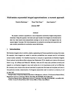
Figure 1: The contour plots of the log pseudo-posterior for different values of the temperature parameter. The prior is a product of two Student t(3) distributions. For a very large temperature, τ = 20, the first plot from the left, the posterior is very close to the prior. On the other extreme, for τ = .008, the utmost right plot, the posterior gets close to a Dirac mass at the observed data Y (here Y = [2, 1]). 2.1. Multivariate Regression Model We consider the model of multivariate regression with fixed design, in which we observe n featurelabel pairs (xi , Y i ), for i ∈ [n]. The labels Y i ∈ RK are random vectors with real entries, the features are assumed to be deterministic elements of an arbitrary space X . Note that, unless specified otherwise, we do not assume that the observations are independent. We introduce the regression function f ∗ : X → RK and noise vectors ξ i : F∗i = E[Y i ] = f ∗ (xi ),

ξ i = Y i − F∗i ,

i ∈ [n].

We are interested in estimating the values of f ∗ at the points x1 , . . . , xn only, which amounts to denoising the observed labels Y i . In such a setting, of course, one can forget about the features xi and the function f ∗ , since the goal is merely to estimate the K × n matrix F∗ = [F∗1 , . . . , F∗n ]. The b will be measured using the empirical loss quality of an estimator F b F∗ ) = `n (F,

1 b 1 X b kF − F∗ k2F = kFi − F∗i k22 . n n i∈[n]

This quantity is also referred to as in-sample prediction error. The following assumption will be repeatedly used. Assumption C(Bξ , L). For some positive numbers Bξ and L that, unless otherwise specified, may be equal to +∞, it holds that max P kξ i k22 > KBξ2 = 0, sup max kFi − F0i k22 ≤ KL2 . (1) i∈[n]

F,F0 ∈F i∈[n]

Note in (1) the presence of the normalizing factor K in the upper bounds on the Euclidean norms of K-dimensional vectors ξ i and (F − F0 )i . This allows us to think of the constants Bξ and L as dimension independent quantities.

3


2.2. Exponentially weighted aggregate The exponentially weighted aggregate (EWA) is defined as the average with respect to a tempered posterior distribution πn on F, the set of all K ×n matrices with real entries. To define the tempered posterior πn , we choose a prior distribution π0 on F and a temperature parameter τ > 0, and set n o πn (dF) ∝ exp − (1/2τ )`n (F, Y) π0 (dF). The EWA is then b EWA = F

Z F πn (dF).

(2)

F

According to the Varadhan-Donsker variational formula, the posterior distribution πn is the solution of the following optimisation problem: Z 1 πn ∈ arg min `n (F, Y) p(dF) + τ DKL (p k π0 ) , p F 2 where the inf is taken over all probability measures p on F. We see that the posterior distribution minimises a cost function which contains a term accounting for the fidelity to the observations and a regularisation term proportional to the divergence from the prior distribution. The larger the temperature τ , the closer the posterior πn is to the prior π0 . In most situations the integral in (2) cannot be computed in closed form. Even its approximate evaluation using a numerical scheme is often difficult. An appealing alternative is then to use Monte Carlo integration. This corresponds to drawing N samples F1 , . . . , FN from the posterior distribution πn and to define the Monte Carlo version of the EWA by N 1 X MC-EWA b F = F` . N `=1

Of course, the applicability of this method is limited to distributions πn for which the problem of sampling can be solved at low computational cost. We will see below that this approximation satisfies the same kind of oracle inequality as the original EWA.

3. PAC-Bayes type risk bounds In this section, we state and discuss several risk bounds for the EWA and related estimators under various conditions. We start with the case of the bounded regression vectors, i.e., the case where the constant L in Assumption C(Bξ , L) is finite. 3.1. Bounds without independence assumption but finite L We first state the results that hold even when the columns and rows of the noise matrix ξ are dependent. These results, however, require the boundedness of the set of aggregated elements F.

4


Theorem 1 Suppose that Assumption C(Bξ , L) is satisfied and the distribution of ξ is symmetric D

in the sense that for any sign vector s ∈ {±1}n , the equality in distribution [s1 ξ 1 , . . . , sn ξ n ] = ξ holds. Then, for every τ ≥ (1/n)(KBξ )(2L ∨ 3Bξ ), we have Z ∗ EWA ∗ b `n (F, F ) p(dF) + 2τ DKL (p ||π0 ) , (3) E[`n (F , F )] ≤ inf p

F

where the inf is taken over all probability measures on F. Furthermore, for larger values of the b =F b EWA temperature, τ ≥ (1/n)(KBξ )(2L ∨ 6Bξ ), the following upper bound holds for F Z Z 1 ∗ ∗ b b F)πn (dF)]. E[`n (F, `n (F, F ) p(dF) + 2τ DKL (p ||π0 ) − E[`n (F, F )] ≤ inf p 2 F F One can remark that the risk bound provided by (3) is an increasing function of the temperature. Therefore, the best risk bound is obtained for the smallest allowed value of temperature, that is τ=

K Bξ (2L ∨ 3Bξ ). n

Assuming Bξ and L as constants, while K = Kn can grow with n, we see that the remainder term in (3) is of the order K/n. We will see below that using other proof techniques, under somewhat different assumptions on the noise distribution, we can replace K by the spectral norm of the noise covariance matrix E[ξ i ξ > i ]. In the “worst case” when all the entries of ξ i are equal, these two 2 > 2 bounds are of the same order since kE[ξ i ξ > i ]k = E[ξi1 ]k1K 1K k = KE[ξi1 ]. Note, however, that the result above does not assume any independence condition on the noise vectors ξ i . Theorem 2 We assume that for some p × p matrix Σ 0, we have ξ = Σ1/2 ξ¯ where ξ¯ has independent rows ξ¯j• satisfying the following boundedness and symmetry conditions: ¯ξ ) = 1, • for any (i, j) ∈ [n] × [p], we have P(|ξ¯ji | ≤ B D • for any sign vector s ∈ {±1}n , the equality in distribution [s1 ξ¯j,1 , . . . , sn ξ¯j,n ] = ξ¯j• holds.

¯ > 0, we have maxi∈[n] kΣ1/2 (Fi − F0 )k∞ ≤ L ¯ for In addition, the set F is such that for some L i 0 ¯ξ )(2L ¯ ∨ 3kΣkB ¯ξ ), we have every F, F ∈ F. Then, for every τ ≥ (1/n)(B Z EWA ∗ ∗ b E[`n (F , F )] ≤ inf `n (F, F ) p(dF) + 2τ DKL (p ||π0 ) , p

F

where the inf is taken over all probability measures on F. Furthermore, for larger values of the b =F b EWA ¯ξ )(2L ¯ ∨ 6B ¯ξ ), the following upper bound holds for F temperature, τ ≥ (1/n)(B Z Z 1 b F∗ )] ≤ inf b F)πn (dF)]. E[`n (F, `n (F, F∗ ) p(dF) + 2τ DKL (p ||π0 ) − E[`n (F, p 2 F F The strength of this theorem is that it does not require the independence of the observations Y i corresponding to different values of i ∈ [n]. Only a symmetry condition is required. Furthermore, the resulting risk bound is valid for a temperature parameter which is of order O(1/n) and, hence, is independent of the dimension K of label vectors Y i . 5


The proofs of Theorem 1 and Theorem 2, postponed to Section 7, rely on the following interesting construction related to the Skorokhod embedding. If γ > 0 is a fixed number and ξ is a random variable having a symmetric distribution, then one can devise a new random variable ζ such that ξ + γζ has the same distribution as ξ and E[ζ | ξ] = 0. The construction of the pair (ξ, ζ) is as follows. We first draw a random variable R of the same distribution as |ξ| and a Brownian motion (Bt : t ≥ 0) independent of R. We then define the two stopping times T and Tγ by T = inf{t ≥ 0 : |Bt | = R},

Tγ = inf{t ≥ 0 : |Bt | = (1 + γ)R}.

One can easily check that the random variable BT has the same distribution as ξ whereas BTγ has the same distribution as (1 + γ)ξ. Furthermore, since conditionally to BT = x, the process (BT +t − x : t ≥ 0) is a Brownian motion, we have E[BTγ − BT |BT ] = 0. Therefore, the pair ξ := BT and ζ := (BTγ − BT )/γ satisfies the aforementioned conditions. If we set η = ζ/ξ, we can check that ( γ 1, with probability 1 − 1+2γ , η= γ 1 −1 − γ , with probability 1+2γ . This is exactly the formula used in Lemma 3 below. This particular example of the Skorokhod embedding relies heavily on the symmetry of the distribution of ξ. There are other constructions that do not need this condition. We believe that some of them can be used to further relax the assumptions of Theorem 1 and Theorem 2. This is, however, out of scope of the present work. 3.2. Bounds under independence with infinite L The previous two theorems require from the set F of aggregated elements to have a finite diameter ¯ and this diameter enters (linearly) in the risk bound through the temperature. The presence L (or L) of this condition is dictated by the techniques of the proofs; we see no reason for the established oracle inequalities to fail in the case of infinite L. In the present section, we state some results that are proved using another technique, building on the celebrated Stein lemma, which do not need L to be finite. Theorem 3 Assume that for some K × K positive semidefinite matrix Σ, the noise matrix ξ = Σ1/2 ξ¯ with ξ¯ satisfying the following conditions: C1. all the random variables ξ¯j,i are iid with zero mean and bounded variance, C2. the measure mξ¯(x) dx, where mξ¯(x) = −E[ξ¯j,i 1(ξ¯j,i ≤ x)], is absolutely continuous with respect to the distribution of ξ¯j,i with a Radon-Nikodym derivative2 gξ¯, C3. gξ¯ is bounded by some constant Gξ¯ < ∞. Then, for any τ ≥ (kΣkGξ¯)/n, we have b EWA , F∗ )] ≤ inf E[`n (F p

nZ

o `n (F, F∗ ) p(dF) + 2τ DKL (p k π0 ) .

F

b =F b EWA Furthermore, if τ ≥ 2(kΣkGξ¯)/n, then for F nZ o 1Z ∗ ∗ b b πn (dF) . E[`n (F, F )] = inf `n (F, F ) p(dF) + 2τ DKL (p k π0 ) − E `n (F, F) p 2 F F 2. This means that for any bounded and measurable function h, we have

6

R R

h(x)mξ¯(x) dx = E[h(ξ¯j,i )gξ¯(ξ¯j,i )].

(4)


As mentioned in (Dalalyan and Tsybakov, 2008, pp 43-44), many distributions satisfy assumptions C2 and C3. For instance, for the Gaussian distribution N (0, σ 2 ) and for the uniform in [−b, b] distributions these assumptions are fulfilled with Gξ¯ = σ 2 and Gξ¯ = b2 /2, respectively. More generally, if ξ¯j,i has a density pξ¯ with bounded support [−b, b], then the assumptions are satisfied with Gξ¯ = E[|ξ¯j,i |]/ min|x|≤b pξ¯(x). Here, we add another class to the family of distributions satisfying C2 and C3: unimodal distributions with compact support. Proposition 1 Assume that ξ¯j,i has a density pξ¯ with respect to the Lebesgue measure such that pξ¯(x) = 0 for every x 6∈ [−b, b] and, for some a ∈ [−b, b], pξ¯ is increasing on [−b, a] and decreasing on [a, b]. Then, ξ¯j,i satisfies C2 and C3 with Gξ¯ = (b2/2). Perhaps the most important shortcoming of the last theorem is that it cannot be applied to the discrete distributions of noise. In fact, if the distribution of ξ¯j,i is discrete, then there is no chance condition C2 to be satisfied. This is due to the fact that the measure mξ¯ dx, being absolutely continuous with respect to the Lebesgue measure, cannot be absolutely continuous with respect to a counting measure. On the other hand, Theorem 1 and Theorem 2 can be applied to discrete noise distributions, but they require boundedness of the family F. At this stage, we do not know whether it is possible to extend PAC-Bayesian type risk bound (4) to discrete distributions and unbounded sets F. However, in the case of a bounded discrete noise, we propose a simple modification of the EWA for which (4) is valid. The modification mentioned in the previous paragraph consists in adding a uniform noise to the entries of the observed labels Yi . Thus, we define the noisy exponential weighting aggregate, nEWA, by Z nEWA b ¯ π0 (dF), F = Fπ ¯n (dF), π ¯n (dF) ∝ exp − (1/2τ )`n (F, Y) (5) F

¯ = Y + ζ, with ζ a K × n where π ¯n is defined in the same way as πn but for the perturbed matrix Y random perturbation matrix. b nEWA be the noisy EWA defined by (5). Assume that Theorem 4 Let F C4. entries ξj,i of the noise matrix ξ are iid with zero mean and bounded by some constant Bξ > 0, C5. entries ζj,i of the perturbation matrix are iid uniformly distributed in [−Bξ , Bξ ]. Then, for any τ ≥ 2Bξ2 /n, we have b nEWA , F∗ )] ≤ inf E[`n (F p

nZ

o `n (F, F∗ ) p(dF) + 2τ DKL (p k π0 ) .

(6)

F

b =F b nEWA Furthermore, if τ ≥ 4Bξ2 /n, then for F b F∗ )] = inf E[`n (F, p

nZ

o 1Z b EWA ) π `n (F, F ) p(dF) + 2τ DKL (p k π0 ) − E `n (F, F ¯n (dF) . 2 F F ∗

¯ satisfies the conditions of Proof of Theorem 4. Let us check that the matrix of perturbed labels Y Theorem 3 with Σ = IK . To this end, we set ξej,i = ξj,i + ζj,i . We will check that the distribution 7


of ξej,i satisfies conditions C2 and C3 (condition C1 is straightforward). Since the distribution of ξej,i is the convolution of that of ξj,i and a uniform distribution, it admits a density with respect to the Lebesgue measure which is given by pe(x) =

1 1 P(|ξj,i − x| ≤ Bξ ) = P(ξj,i ∈ [x − Bξ , x + Bξ ] ∩ [−Bξ , Bξ ]). 2Bξ 2Bξ

The set Ax := [x − Bξ , x + Bξ ] ∩ [−Bξ , Bξ ] is empty if |x| > 2Bξ , increasing on the interval x ∈ [−2Bξ , 0] and decreasing on the interval x ∈ [0, 2Bξ ]. This implies that the density pe is zero outside the interval [−2Bξ , 2Bξ ] and unimodal in this interval. Therefore, it satisfies Proposition 1 with b = 2Bξ and a = 0. This implies that conditions C2 and C3 are fulfilled with Gξ¯ = 2Bξ2 and kΣk = 1. Thus, the conclusion of Theorem 3 applies and yields the claims of Theorem 4. ¯ where ξ¯j,i are iid and bounded. We can replace in Theorem 3 the condition C4 by ξ = Σ1/2 ξ, ¯ where ζ¯j,i ’s are iid uniform. In this case, the contamination added to the labels is of the form Σ1/2 ζ, The claims of Theorem 4 remain valid, but they are of limited interest, since it is not likely to find a situation in which the matrix Σ is known. 3.3. Risk bounds for the Monte Carlo EWA The four theorems of the previous sections contain all two risk bounds. The first bound is, in each case, more elegant and valid for a smaller value of the temperature than the second bound. However, the latter appears to be more useful for getting guarantees for the Monte Carlo version of the EWA. This is due to the fact that the additional term in the second risk bounds is proportional to the difference of the risks between the MC-EWA and the EWA. b MC-EWA is the MC-EWA with N Monte Carlo samples, then Proposition 5 If F Z 1 MC-EWA ∗ EWA ∗ b b b EWA ) πn (dF)]. E[`n (F , F )] = E[`n (F , F )] + E[`n (F, F N F Therefore, if the conditions of one of the four foregoing theorems are satisfied and τ is chosen accordingly then, as soon as N ≥ 2, nZ o b MC-EWA , F∗ )] ≤ inf `n (F, F∗ ) p(dF) + 2τ DKL (p k π0 ) . E[`n (F p

F

The proof of this result is straightforward and, therefore, is omitted. Note that this result bounds only the expected error, where the expectation is taken with respect to both the noise matrix ξ and the Monte Carlo sample. Using standard concentration inequalities, this bound can be complemented b MC-EWA and its “expectation” by an evaluation of the deviation between the Monte Carlo average F EWA b F . 3.4. Relation to previous work To the best of our knowledge, the first result in the spirit of the oracle inequalities presented in foregoing sections has been established by Leung and Barron (2006), using a technique heavily based on Stein’s unbiased risk estimate for regression with Gaussian noise developed in (George, 1986a,b). The first extensions to more general noise distributions were presented in (Dalalyan and Tsybakov, 8


2007, 2008) and later on refined in (Dalalyan and Tsybakov, 2012a). In all these papers, only the problem of aggregating “frozen” (that is independent of the data used for the aggregation) estimators. In his PhD thesis, Leung (2004) proved that analogous oracle bounds hold for the problem of aggregation of shrinkage estimators. The case of linear estimators has been explored by Dalalyan and Salmon (2012); Dai et al. (2014); Bellec (2018). In the context of sparsity, statistical properties of exponential weights were studied in Alquier and Lounici (2011); Rigollet and Tsybakov (2011, 2012). There is also extensive literature on the exponential weights for problems with iid obsrvations, such as the density model, the regression with random design, etc. We refer the interested reader to (Yang, 2000a,b; Catoni, 2007; Juditsky et al., 2008; Audibert, 2009; Dalalyan and Tsybakov, 2012b) and the references therein. It is useful to note here that the proof techniques used in the iid setting and in the setting with deterministic design considered in the present work are very different. Furthermore, the version exponential of the exponential weights used in the iid setting involves an additional averaging step and is therefore referred to as progressive mixture or mirror averaging.

4. EWA with low-rank favoring priors To give a concrete example of application of the results established in previous section, let us consider the so called reduced rank regression model. An asymptotic analysis of this model goes back to (Izenman, 1975), whereas more recent results can be found in (Bunea et al., 2011b, 2012) and the references therein. It corresponds to assuming that the matrix F∗ = E[Y] has a small rank, as compared to its maximal possible value K ∧ n. Equivalently, this means that the observed K dimensional vectors Y 1 , . . . ,Y n belong, up to a noise term, to a low dimensional subspace. Such problems arise, for instance, in subspace clustering or in multi-index problems. Of course, one can estimate the matrix F∗ by the PCA, but it requires rather precise knowledge of the rank. In order to get an estimator that takes advantage of the (nearly) low-rank property of the matrix F∗ , we suggest to use the following prior π0 (dF) ∝ det(λ2 IK + FF> )−(n+K+2)/2 dF,

(7)

where λ > 0 is a tuning parameter. From now on, with a slight abuse of notation, we will denote by π0 (F) the probability density function of the measure π0 (dF). The same will be done for p(dF) and πn (dF). We will refer to π0 as the spectral scaled Student prior, since one easily checks that π0 (F) ∝

K Y

(λ2 + sj (F)2 )−(n+K+2)/2 ,

j=1

where sj (F) denotes the jth largest singular value of F. We can recognize in the last display the density function of the scaled Student t evaluated at sj (F). Thus, the scaled spectral Student prior operates on the spectrum of F as the sparsity favoring prior introduced in (Dalalyan and Tsybakov, 2012a) on the vectors. Another interesting property of this prior, is that if F ∼ π0 , then the marginal distributions of the columns of F are scaled multivariate Studtent t3 . Lemma 1 If F is a random matrix having as density the function√π0 , then the random vectors Fi are all R drawn from the K-variate scaled Student distribution (λ/ 3)t3,K . As a consequence, we have F kFi k22 π0 (F) dF = λ2 K. 9


From a mathematical point of view, the nice feature of the aforementioned prior is that the ¯ version grows proportionally Kullback-Leibler divergence between π0 and its shifted by a matrix F ¯ to the rank of F, when all the other parameters remain fixed. This is formalized in the next result. Lemma 2 Let p¯ be the probability density function obtained from the prior π0 by a translation, ¯ Then, for any matrix F ¯ of at most rank r, we have p¯(F) = π0 (F − F). ¯ F kFk ¯ DKL (¯ p k π0 ) ≤ 2r(n + K + 2) log 1 + √ ≤ 2r(n + K + 2) log 1 + kFk/λ . 2rλ The proof of this result is deferred to the appendix. Applying this lemma, in conjunction with Theorem 3, we get a risk bound in the reduced rank regression problem which illustrates the power of the exponential weights. Theorem 6 Let the noise matrix ξ and the artificial perturbation matrix ζ satisfy the assumptions of Theorem 4. Let π0 be the scaled spectral Student prior (7) with some tuning parameter λ > 0. Then, for every τ ≥ 2Bξ2 /n, we have ¯ F kFk ∗ nEWA ∗ ¯ ¯ b E[`n (F , F )] ≤ inf `n (F, F ) + 4r(F)(n + K + 2)τ log 1 + √ + Kλ2 , ¯ F 2rλ

(8)

¯ where r(F) = rank(F) and the inf is taken over all K × n matrices F. ¯ and denote its rank by r. We apply Theorem 4 Proof of Theorem 6. Let us fix an arbitrary matrix F and upper bound the inf with respect to all probability distributions p by the right hand side of (6) evaluated at the distribution p¯ defined in Lemma 2. This yields Z ¯ F kFk nEWA ∗ ∗ b ¯ ¯ E[`n (F , F )] ≤ `n (F, F )π0 (F − F) dF + 4r(F)(n + K + 2)τ log 1 + √ . 2rλ F R Using the translation invariance of the Lebesgue measure and the fact that F π0 (F) dF = 0, we get Z Z ¯ dF = `n (F, ¯ F∗ ) + 1 `n (F, F∗ )π0 (F − F) kFk2F π0 (F) dF. n F F Let us focus on the evaluation of the last integral. ThePclaimed inequality follows from the last display by applying Lemma 1 and the fact that kFk2F = i∈[n] kFi k22 . There are many papers using Bayesian approach to the problem of prediction with low rank matrices, see (Alquier, 2013; Bouwmans et al., 2016) and the references therein. All the methods we are aware of define a prior on F using the following scheme: first choose a prior on the space of triplets (U, V, γ), where U and V are orthogonal matrices and γ is a vector with nonnegative entries, and then define π0 as the distribution of UD2γ V> (see, for instance, (Mai and Alquier, 2015b; Alquier and Guedj, 2017)). Similar type of priors have been also used in the problem of tensor decomposition and completion Rai et al. (2014) but, to date, their statistical accuracy has not been studied.

10


To our knowledge, (Yang et al., 2017) is the only work dealing with prior (7) in a context related to low rank matrix estimation and completion. It proposes variational approximations to the Bayes estimator and demonstrates their good performance on various data sets. In a sense, Theorem 6 provides theoretical justification for the empirically observed good statistical properties of the prior defined in (7). Let us briefly discuss the inequality of Theorem 6. Assume that we choose τ = 2Bξ2 /n and λ2 = Bξ2 (n + K)/K. Then, we see that (8) handles optimally mis-specification, since it is an oracle inequality with a leading constant 1, and the remainder term is of optimal order r(n + K)/n, up to a logarithmic factor. Other oracle inequalities with nearly optimal remainder terms in the context of low-rank matrix estimation and completion are exposed in (Mai and Alquier, 2015a; Alquier, 2013; Alquier and Guedj, 2017). However, those results are not sharp oracle inequalities since the factor in front of the leading term in the upper bound is larger than 1. Using the properties of the scaled Student prior exposed in Lemma 1 and Lemma 2, one can establish oracle inequalities in other statistical problems in which the unknown parameter is a matrix, such as matrix completion, trace regression or multiclass classification, see (Srebro and Shraibman, 2005; Rohde and Tsybakov, 2011; Koltchinskii et al., 2011; Candès and Tao, 2010; Candès and Plan, 2011; Bunea et al., 2011a; Ga¨ıffas and Lecué, 2011; Negahban and Wainwright, 2011, 2012; Klopp, 2014; Dalalyan et al., 2016). This is left to future work.

5. Implementation and a few numerical experiments In this section, we report the results of some proof of concept numerical experiments. We propose to compute an approximation of the EWA with the scaled multivariate Student prior by a suitable version of the Langevin Monte Carlo algorithm. To describe the letter, let us first remark that log πn (F) = −

1 (n + K + 2) `n (F, Y) − log det(λ2 IK + FF> ). 2τ 2

(9)

From this relation, we can infer that −∇ log πn (F) =

1 (F − Y) + (n + K + 2)(λ2 IK + FF> )−1 F. nτ

The (constant-step) Langevin MC is defined by choosing an initial matrix F0 and then by using the recursion √ Fk+1 = Fk + h∇ log πn (F) + 2h Wk , k = 0, 1, . . . , where h > 0 is the step-size and W0 , W1 , . . . are independent Gaussian random matrices with iid standard Gaussian entries. For (strongly) log-concave densities π, nonasymptotic guarantees for the LMC have been recently established in Dalalyan (2017); Durmus and Moulines (2016), but they do not carry over the present case since the right hand side of (9) is not concave. Our numerical experiments show that (despite the absence of theoretical guarantees) the LMC converges and leads to relevant results. Note that a direct application of the Langevin MC algorithm involves a K × K matrix inversion at each iteration. This might be costly and can slow down significantly the algorithm. We suggest to replace this matrix inversion by a few steps of gradient descent for a suitably chosen optimization

11


problem. Indeed, one can easily check that the matrix M = (λ2 IK + FF> )−1 F is nothing else but the solution to the convex optimization problem min kIn − F> Mk2F + 2λ2 kMk2F . We use ten gradient descent steps for approximating the solution of this optimization problem. This does not require neither matrix inversion nor svd or other costly operation. Theoretical assessment of the Langevin MC with inaccurate gradient evaluations can be found in Dalalyan and Karagulyan (2017). We applied this algorithm to the problem of image denoising. We chose an RGB image of resolution 120 × 160 and applied to it an additive Gaussian white noise of standard deviation σ ∈ {10, 30, 50}. In order to make use of the denoising algorithm based on the aforementioned Langevin MC, we transformed the noisy image into a matrix of size 192 × 300. Each row of this transformed matrix corresponds to a patch of size 10 × 10 × 3 of the noisy image. The patches are chosen to be non-overlapping in order to get a reasonable dimensionality. We expect the result to be better for overlapping patches, but the computational cost will also be high. The parameters were chosen as follows: p τ = 2σ 2 /n; λ = 10σ (n + K)/K; h = 10; kmax = 4000. Note that the values of τ and λ are suggested by our theoretical results, while the step-size h and the number of iterations of the LMC, kmax , were chosen experimentally. The LMC after kmax iterations provides one sample that is approximately drawn from the pseudo-posterior πn . We did N = 400 repetitions and averaged the obtained results for approximating the posterior mean.

6. Conclusion We have studied the expected in-sample prediction error of the Exponentially Weighted Algorithm (EWA) in the context of multivariate regression with possible dependent noise. We have shown that under boundedness assumptions on the noise and the aggregated elements, the EWA satisfies a PAC-Bayes type sharp oracle inequality, provided that the temperature parameter is sufficiently large. The remainder term in these oracle inequalities is of arguably optimal order of magnitude and is consistent with the corresponding results obtained in the model of univariate regression. An interesting observation is that if we apply the EWA to the data matrix artificially contaminated by a uniform noise, the resulting procedure satisfies a sharp oracle inequality under a much weaker assumption on the noise distribution. In particular, this allows to cover any distribution with bounded support. We have also included the results of a small numerical experiment on image denoising, that shows the applicability of the EWA.

7. Proofs of the main results The proofs of all the main theorems stated in the previous sections are gathered in this section. The proofs of some technical lemmas are deferred to Appendix A. b EWA , F∗ ). Let ζ be a random matrix such that Proof of Theorem 1. We wish to upper bound `n (F E[ζ|Y] = 0 and define `n (F, F∗ , ζ) = `n (F, F∗ ) +

12

2 hζ, F − F∗ i. n


True image Original Image

Original Image

Noisy image Noisy Image

Restaured image Restaured Image

σ = 50, PSNR = 14.1

PSNR = 20.6

Noisy Image

σ = 30, PSNR = 18.6

Restaured Image

PSNR = 24.3

Original Image

Noisy Image

Original Image

σ = 20,Noisy PSNR = 22.1 Image

PSNR = 27.1 Restaured Image

σ = 10, PSNR = 28.1

PSNR = 32.2

Original Image

Noisy Image

σ = 5, PSNR = 34.1

Restaured Image

Restaured Image

PSNR = 36.7

Figure 2: The result of the experiment on image densoising. Left: the original 120×160×3 image. Middle: the noisy image for different values of σ. Right: the denoised image.

13


b instead of F b EWA . We have, for every α > 0, In what follows, we use the short notation F n o 1 ∗ ∗ b b `n (F, F , ζ) = log exp α `n (F, F , ζ) α Z Z 1 1 ∗ b ∗ ,ζ)−`n (F,F∗ ,ζ) α `n (F,F πn (dF) − log e e−α `n (F,F ,ζ) πn (dF) . = log α α F F | | {z } {z } :=S1 (α)

:=S(α)

The next two lemmas provide suitable upper bounds on the magnitude of the terms S(α) and S1 (α). Lemma 3 Let ξ = [ξ 1 , . . . , ξ n ] be a K × n random matrix with real entries having a symmetric distribution (see the statement of Theorem 1). Let ζ i be defined as ζ i = ξ i ηi , where ηi are iid random variables independent of ξ and satisfying ( ατ 1, with probability 1 − 1+2ατ , ηi = ατ 1 −1 − ατ , with probability 1+2ατ . Then, the expectation of the random variable S can be bounded as follows: Z ∗ `n (F, F ) p(dF) + 2τ DKL (p ||π0 ) , −(1/α) E[S(α)] ≤ inf p

F

where the inf is taken over all probability measures on F. Lemma 4 Let the random vectors ζ i , i ∈ [n] be as defined in Lemma 3. Then, we have Z Z X 1 b i −Fi ) −(2/nτ )ξ> (F b F)πn (dF). i lim E[S1 (α) | ξ] ≤ τ log e πn (dF) − `n (F, α→0 α F F i∈[n]

Applying these two lemmas, we get b F∗ )] = E[`n (F, b F∗ , ζ)] = lim E(E[S1 (α)|ξ]) − E[S(α)] E[`n (F, α→0 α Z Z ∗ b F)πn (dF) ≤ inf `n (F, F ) p(dF) + 2τ DKL (p ||π0 ) − `n (F, p F F Z X b i −Fi ) −(2/nτ )ξ> (F i + τ E log e πn (dF) . (10) F

i∈[n]

Then, for every τ ≥ (2K/n)(Bξ L), we have >

e−(2/nτ )ξi

This implies that Z

b i −Fi ) (F

b −(2/nτ )ξ> i (Fi −Fi )

e

2 b b 3(ξ > 2ξ > i (Fi − Fi ) i (Fi − Fi )) + nτ (nτ )2 b i − Fi k 2 b i − Fi ) 3KBξ2 kF 2ξ > (F 2 ≤1− i + . nτ (nτ )2

≤1−

πn (dF) ≤ 1 +

F

14

3KBξ2 (nτ )2

Z F

b i − Fi k2 πn (dF). kF 2


Combining the last display with (10) and using the inequality log(1 + x) ≤ x, we arrive at Z ∗ ∗ b `n (F, F ) p(dF) + 2τ DKL (p ||π0 ) E[`n (F, F )] ≤ inf p

F

− 1−

3KBξ2 nτ

Z E

b F)πn (dF) . `n (F,

F

This completes the proof of the theorem. Proof of Theorem 2. The proof follows the same arguments as those used in the proof of Theorem 1. That is why, we will skip some technical details. The main difference is in the definition of the matrix ζ and the subsequent computations related to the evaluation of the term S2 (α). Thus, for any random matrix ζ such that E[ζ|Y] = 0 and for `n (F, F∗ , ζ) = `n (F, F∗ ) + n2 hζ, F − F∗ i, we have b F∗ )] = E[`n (F, b F∗ , ζ)] = lim E[S1 (α)] − E[S(α)] , E[`n (F, α→0 α where S and S1 are the same as in the proof of Theorem 1. We instantiate the matrix ζ as follows: ζ = Σ1/2 ζ¯ where the entries of ζ¯ are given by ζ¯j,i = ξ¯j,i ηj,i , with ηj,i being iid random variables independent of ξ and satisfying ( ατ , 1, with probability 1 − 1+2ατ ηj,i = ατ 1 −1 − ατ , with probability 1+2ατ . One easily checks that the resulting vector ξ¯j• +2ατ ζ¯ j,• has the same distribution as the vector (1+ 2ατ )ξ¯j,• , for every j ∈ [K]. Furthermore, for different values of j, these vectors are independent. ¯ which is This implies that the matrix ξ¯ + 2ατ ζ¯ has the same distribution as the matrix (1 + 2ατ )ξ, sufficient for getting the conclusion of Lemma 3. That is Z −(1/α) E[S(α)] ≤ inf `n (F, F∗ ) p(dF) + 2τ DKL (p ||π0 ) , p

F

where the inf is taken over all probability measures on F. To bound the term S1 , we use a result similar to that of Lemma 4. b − F). Then, we Lemma 5 Let the random matrix ζ be defined as above. Set H(F) = Σ1/2 (F have Z Z X 1 ¯ b F)πn (dF). lim E[S1 (α) | ξ] ≤ τ log e−(2/nτ )ξj,i Hj,i (F) πn (dF) − `n (F, α→0 α F F i∈[n] j∈[K]

¯ξ L), ¯ we have Then, for every τ ≥ (2/n)(B e

−(2/nτ )ξ¯j,i Hj,i (F)

2 H (F)2 2ξ¯j,i Hj,i (F) 3ξ¯j,i j,i ≤1− + nτ (nτ )2 ¯ 2 H2 (F) 2ξ¯j,i Hj,i (F) 3B ξ j,i ≤1− + . nτ (nτ )2

15


R

Using the fact that

F

Z

H(F) πn (dF) = 0, the last display implies that ¯2 3B ξ

¯

e−(2/nτ )ξj,i Hj,i (F) πn (dF) ≤ 1 +

F

(nτ )2

Z F

H2j,i (F)πn (dF).

Combining the last display with Lemma 5 and using the inequality log(1 + x) ≤ x, we arrive at Z ¯2 Z X 3B 1 ξ 2 b F)πn (dF) `n (F, lim E[S1 (α) | ξ] ≤ H (F)πn (dF) − α→0 α n2 τ F j,i F i,j Z ¯2 Z 3B ξ b F)πn (dF) b − F)k2 πn (dF) − = 2 `n (F, kΣ1/2 (F F n τ F F ¯2 Z 3Bξ kΣk b F)πn (dF). ≤ −1 `n (F, nτ F This completes the proof of the theorem. Proof of Theorem 3. We outline here only the main steps of the proof, without going too much into the details. One can extend the Stein lemma from the Gaussian distribution to that of ξ¯j,i , provided the conditions of Theorem 3 are satisfied (see Lemma 1 in (Dalalyan and Tsybakov, 2008) for a similar result). The resulting claim is that the random variable n

K

XX b Y) − tr(Σ) + 2 b j,i rb := `n (F, gξ¯(ξ¯j,i )∂ξ¯j,i (Σ1/2 F) n

(11)

i=1 j=1

b F∗ )]. On the one hand, using Varadhan-Donsker’s variational formula, we satisfies E[b r] = E[`n (F, get b Y)] ≤ E[`n (F, b Y) + 2τ DKL (πn k π0 )] E[`n (F, hZ i Z b πn (dF) =E `n (F, Y) πn (dF) + 2τ DKL (πn k π0 ) − E `n (F, F) F Z F h i Z b πn (dF) ≤ E inf `n (F, Y) p(dF) + 2τ DKL (p k π0 ) − E `n (F, F) p F F h Z i Z b πn (dF) ≤ inf E `n (F, Y) p(dF) + 2τ DKL (p k π0 ) − E `n (F, F) p F F Z b πn (dF) . = inf `n (F, F∗ ) + tr(Σ) + 2τ DKL (p k π0 ) − E `n (F, F) p

F

b j,i , we get On the other hand, computing the partial derivative ∂Yj,i (Σ1/2 F) b j,i = e> Σ1/2 (∂¯ F b ∂ξ¯j,i (Σ1/2 F) j ξi i )ej Z 1 > 1/2 b i (F b i − Yi )> Σ1/2 ej ej Σ Fi (Fi − Yi )> πn (dF) − F = 2nτ F Z > 1/2 1 b i 2 πn (dF). = ej Σ (F − F) 2nτ F 16


From this relation, we infer that K X

Z K > 1/2 1 X b i 2 πn (dF) gξ¯(ξ¯j,i ) ej Σ (F − F) 2nτ F j=1 Z Gξ¯ b i )k2 πn (dF) ≤ kΣ1/2 (Fi − F 2 2nτ F Z kΣkGξ¯ b i k2 πn (dF). ≤ kFi − F 2 2nτ F

b j,i = gξ¯(ξ¯j,i )∂Yj,i (Σ1/2 F)

j=1

(12)

Combining (11)-(12), we arrive at b F∗ )] = E[b E[`n (F, r] Z b πn (dF) E `n (F, F) ≤ inf `n (F, F∗ ) + 2τ DKL (p k π0 ) − p

F

n Z kΣkGξ¯ X b i − Fi k2 πn (dF)] + E[kF 2 n2 τ i=1 F Z kΣkGξ¯ ∗ b πn (dF) . = inf `n (F, F ) + 2τ DKL (p k π0 ) − 1 − E `n (F, F) p nτ F

This completes the proof. Proof of Proposition 1. Without loss of generality, we assume that a ≥ 0. We have, for every x ∈ [a, b], Z mξ¯(x) =

b

x

Z ypξ¯(y) dy ≤ pξ¯(x)

b

x

y dy ≤ (b2/2)pξ¯(x).

Similarly, for every x ∈ [−b, 0], we have x ≤ a and, therefore, Z x Z x mξ¯(x) = − ypξ¯(y) dy ≤ pξ¯(x) (−y) dy ≤ (b2/2)pξ¯(x). −b

−b

Finally, for x ∈ [0, a], we have Z mξ¯(x) =

x

−b

Z (−y)pξ¯(y) dy ≤

0

−b

(−y)pξ¯(y) dy ≤ (b2/2)pξ¯(0) ≤ (b2/2)pξ¯(x)

and the claim of the lemma follows.

Acknowledgments This work was partially supported by the grant Investissements d’Avenir (ANR-11-IDEX-0003/Labex Ecodec/ANR-11-LABX-0047) and the chair “LCL/GENES/Fondation du risque, Nouveaux enjeux pour nouvelles donnes”.

17


References P. Alquier and B. Guedj. An oracle inequality for quasi-bayesian nonnegative matrix factorization. Mathematical Methods of Statistics, 26(1):55–67, Jan 2017. ISSN 1934-8045. doi: 10.3103/ S1066530717010045. URL https://doi.org/10.3103/S1066530717010045. Pierre Alquier. Bayesian methods for low-rank matrix estimation: Short survey and theoretical study. In Sanjay Jain, Rémi Munos, Frank Stephan, and Thomas Zeugmann, editors, Algorithmic Learning Theory, pages 309–323, Berlin, Heidelberg, 2013. Springer Berlin Heidelberg. Pierre Alquier and Karim Lounici. PAC-Bayesian bounds for sparse regression estimation with exponential weights. Electron. J. Stat., 5:127–145, 2011. Jean-Yves Audibert. Fast learning rates in statistical inference through aggregation. Ann. Statist., 37(4):1591–1646, 2009. Pierre C. Bellec. Optimal bounds for aggregation of affine estimators. Ann. Statist., 46(1):30–59, 02 2018. doi: 10.1214/17-AOS1540. Thierry Bouwmans, Necdet Serhat Aybat, and El-Hadi Zahzah. Handbook on ”Robust Low-Rank and Sparse Matrix Decomposition: Applications in Image and Video Processing”. CRC Press, Taylor and Francis Group, , May 2016. URL https://hal.archives-ouvertes.fr/ hal-01373013. Florentina Bunea, Yiyuan She, and Marten H. Wegkamp. Optimal selection of reduced rank estimators of high-dimensional matrices. Ann. Statist., 39(2):1282–1309, 2011a. Florentina Bunea, Yiyuan She, and Marten H. Wegkamp. Optimal selection of reduced rank estimators of high-dimensional matrices. Ann. Statist., 39(2):1282–1309, 04 2011b. doi: 10.1214/11-AOS876. URL https://doi.org/10.1214/11-AOS876. Florentina Bunea, Yiyuan She, and Marten H. Wegkamp. Joint variable and rank selection for parsimonious estimation of high-dimensional matrices. Ann. Statist., 40(5):2359–2388, 10 2012. doi: 10.1214/12-AOS1039. URL https://doi.org/10.1214/12-AOS1039. Emmanuel J. Candès and Yaniv Plan. Tight oracle inequalities for low-rank matrix recovery from a minimal number of noisy random measurements. IEEE Trans. Inform. Theory, 57(4):2342–2359, 2011. Emmanuel J. Candès and Terence Tao. The power of convex relaxation: near-optimal matrix completion. IEEE Trans. Inform. Theory, 56(5):2053–2080, 2010. Olivier Catoni. Pac-Bayesian supervised classification: the thermodynamics of statistical learning. Lecture Notes–Monograph Series, 56. Institute of Mathematical Statistics, Beachwood, OH, 2007. Dong Dai, Philippe Rigollet, Lucy Xia, and Tong Zhang. Aggregation of affine estimators. Electron. J. Stat., 8(1):302–327, 2014. A. S. Dalalyan and A. B. Tsybakov. Sparse regression learning by aggregation and Langevin MonteCarlo. J. Comput. System Sci., 78(5):1423–1443, 2012a. 18


Arnak S. Dalalyan. Theoretical guarantees for approximate sampling from a smooth and logconcave density. to appear in JRSS B , arXiv:1412.7392, December 2017. Arnak S. Dalalyan and Avetik Karagulyan. User-friendly guarantees for the langevin monte carlo with inaccurate gradient. submitted 1710.00095, arXiv, October 2017. URL https://arxiv. org/abs/1710.00095. Arnak S. Dalalyan and Joseph Salmon. Sharp oracle inequalities for aggregation of affine estimators. Ann. Statist., 40(4):2327–2355, 2012. Arnak S. Dalalyan and Alexandre B. Tsybakov. Aggregation by exponential weighting and sharp oracle inequalities. In Learning theory, volume 4539 of Lecture Notes in Comput. Sci., pages 97–111. Springer, Berlin, 2007. Arnak S. Dalalyan and Alexandre B. Tsybakov. Aggregation by exponential weighting, sharp pacbayesian bounds and sparsity. Machine Learning, 72(1-2):39–61, 2008. Arnak S. Dalalyan and Alexandre B. Tsybakov. Mirror averaging with sparsity priors. Bernoulli, 18(3):914–944, 2012b. Arnak S. Dalalyan, Edwin Grappin, and Quentin Paris. On the exponentially weighted aggregate with the laplace prior. to appear in the Annals of Statistics 1611.08483, arXiv, November 2016. URL https://arxiv.org/abs/1611.08483. A. Durmus and E. Moulines. Sampling from strongly log-concave distributions with the Unadjusted Langevin Algorithm. Technical Report , arXiv:1605.01559, May 2016. Stéphane Ga¨ıffas and Guillaume Lecué. Sharp oracle inequalities for high-dimensional matrix prediction. IEEE Trans. Inform. Theory, 57(10):6942–6957, 2011. E. I. George. Minimax multiple shrinkage estimation. Ann. Statist., 14(1):188–205, 1986a. E. I. George. Combining minimax shrinkage estimators. J. Amer. Statist. Assoc., 81(394):437–445, 1986b. Alan Julian Izenman. Reduced-rank regression for the multivariate linear model. Journal of Multivariate Analysis, 5(2):248 – 264, 1975. ISSN 0047-259X. doi: https://doi.org/ 10.1016/0047-259X(75)90042-1. URL http://www.sciencedirect.com/science/ article/pii/0047259X75900421. A. Juditsky, P. Rigollet, and A. B. Tsybakov. Learning by mirror averaging. Ann. Statist., 36(5): 2183–2206, 2008. Olga Klopp. Noisy low-rank matrix completion with general sampling distribution. Bernoulli, 20 (1):282–303, 2014. Vladimir Koltchinskii, Karim Lounici, and Alexandre B. Tsybakov. Nuclear-norm penalization and optimal rates for noisy low-rank matrix completion. The Annals of Statistics, 39(5):2302–2329, 2011.

19


G. Leung. Information Theory and Mixing Least Squares Regression. PhD thesis, Yale University, 2004. Gilbert Leung and Andrew R. Barron. Information theory and mixing least-squares regressions. IEEE Trans. Inform. Theory, 52(8):3396–3410, 2006. The Tien Mai and Pierre Alquier. A Bayesian approach for noisy matrix completion: optimal rate under general sampling distribution. Electron. J. Stat., 9(1):823–841, 2015a. The Tien Mai and Pierre Alquier. A bayesian approach for noisy matrix completion: Optimal rate under general sampling distribution. Electron. J. Statist., 9(1):823–841, 2015b. doi: 10.1214/ 15-EJS1020. URL https://doi.org/10.1214/15-EJS1020. Sahand Negahban and Martin J. Wainwright. Estimation of (near) low-rank matrices with noise and high-dimensional scaling. Ann. Statist., 39(2):1069–1097, 2011. Sahand Negahban and Martin J. Wainwright. Restricted strong convexity and weighted matrix completion: optimal bounds with noise. J. Mach. Learn. Res., 13:1665–1697, 2012. Piyush Rai, Yingjian Wang, Shengbo Guo, Gary Chen, David Dunson, and Lawrence Carin. Scalable bayesian low-rank decomposition of incomplete multiway tensors. In Eric P. Xing and Tony Jebara, editors, Proceedings of the 31st International Conference on Machine Learning, volume 32 of Proceedings of Machine Learning Research, pages 1800–1808, Bejing, China, 22–24 Jun 2014. PMLR. Philippe Rigollet and Alexandre Tsybakov. Exponential screening and optimal rates of sparse estimation. Ann. Statist., 39(2):731–771, 2011. Philippe Rigollet and Alexandre B. Tsybakov. Sparse estimation by exponential weighting. Statist. Sci., 27(4):558–575, 2012. Angelika Rohde and Alexandre B. Tsybakov. Estimation of high-dimensional low-rank matrices. Ann. Statist., 39(2):887–930, 2011. Nathan Srebro and Adi Shraibman. Rank, trace-norm and max-norm. In Peter Auer and Ron Meir, editors, 18th Annual Conference on Learning Theory, COLT 2005. Proceedings, pages 545–560, 2005. Linxiao Yang, Jun Fang, Huiping Duan, Hongbin Li, and Bing Zeng. Fast low-rank bayesian matrix completion with hierarchical gaussian prior models. CoRR, abs/1708.02455, 2017. URL http://arxiv.org/abs/1708.02455. Y. Yang. Combining different procedures for adaptive regression. J. Multivariate Anal., 74(1): 135–161, 2000a. Y. Yang. Adaptive estimation in pattern recognition by combining different procedures. Statist. Sinica, 10(4):1069–1089, 2000b.

20


Appendix A. Proofs of technical lemmas Proof of Lemma 3. Using the fact that πn (dF) ∝ exp − (1/2τ )`n (F, Y) π0 (dF) and that `n (F, Y) = `n (F, F∗ ) + (2/n)hξ, F∗ − Fi + (1/n)kξk2F , we arrive at Z ∗ ∗ 1 1 −S(α) = log e−( /2τ )`n (F,F )−( /nτ )hξ,F −Fi π0 (dF) F Z ∗ ∗ 1 1 − log e−(α+ /2τ )`n (F,F )−( /nτ )hξ+2ατ ζ,F −Fi π0 (dF) F

One easily checks that the random matrix ξ + 2ατ ζ has the same distribution as the matrix (1 + 2ατ )ξ and, therefore, Z h i ∗ ∗ 1 1 −E[S(α)] = E log e−( /2τ )`n (F,F )−( /nτ )hξ,F −Fi π0 (dF) F Z h i −(2ατ +1) 1/2τ `n (F,F∗ )+(1/nτ )hξ,F∗ −Fi − E log e π0 (dF) . F

Applying the Hölder inequality the right hand side, we get

R

G dπ0 ≤

F

h 2ατ −E[S(α)] ≤ − E log 2ατ + 1

Z

R F

G2ατ +1 dπ0

e−(2ατ +1)

1/(2ατ +1)

to the first expectation of

1/2τ `n (F,F∗ )+(1/nτ )hξ,F∗ −Fi

i π0 (dF) .

F

Donsker-Varadhan’s variational inequality implies that h nZ oi 1 2τ − E[S(α)] ≤ E inf `n (F, F∗ ) + (2/n)hξ, F∗ − Fi p(dF) + DKL (p ||π0 ) p α 2ατ + 1 F nZ o 2τ ≤ inf E `n (F, F∗ ) + (2/n)hξ, F∗ − Fi p(dF) + DKL (p ||π0 ) p 2ατ + 1 F nZ o 2τ ≤ inf E `n (F, F∗ ) p(dF) + DKL (p ||π0 ) . p 2ατ + 1 F The desired result follows from the last display using the inequality 2ατ + 1 ≥ 1. Proof of Lemma 4. We have b F∗ , ζ) − `n (F, F∗ , ζ) = `n (F, b F∗ ) − `n (F, F∗ ) + 2 hζ, F b − Fi `n (F, n which implies that, Z S1 (α) = log

e

b ∗ )−`n (F,F∗ )+ 2 hζ,F−Fi b α `n (F,F n

πn (dF).

F

Using the definition of the expectation, we get Ψ(α) := E[S1 (α) | ξ ] Z X (ατ )ksk1 (1 + ατ )n−ksk1 = log eΦ(α,s,F) πn (dF), n (1 + 2ατ ) F n s∈{0,1}

21


where n n X 1 o b F∗ ) − `n (F, F∗ ) + 2 b i − Fi i. Φ(α, s, F) := α `n (F, α(1 − si ) − si α + hξ i , F n τ i=1

One easily checks that the function Ψ(α) is differentiable in (0, ∞) and that Ψ(0) = 0. Therefore, Ψ(α) Ψ(α) − Ψ(0) = lim = Ψ0 (0) α→0 α α→0 α Z X (ατ )ksk1 (1 + ατ )n−ksk1 d eΦ(α,s,F) πn (dF). log = dα (1 + 2ατ )n lim

(13)

F

α=0 s∈{0,1}n ksk1 ≤1

Let us now compute the derivatives with respect to α of the terms of the last sum. For the term corresponding to s = 0, since Φ(0, 0, F) = 0, we have Z Z d (1 + ατ )n d Φ(α,0,F) Φ(α,0,F) log e πn (dF) = log e πn (dF) dα α=0 (1 + 2ατ )n dα α=0 F Z F d Φ(α,0,F) e πn (dF) = dα α=0 F Z d Φ(α, 0, F) πn (dF). = F dα α=0 R b we arrive Using that Φ(α, 0, F) is a linear function of α, as well as the fact that F πn (dF) = F, at Z Z d (1 + ατ )n Φ(α,0,F) b F) πn (dF). log e π (dF) = − `n (F, n dα α=0 (1 + 2ατ )n F F Let us go back to (13) and evaluate the terms corresponding to vectors s such that ksk1 = 1. This means that only one entry of s is equal to one, all the others being equal to zero. Hence, if we denote by ei the ith element of the canonical basis of Rn , we get Z X (ατ )ksk1 (1 + ατ )n−ksk1 d log eΦ(α,s,F) πn (dF) n dα α=0 (1 + 2ατ ) F n s∈{0,1} ksk1 =1

Z n−1 X d (ατ )(1 + ατ ) = log eΦ(α,ei ,F) πn (dF) dα α=0 (1 + 2ατ )n F i∈[n] Z Z X X > b Φ(0,ei ,F) = τ log e πn (dF) = τ log e−(2/nτ )ξi (Fi −Fi ) πn (dF). i∈[n]

F

i∈[n]

F

This completes the proof of the lemma. Proof of Lemma 1. For any bounded and measurable function h : RK → R, we have Z Z h(F1 ) (a) 1 h(F1 ) π0 (F) dF = dF 2 Cλ F det(λ IK + FF> )(n+K+2)/2 F Z h(λM1 ) (b) 1 = dM C1 F det(IK + MM> )(n+K+2)/2 22


R where in (a) we have used the notation Cλ = F det(λ2 IK + FF> )−(n+K+2)/2 dF, whereas in (b) we have made the change of variable F = λM. In order to compute the last integral, we make ¯ given by M = [M ¯ 1 , (I + M ¯ 1M ¯ > )1/2 M ¯ 2:n ]. This yields another change of variable, M M, 1 ¯ 1 det(I + M ¯ 1M ¯ > )(n−1)/2 dM ¯ 2:n dM = dM1 dM2:n = dM 1 (c)

¯ 1 k2 )(n−1)/2 dM ¯ 1 dM ¯ 2:n = (1 + kM 2

and > det(I + MM> ) = det I + M1 M> 1 + M2:n M2:n ¯ 1M ¯ > + (I + M ¯ 1M ¯ > )1/2 M ¯ 2:n M ¯ > (I + M ¯ 1M ¯ > )1/2 = det I + M 1 1 2:n 1 ¯ 1M ¯ > )1/2 (I + M ¯ 2:n M ¯ > )(I + M ¯ 1M ¯ > )1/2 = det (I + M 1

2:n

1

¯ 1M ¯ > )det(I + M ¯ 2:n M ¯> ) = det(I + M 1 2:n (c0 )

¯ 1 k2 )det(I + M ¯ 2:n M ¯ > ), = (1 + kM 2 2:n

¯ 1M ¯ > has all its eigenvalues equal where in (c) and (c0 ) we have used the fact that the matrix I + M 1 ¯ 1 , which is equal to 1 + kM ¯ 1 k2 . to 1 except the largest one, corresponding to the eigenvector M 2 ¯ Using the same change of variable in C1 , and replacing M1 by x for convenience, we get R Z 2 −(K+3)/2 dx K h(λx)(1 + kxk2 ) h(F1 ) π0 (F) dF = R R 2 −(K+3)/2 dx F RK (1 + kxk2 ) √ R 3)(1 + kyk22 /3)−(K+3)/2 dy RK h(λy/ R . = 3 RK (1 + kyk22 /3)−(K+3)/2 dy In the last expression, we recognize the probability density function of the multivariate t3 -distribution. ν Since the covariance matrix of a K-variate tν distribution is equal to ν−2 IK , we infer that Z kFk2F π0 (F) dF = nKλ2 . F

This completes the proof of the lemma. Proof of Lemma 2. It holds that Z

π (F) 0 π0 (F) dF p¯(F) ZF π (F) 0 = log ¯ π0 (F) dF. π (F − F) 0 F

DKL (¯ pkπ0 ) =

log

¯ ¯ > . We have To ease notation, we set A = (λ2 IK + FF> )−1/2 and B = λ2 IK + (F − F)(F − F) π (F) det(B) 0 2 log = (n + K + 2) log (14) ¯ det(A−2 ) π0 (F − F) = (n + K + 2) log det(ABA) = (n + K + 2)

K X j=1

23

log sj (ABA),


where sj (ABA) is the jth largest eigenvalue of the symmetric matrix ABA. Let r be the rank ¯ The first claim is that the matrix ABA has at most 2r singular values different from one. of F. Indeed, one can check that ¯ ∗> A − AFF ¯ > A − AFF ¯ > A. ABA − IK = AFF The matrix at the right hand side is at most of rank 2r. This implies that ABA − IK has at most 2r nonzero eigenvalues. Therefore, the number of eigenvalues of ABA different from 1 is not larger than 2r, which implies that the sum at the right hand side of (14) has at most 2r nonzero entries. Let uj be the unit eigenvector corresponding to the eigenvalue sj . We know that, for every j ∈ [2r], sj = u> j ABAuj . Using , we get ¯ ∗> ¯ > ¯> sj = 1 + u> j (AFF A − AFF A − AFF A)uj ¯ > Auj k2 + k(F ¯ − F)> Auj k2 = 1 − kF 2

¯>

2

2

≤ (1 + kF Auj k2 ) . Using the concavity of the function log(1 + x1/2 ) over (0, +∞), we arrive at 2 log

2r X π0 (F) = (n + K + 2) log sj (ABA) ¯ π0 (F − F) j=1

≤ 2(n + K + 2)

2r X

> ¯ Auj k2 1/2 log 1 + kF 2

j=1

X 1/2 2r 1 > 2 ¯ ≤ 4(n + K + 2)r log 1 + kF Auj k2 . 2r j=1

Finally, since uj ’s are orthonormal and A λ−1 IK , we get the claim of the lemma.

Appendix B. Flaw in Corollary 1 of (Dalalyan and Tsybakov, 2008) As mentioned in the introduction, Corollary 1 in (Dalalyan and Tsybakov, 2008) relies heavily on Lemma 3 of the same paper, that claims that x2 α0 1 −xα0 x + log 1 + (e − 1) ≤ , ∀x ∈ R, ∀α0 > 0. α0 2 Unfortunately, this inequality is not always true. In particular, the argument of the logarithm is not always positive, which implies that the left hand side is not always well defined. For instance, one can check that if α = 0.5 and x ≥ 2, we have 1+

1 −xα0 (e − 1) = 2e−0.5x − 1 ≤ (2/e) − 1 ≤ 0. α0

24