so called robust regression methods. Robust regression is con- cerned with developing estimators that are not strongly affected by outliers and are insensitive to ...
674
IEEE TRANSACTIONS ON SYSTEMS, MAN, AND CYBERNETICS—PART A: SYSTEMS AND HUMANS, VOL. 30, NO. 6, NOVEMBER 2000
Outliers Robustness in Multivariate Orthogonal Regression Giuseppe Carlo Calafiore
Abstract—This paper deals with the problem of multivariate affine regression in the presence of outliers in the data. The method discussed is based on weighted orthogonal least squares. The weights associated with the data satisfy a suitable optimality criterion and are computed by a two-step algorithm requiring a RANSAC step and a gradient-based optimization step. Issues related to the breakdown point of the method are discussed, and examples of application on various real multidimensional data sets are reported in the paper. Index Terms—Computer vision, influential observations, orthogonal least squares, outliers, pattern recognition, regression analysis.
I. INTRODUCTION
T
HE purpose of regression analysis is to fit equations to observed data. Affine regression, in particular, deals with the problem of determining an affine relation among a set of noisy multidimensional data points (see [2]). This problem has of course a very long history, dating back to Gauss and the Least Squares (LS) method, and is still playing a key role in a number of engineering endeavors such as numerical modeling, quality control, computer vision, and statistical data analysis in general. More recently, issues related to the sensitivity of a regression method with respect to inconsistent data (often referred to as outliers or gross error data) led to the introduction of the so called robust regression methods. Robust regression is concerned with developing estimators that are not strongly affected by outliers and are insensitive to the underlying noise distribution. The theory of multidimensional robust estimators was developed in the seventies and the basic robust estimators are classified as M-estimators, R-estimators, and L-estimators [7]. The widely used M-estimators, in particular, minimize the sum of a of the estisymmetric positive definite unimodal function mation residuals [5]. This class of robust estimators, however, do not perform well with respect to the concept of breakdown point. The breakdown point of a regression method is defined as the smallest relative amount of outlier contamination that may force the value of the estimate outside an arbitrary range. For the simple LS estimator, the breakdown point is zero, meaning that one single outlier is sufficient to move the estimate outside any predefined bound. For the class of M-estimators, the breakdown point
Manuscript received April 16, 1999; revised June 1, 2000. This paper was recommended by Associate Editor M.S. Obaidat. The author is with the Dipartimento di Automatica e Informatica, Politecnico di Torino, 10129 Torino, Italy. Publisher Item Identifier S 1083-4427(00)07048-X.
is still zero [13], while generalized M-estimators (GM-estimators) have breakdown point no better than a value that decreases with the number of regression coefficients [11]. A robust estimator achieving breakdown point 0.5 (which is the highest possible value for breakdown) is the Least Median of Squares (LMedS) estimator [13], which minimizes the median of the squared residuals. Although LMedS is now widely used in applications, some problems and limitations of the method have been pointed out in the literature. In particular, the robustness of LMedS is contingent upon the existence of at least one subset of the data carrying the correct (i.e., error free) model; when noise corrupts all the data, as in the gaussian case, the quality of the initial model estimate degrades and could lead to incorrect decisions. This problem is also common to regression methods based on the RANSAC paradigm (see the survey [12] for a comparison between LMedS and RANSAC) which is discussed in some detail in the sequel. Also, the convergence rate of LMedS is critical for large data sets, as the algorithm examines all the possible combinations of pairs of observations and computes an estimator for each combination, which includes performing a computer sort. Much less research attention has been devoted to robust orthogonal regression, which is the subject of this paper. In this area, the recent studies of [14] and [15] focus the attention on case deletion diagnostic and influence measures for the deletion of one observation at a time. In this paper, we examine the problem of multidimensional orthogonal regression and address the issue of robustness introducing the Optimal Weighted Orthogonal Least Squares (OWOLS) algorithm, which provides high breakdown point maintaining the gaussian efficiency of LS regression methods and yielding the optimal weights as a by-product of the regression procedure. The so-found optimal weights represent influence coefficients of the data points on the final estimation residual, and take into account simultaneous deletion of multiple observations. The proposed technique is then tested on various multidimensional real data sets found in the literature. The paper is organized as follows. Section II contains preliminary results and a closed-form solution to the -dimensional weighted orthogonal fitting problem. In Section III, the main result concerning the optimal robust estimator is presented, while examples of application of the proposed methodology to several real data sets are presented in Section IV. II. WEIGHTED ORTHOGONAL LS REGRESSION In this section, we present a closed-form solution to the problem of determining the -dimensional affine set closest in the Orthogonal Least Squares (OLS) sense to a set of
1083–4427/00$10.00 © 2000 IEEE
CALAFIORE: OUTLIERS ROBUSTNESS IN MULTIVARIATE ORTHOGONAL REGRESSION
TABLE I WEISS TWO DIMENSIONAL DATA
675
TABLE II OPTIMAL WEIGHTS FOR THE WEISS DATA
TABLE III HAWKINS, BRADU AND KASS FOUR DIMENSIONAL DATA, AND OPTIMAL WEIGHTS w FROM OWOLS REGRESSION
Fig. 1.
Plot of Weiss data and OWOLS regression line.
points in . This result is related to the Total Least Squares (TLS) problem [4], [17] and it is also known in Computer Vision ([16] gives an alternative proof for the particular case of subspaces—affine sets through the origin—and unitary weights). be a matrix containing by columns the Let observed data , and let a -dimensional affine set be described by (1) , and is the set of matrices in where whose columns form an orthonormal set. From the definition, repit follows for instance that in a -dimensional space represents a line and represents a resents a hyperplane, point. are associated to each data If nonnegative weights point, the weighted OLS (WOLS) problem is posed as (2) where
(4)
(3) with diag
norm Tr Tr , where Tr is the trace operator). The following proposition characterizes the solution of the WOLS regression problem. of (2) is given Proposition 1: The optimal solution by
, and the subscript
indicates the Frobenius matrix
are the unit norm eigenvectors aswhere smallest eigenvalues of the positive sociated with the first semidefinite matrix (5)
676
IEEE TRANSACTIONS ON SYSTEMS, MAN, AND CYBERNETICS—PART A: SYSTEMS AND HUMANS, VOL. 30, NO. 6, NOVEMBER 2000
and . The value of the objective function at the optimum is given by (6) where are the eigenvalues of arranged in increasing order. Proof: See Appendix A. The regression estimate found in (4) will be referred to as WOLS regressor, while in the case of unitary weights, we recover the standard OLS regression. In the following section, we consider the variation of the value (6) of the objective function at an optimal point, with respect to variations of the weights vector. This will lead to an “influence-adjustment” scheme where a set of suitably computed optimal weights provide information about the influence on the regression of each observation. Data corresponding to low weights are influential observations for the regression that can potentially be removed from the sample space.
Fig. 2. Residual plot of the OLS estimator on the Hawkins, Bradu and Kass data. A = [0:9567; 0:0106; 0:2895; 0:0265], b = 1:0000. Final estimation error f = 67:63.
0
0
III. OPTIMAL WEIGHTED OLS The WOLS estimator introduced in the previous section is of course not a robust regressor, sinceit is based on LS minimization having zero breakdown point, as previously discussed. Consider now the following estimator (OWOLS) (7) Fig. 3. Residual plot of the OWOLS estimator on the Hawkins, Bradu and Kass data. A = [ 0:2360; 0:0609; 0:1128; 0:9633], b = 0:3852. Final estimation error f = 13:08.
0
where (8) subject to:
0
0
samples obtained upon replacing any of the original obseris vations by arbitrary values. The residual breakpoint defined as
(9) (12)
(10) is an estimated upper bound on the number of outIn (9), liers present in the data. Clearly, OWOLS is still a weighted OLS estimator, where the weights are computed so to satisfy the optimality condition (8) under the constraints (9), (10). A vector satisfying (9), (10) will be called in the sequel a feasible weight vector. The usual definition of breakdown point [1] is based on the variation of the regression coefficients vector returned by the regression estimator; this is no longer practical in our general case, as a matrix and a vector are returned by the OWOLS estimator. Let us introduce the following measure of robustness—denoted in the sequel as residual breakdown point—defined in terms of the final regression residual , which is the value of the objective function in (7) at the optimum
, the residual breakdown Proposition 2: For . point of the OWOLS regression estimator is is Proof: We show that for any bounded for any choice of . Let be the global minimum solution of (8), then feasible If one defines
over all feasible feasible
(13) , then (14)
For any corrupted sample , let be a vector of weights having zero at the locations of the corrupted observations and one elsewhere, then is feasible and (15)
(11) From (14) and (15), it follows that be any sample of observations, and let Let be the value of the final regression residual when a regression estimator is applied to . Consider now all possible corrupted
(16)
CALAFIORE: OUTLIERS ROBUSTNESS IN MULTIVARIATE ORTHOGONAL REGRESSION
TABLE IV AIRCRAFT DATA AND OPTIMAL WEIGHTS w
FROM THE
OWOLS ESTIMATOR
677
data is corrupted by outliers, see for instance [13]. Notice also that each weight is constrained in the interval [0, 1], and that observations can the constraint (9) implies that no more than observations be assigned a zero weight, that is no more than may be removed from the sample space. A method for the numerical solution of (8) is discussed in the next section. A. Computing the Optimal Weights
Fig. 4.
Residual plots of the OLS estimator on the aircraft data.
Fig. 5. Residual plots of the OWOLS estimator on the aircraft data.
therefore is bounded for any corrupted sample . Proposition 2 indicates that if a global solution of (8) is found, the resulting OWOLS estimate has a residual breakdown point is needed because as high as 0.5. The requirement no robust regression method can work if more than half of the
Determining the optimal weight vector requires the numerical solution of the nonlinear optimization problem (8). The proposed procedure is divided into two steps. Step 1: Use the RANSAC paradigm on the data to obtain a crude estimate of the number of influential observations , and an initial feasible vector of weights . Step 2: Use a gradient based optimization algorithm to solve (8) for the optimal weights, starting for the given initial feasible point . Step 1: RANSAC (Random Sample Consensus) is a well known smoothing procedure [3] which uses as small an initial data set as feasible to instantiate a model, and enlarges this set with consistent data when possible. In the problem at hand, the minimum number of observations needed to determine a -di, and the RANSAC mensional affine set is given by procedure is applied as follows. of observations from - Randomly select a subset and use to instantiate a model. (the consensus set) of data that - Determine the subset are within a -error tolerance from the instantiated model. times and exit with the con- Repeat the above steps . sensus set of greatest cardinality, and - Determine a new model based on the data in rank the observations with respect to their residuals from this model. A threshold on the residuals is used to . estimate the number of outliers is determined as - An initial feasible weight vector , where , are real parameters that is are numerically determined such that the resulting feasible, that is
The unspecified parameters used in the above procedure, namely the tolerance used to determine whether a point is of random subsets compatible with a model and the number to try, are problem dependent and clear indications on how to choose them are reported in [3]. is given, Step 2: Once the initial feasible weight vector any gradient based optimization method for non linear problems under linear constraints may be used to solve (8). In particular, closed form expressions for the gradient of the objective funcwith respect to the weights are here derived as tion follows. Recalling (6), we have that
678
IEEE TRANSACTIONS ON SYSTEMS, MAN, AND CYBERNETICS—PART A: SYSTEMS AND HUMANS, VOL. 30, NO. 6, NOVEMBER 2000
therefore
Using a standard formula for eigenvalues derivatives [8] we have that (17) is the unit norm eigenvector associated with where matrix derivative in (17) has the following expression
where
, and
. The
.
IV. EXAMPLES In this section, we describe the application of the presented procedure to the analysis of several real data sets encountered in the literature. We start with a two-dimensional (2-D) line-fitting example presented in [9] and [18]; the data are listed in Table I and displayed in Fig. 1. Assuming an a priori fraction of outlier contamination equal , the a priori probability that a randomly selected to . The estimated data point is an inlier is equal to of subsets trials ensuring with probability number that at least one of the selected subsets is an in-model set is (see [3]). The RANSAC approximately trials yielded a best consensus set of cardinality 16. Data from the consensus set are then used to instantiate a new model, from and the initial weight vector which the estimate are obtained. The numerical solution of (8) with starting point yielded the optimal weight vector listed in Table II. The , optimal regression parameters are , and the regression line is shown in Fig. 1. In this 2-D setting, the problem may of course seem to be “overkilled,” as the outlying points can easily be spotted by plotting the data. This is no longer true for data sets in spaces of dimension higher than three. It should be emphasized that in the multidimensional case, even the analysis of the scatter (or residual) plot does not help in general in discovering regression outliers that are leverage points (points with very high effect on the estimator, capable of tilting the estimate, see [13]. We next analyze the data generated by Hawkins et al.[6] for illustrating the merits of a robust technique. This artificial data set offers the advantage that at least the position of the bad points is known, which avoids some of the controversies that are inherent in the analysis of real data. The Hawkins, Bradu and Kass data set (Table III) consists of 75 observations in four dimension. The first ten observations are bad leverage points while the remaining observations are good data. The problem is in this case ) to the obto fit a hyperplane (affine set of dimension served data. In Fig. 2, we plot the regression residuals from the model obtained from the standard OLS estimator: the leverage point data are masked and do not show up from the residual plot.
Application of the RANSAC procedure (Step 1) to these data yields an estimated number of outliers and an initial weights vector . Solving (8) (Step 2) eventually gives the optimal weight vector listed in Table III. From the analysis of the optimal weights, the first ten observations are immediately pinpointed as the ouliers in the data. The residual plot of the OWOLS estimator is shown in Fig. 3. As a final example, we analyze a real data set of five-dimensional observations relating the aspect ratio, lift-to-drag ratio, weight (in pounds), maximal thrust and cost (units of $100 000) of 23 single-engine aircraft built over the years 1947–1979. The data are taken from [13] and listed in Table IV. Again in this case, we look for the -dimensional affine set that explains the data. The application of the OWOLS regression yields the optimal weights reported in Table IV, and the regression parameters , . In Figs. 4 and 5, the residual plots of the OLS regression and the OWOLS regression are compared. From the plot in Fig. 5, we may conclude that, according to the OWOLS procedure, the observations 14, 20, and 22 may be considered as outliers, and a better fit is obtained by giving to these observations an appropriately low weight, see Table IV. V. CONCLUSIONS In this paper, we discussed the problem of affine orthogonal regression on multidimensional data contaminated by outliers. The proposed solution is based on a two-step procedure. The first step uses the RANSAC paradigm to determine a feasible set of initial weights and an estimate of outlier contamination. In the second step, a gradient based minimization is used to determine the optimal weights and compute the regression parameters. When the minimization step converges to the global optimum, the corresponding regression estimate is guaranteed to have up to 0.5 residual breakpoint. The optimal weights provide a global measure of the influence of the observations on the final estimation residual. We remark however that the convergence to the global optimum cannot in general be guaranteed, and that the robustness of the estimator strongly relies on the step one RANSAC phase. Tests performed on various real data sets confirmed the efficiency and reliability of the proposed method for data sets of medium/moderate size. APPENDIX PROOF OF PROPOSITION 1 We here present a Proof of Proposition 1 based on Lagrange multipliers. Let us rewrite (2), with the unit norm constraints on the columns of
(18) subject to:
(19)
CALAFIORE: OUTLIERS ROBUSTNESS IN MULTIVARIATE ORTHOGONAL REGRESSION
Letting diag be a diagonal matrix having the Lagrange multipliers on the diagonal, the Lagrangian function for problem (18), (19) may be easily written as Tr
of the affine set must therefore contain by columns the orthonormal eigenvectors of associated to the first smallest eigenvalues of . The parameter is then computed according to (23).
(20) REFERENCES
Substituting for , the lagrangian can be rewritten as Tr Tr
The necessary conditions for optimality require that the gradient of the lagrangian be zero (see for instance [10]), therefore (21) (22) From (22) follows (23) that substituted in (21) yields (24) as in (5), one gets
Defining
679
(25) eigenvectors of which says that the columns of must be the symmetric matrix , associated with some eigenvalues , in order to satisfy the necessary conditions for symmetric, the eigenvectors of optimality. Moreover, being form an orthogonal set, and can always be scaled to have euclidean norm one, so to satisfy (19). Evaluating now the objective (18) at the points that satisfy (23), (25), and (19), one gets
[1] D. L. Donoho and P. J. Huber, “The notion of breakdown point,” in A Festschrift for Erich Lehmann, P. Bickel, K. Doksum, and J. L. Hodges, Eds. Belmont, CA: Wadsworth, 1983. [2] N. R. Draper and H. Smith, Applied Regression Analysis. New York: Wiley, 1966. [3] M. A. Fischler and R. C. Bolles, “Random sample consensus: A paradigm for model fitting with applications to image anlaysis and automated cartography,” Commun. ACM, vol. 24, no. 6, pp. 381–395, 1981. [4] G.H. Golub and C. F. Van Loan, “An analysis of the total least squares problem,” SIAM J. Numer. Anal., vol. 17, no. 6, pp. 883–893, 1980. [5] F. R. Hampel, E. M. Ronchetti, and P. J. Rousseeuw, Robust Statistics: The Approach Based on Influence Functions. New York: Wiley, 1986. [6] D. M. Hawkins, D. Bradu, and G. V. Kass, “Location of several outliers in multiple regression data using elemental sets,” Technometrics, vol. 26, pp. 197–208, 1984. [7] P.J. Huber, Robust Statistics. New York: Wiley, 1981. [8] J. Juang, P. Ghaemmaghami, and K. B. Lim, “Eigenvalue and eigenvector derivatives of a nondefective matrix,” J. Guidance, vol. 12, no. 4, pp. 480–486, 1989. [9] B. Kamgar-Parsi, B. Kamgar-Parsi, and N. S. Netanyahu, “A nonparametric method for fitting a straight line to a noisy image,” IEEE Trans. Pattern Anal. Mach. Intell., vol. 11, no. 9, pp. 998–1001, 1989. [10] D. G. Luenberger, Linear and Nonlinear Programming. Reading, MA: Addison-Wesley, 1984, ch. 10. [11] R. A. Maronna, O. Bustos, and V. Yohai, “Bias and efficiency robustness of general M-estimators for regression with random carriers,” in Smoothing Techniques for Curve Estimation, T. Gasser and M. Rosenblatt, Eds. New York: Springer, 1993. [12] P. Meer, D. Mintz, A. Rosenfeld, and D. Yoon Kim, “Robust regression methods for computer vision: a review,” Int. J. Comput. Vis., vol. 6, no. 1, pp. 59–70, 1991. [13] P. J. Rousseeuw and A. M. Leroy, Robust Regression and Outlier Detection. New York: Wiley, 1987. [14] L. S. Shapiro and J. M. Brady, “Rejecting outliers and estimating errors in an orthogonal regression framework,” Philos. Trans. R. Soc. London A, Math, Phys., Sci., vol. 350, pp. 407–439, 1995. [15] P. H. S. Torr and D. W. Murray, “The development and comparison of robust methods for estimating the fundamental matrix,” Int. J. Comput. Vis., vol. 24, no. 3, pp. 271–300, 1997. [16] S. Ullman and R. Basri, “Recognition by linear combinations of models,” IEEE Trans. Pattern. Anal. Mach. Intell., vol. 13, no. 10, pp. 992–1006, 1991. [17] S. Van Huffel and J. Vandewalle, The Total Least Squares Problem: Computational Aspects and Analysis. Philadelphia, PA: SIAM, 1991. [18] I. Weiss, “Line fitting in a noisy image,” IEEE Trans. Pattern Anal. Mach. Intell., vol. 11, no. 3, pp. 325–329, 1989.
Tr Tr Tr Tr
by as (26)
The objective function is then equal to the sum of the selected eigenvalues of , which is clearly minimized if the first smallest eigenvalues of are selected. The optimal matrix
Giuseppe Carlo Calafiore was born in Torino, Italy, in 1969. He received the “Laurea” degree in electrical engineering in 1993, and the Ph.D. degree in information and system theory in 1997, both from Politecnico di Torino. Since 1998, he has been Assistant Professor at Dipartimento di Automatica e Informatica, Politecnico di Torino. He held visiting positions at Information Systems Laboratory, Stanford University, Stanford, CA, in 1995, at Ecole Nationale Supérieure de Techniques Avenceés (ENSTA), Paris, in 1998, and at the University of California at Berkeley in 1999. His research interests are in the field of analysis, identification, and control of uncertain systems, pattern analysis and robotics, convex optimization, and randomized algorithms.