Expressive Array Constructs in an Embedded GPU Kernel ... - CiteSeerX

Expressive Array Constructs in an Embedded GPU Kernel Programming Language Koen Claessen

Mary Sheeran

Bo Joel Svensson

Chalmers University of Technology, Department of Computer Science and Engineering, Gothenburg, Sweden [email protected]/[email protected]/[email protected]

Abstract Graphics Processing Units (GPUs) are powerful computing devices that with the advent of CUDA/OpenCL are becomming useful for general purpose computations. Obsidian is an embedded domain specific language that generates CUDA kernels from functional descriptions. A symbolic array construction allows us to guarantee that intermediate arrays are fused away. However, the current array construction has some drawbacks; in particular, arrays cannot be combined efficiently. We add a new type of push arrays to the existing Obsidian system in order to solve this problem. The two array types complement each other, and enable the definition of combinators that both take apart and combine arrays, and that result in efficient generated code. This extension to Obsidian is demonstrated on a sequence of sorting kernels, with good results. The case study also illustrates the use of combinators for expressing the structure of parallel algorithms. The work presented is preliminary, and the combinators presented must be generalised. However, the raw speed of the generated kernels bodes well. Categories and Subject Descriptors D.3.2 [Programming Languages]: Language Classifications—Applicative (functional) languages; Concurrent, distributed, and parallel languages; D.3.4 [Programming Languages]: Processors—Code generation General Terms Languages, Algorithms, Performance Keywords Arrays, Data parallelism, Embedded Domain Specific Language, General Purpose GPU programming, Haskell

1.

Introduction

Graphics Processing Units (GPUs) are parallel computers with hundreds to thousands of processing elements. The CUDA and OpenCL languages make available the power of the GPU to programmers interested in general purpose computations. In CUDA and OpenCL, the programmer writes kernels, Single Program Multiple Data (SPMD) programs that are executed by groups of threads on the available processing elements of the GPU. CUDA and OpenCL are general purpose programming languages, mirroring the increased capabilities of a modern GPU to target that domain. However, these languages lack compositional-

Permission to make digital or hard copies of all or part of this work for personal or classroom use is granted without fee provided that copies are not made or distributed for profit or commercial advantage and that copies bear this notice and the full citation on the first page. To copy otherwise, to republish, to post on servers or to redistribute to lists, requires prior specific permission and/or a fee. DAMP’12, January 28, 2012, Philadelphia, PA, USA. c 2012 ACM 978-1-4503-1117-5/12/01. . . $10.00 Copyright

ity. Also, being based in C/C++ means that the core idea in a program may not be easily visible. 1.1

Embedded DSLs for GPGPU programming

We are aiming for a GPU programming language that is more concise than mainstream languages such as CUDA and OpenCL. Obsidian is a domain specific embedded language (DSEL) implemented in Haskell. When an Obsidian program is run, a representation of the program is created as a syntax tree. For more information on EDSL implementation see [9]. The program representation generated when running an Obsidian program is compiled into CUDA code. We are also working on an OpenCL backend. Our approach is different from that of other Haskell DSELs targetting GPUs [4, 12, 13]. We do not try to abstract away from all the peculiarities of GPU programming, but rather provide a higher level language in which to experiment with them. For instance, Accelerate provides a standard set of basic operations such as map, reduce and zipWith as built in skeletons, implemented with the help of small, predefined, hand-tuned CUDA kernels [4]. Obsidian, on the other hand, allows the user to experiment with the generation of small kernels for fixed size array inputs from higher level descriptions. It is intended to allow the user to play with the kinds of tradeoffs that are important when writing such high performance building blocks; in this paper, the main consideration is the number of array elements of the input and output that are manipulated by a single thread in the generated CUDA code. An important aspect of Obsidian is the symbolic array representation used, along with its associated sync operation. As we shall see, the sync operation allows the programmer to guide code generation and control parallelism and thread use [10]. In Obsidian, a kernel that sums an array can be expressed as: sum :: Array IntE -> Kernel (Array IntE) sum arr | len arr == 1 = return arr | otherwise = (pure (fmap (uncurry (+)) . pair) ->- sync ->- sum) arr

The result of running this kernel on an eight element input array, runKernel sum (namedArray ‘‘input’’ 8), is an intermediate representation of the computation (shown in slightly prettyprinted form): arr0 = malloc(16) par i 4 { arr0[i] = ( + input[( * i 2 )] input[( + ( * i 2 ) 1 )] ); }Sync arr1 = malloc(8) par i 2 { arr1[i] = ( + arr0[( * i 2 )] arr0[( + ( * i 2 ) 1 )] ); }Sync arr2 = malloc(4) par i 1 { arr2[i] = ( + arr1[( * i 2 )] arr1[( + ( * i 2 ) 1 )] ); }Sync

The named intermediate arrays in this representation are then laid out in GPU shared memory and CUDA code can be generated (here for arrays of length eight)1 : __global__ void sum(int *input0,int *result0){ unsigned int tid = threadIdx.x; unsigned int bid = blockIdx.x; extern __shared__ unsigned char sbase[]; (( int *)sbase)[tid] = (input0[((bid*8)+(tid*2))]+ input0[((bid*8)+((tid*2)+1))]); __syncthreads(); if (tid a (Array ixf _) ! ix = ixf ix len :: Array a -> Word32 len (Array _ n) = n

A Functor instance for the Array datatype is instance Functor Array where fmap f arr = Array (\ix -> f (arr ! ix)) (len arr)

Now, composed applications of fmap will be automatically fused. This is illustrated in the example program below and the CUDA generated from it. mapFusion :: Array IntE -> Kernel (Array IntE) mapFusion = pure (fmap (+1) . fmap (*2)) __global__ void mapFusion(int *input0,int *result0){ unsigned int tid = threadIdx.x; unsigned int bid = blockIdx.x; result0[((bid*32)+tid)] = ((input0[((bid*32)+tid)]*2)+1); }

Both of these code listings need explanation. In the Haskell code, mapFusion has type Array IntE -> Kernel (Array IntE); Kernel is a state monad that accumulates CUDA code as well as provides new names for intermediate arrays. Neither of these features of the monad is activated by this example though. The 1 An

alignment qualifier for shared memory has been omitted to save space in the listings showing generated code

pure function is defined using the monad’s return as pure f a = return (f a). In this case, it lifts a function of type Array IntE -> Array IntE into a kernel. The generated CUDA code computes the result array using a number of threads equal to the length of that array. In this case, the kernel was generated to deal with arrays of length 32. The important detail to notice in the CUDA code is that there is no intermediate array created between the (*2) and the (+1) operations. The mapFusion example could just as well have been implemented using the kernel sequential composition combinator, ->-. mapFusion :: Array IntE -> Kernel (Array IntE) mapFusion = pure (fmap (*2)) ->- pure (fmap (+1))

Exactly the same CUDA code is then generated. In some cases, it is necessary to force computation of intermediate arrays. This can be used to share partial computations between threads and to expose parallelism. In Obsidian, the tool for this is called sync, a built-in kernel. Using sync as follows prevents fusion of the two operations: mapUnFused :: Array IntE -> Kernel (Array IntE) mapUnFused = pure (fmap (*2)) ->- sync ->- pure (fmap (+1))

The generated CUDA code now stores an intermediate result in local shared memory before moving on. __global__ void mapUnFused(int *input0,int *result0){ unsigned int tid = threadIdx.x; unsigned int bid = blockIdx.x; extern __shared__ unsigned char sbase[]; (( int *)sbase)[tid] = (input0[((bid*32)+tid)]*2); __syncthreads(); result0[((bid*32)+tid)] = ((( int *)sbase)[tid]+1); }

Intermediate arrays are laid out in the sbase array in shared memory. Since we may store arrays of many different types in the same locations of the shared memory at different times during the execution, the type casts used in the code above are necessary. 1.3

Sync and parallelism

The sync operation also enables the writing of parallel reduction kernels. A reduction operation is an operation that takes an array as input and produces a singleton array as output. First, we define zipWith and halve on Obsidian arrays. zipWith :: (a -> b -> c) -> Array a -> Array b -> Array c zipWith op a1 a2 = Array (\ix -> (a1 ! ix) ‘op‘ (a2 ! ix)) (min (len a1) (len a2)) splitAt :: Word32 -> Array a -> (Array a, Array a) splitAt n arr = (Array (\ix -> arr ! ix) n , Array (\ix -> arr ! (ix + fromIntegral n)) (len arr - n)) halve arr = splitAt ((len arr) ‘div‘ 2) arr

A reduction kernel that takes an array whose length is a power of two and gives an array of length one can be defined recursively. Defining kernels recursively results in completely unrolled CUDA kernels, and kernel input size must be known at compile time. The approach to reduction taken here is to split the input array into two halves and then apply zipWith of the combining function to the two halves, repeating the process until the length is one. reduceS :: (a -> a -> a) -> Array a -> Kernel (Array a) reduceS op arr | len arr == 1 = return arr | otherwise = (pure ((uncurry (zipWith op)) . halve) ->- reduceS op) arr

Since the output of this kernel is of length one, and the number of elements in the output array specifies the number of threads used to compute it, this function, reduceS, defines a sequential reduction. The generated code for arrays of length eight is

__global__ void reduceSAdd(int *input0,int *result0){ unsigned int tid = threadIdx.x; unsigned int bid = blockIdx.x; result0[(bid+tid)] = (((input0[((bid*8)+tid)]+ input0[((bid*8)+(tid+4))])+ (input0[((bid*8)+(tid+2))]+ input0[((bid*8)+((tid+2)+4))]))+ ((input0[((bid*8)+(tid+1))]+ input0[((bid*8)+((tid+1)+4))])+ (input0[((bid*8)+((tid+1)+2))]+ input0[((bid*8)+(((tid+1)+2)+4))]))); }

Sequential reduction is not very interesting for GPU execution, but the fix is simple. A well placed use of sync indicates that we want to compute, after each zipWith phase, the intermediate arrays using as many threads as that intermediate array is long. The effect is shown in the code below. reduce :: Syncable Array a => (a -> a -> a) -> Array a -> Kernel (Array a) reduce op arr | len arr == 1 = return arr | otherwise = (pure ((uncurry (zipWith op)) . halve) ->- sync ->- reduce op) arr

The CUDA code for reduction with addition on eight elements is __global__ void reduceAdd(int *input0,int *result0){ unsigned int tid = threadIdx.x; unsigned int bid = blockIdx.x; extern __shared__ unsigned char sbase[]; (( int *)sbase)[tid] = (input0[((bid*8)+tid)]+ input0[((bid*8)+(tid+4))]); __syncthreads(); if (tid Array (a,a) -> Array a unpair arr = let n = len arr in Array (\ix -> ifThenElse ((mod ix 2) ==* 0) (fst (arr ! (ix ‘shiftR‘ 1))) (snd (arr ! (ix ‘shiftR‘ 1)))) (2*n)

Code generated from the zippUnpair program exhibits really poor performance; at any time half of the threads are shut down. __global__ void zippUnpair(int *input0, int *input1, int *result0){ unsigned int tid = threadIdx.x; unsigned int bid = blockIdx.x; result0[((bid*64)+tid)] = ((tid%2)==0) ? input0[((bid*32)+(tid>>1))] : input1[((bid*32)+(tid>>1))];

Drawbacks of Obsidian Arrays

The previous subsection described positive aspects of the array representation that we have used so far. There are, however, circumstances in which this Array representation is too restricted. Take the problem of concatenating two arrays. Using the array representation described above, the only way to concatenate two arrays is to introduce a conditional into the indexing function. If f and g are the indexing functions of two arrays that are to be concatenated, and n1 is the length of the first array, the indexing function of the result must be new ix = if (ix < n1) then f ix else g (ix - n1)

The following program concatenates two arrays: catArrays :: (Array IntE, Array IntE) -> Kernel (Array IntE) catArrays = pure conc

}

If we wrote this CUDA program by hand, we would, again, split it up into two phases so that all threads can progress in parallel. The arrays described so far, with an indexing function and a length, have been nicknamed Pull arrays for how they describe how to compute an element by pulling data from a number of places. Using just Pull arrays, we have been unable to solve the problems described so far in this section. The solution is to add a complementary array type to Obsidian.

2.

Push Arrays

In order to improve low level control for the programmer, Push arrays are added to Obsidian. The old Pull arrays are still available, along with the new array type.

Some operations, typically involving taking arrays apart, are easily described using Pull arrays, giving efficient code. In those cases, using a Push array would add complexity in the implementation for no performance benefit. Other operations cannot be implemented efficiently with Pull arrays, but Push arrays then provide the solution. This duality is apparent when looking at operations on Pull arrays such as halve and conc (for concatenate). The halve function is efficient since it introduces no diverging conditionals. The conc function, on the other hand, introduces conditionals. Concatening two arrays using the concP combinator, implemented on Push arrays, allows us to generate the desired code: catArrayPs :: (Array IntE, Array IntE) -> Kernel (ArrayP Int) catArrayPs = pure concP __global__ void catArrayPs(int *input0,int *input1,int *result0){ unsigned int tid = threadIdx.x; unsigned int bid = blockIdx.x; result0[((bid*32)+tid)] = input0[((bid*16)+tid)]; result0[((bid*32)+(16+tid))] = input1[((bid*16)+tid)]; }

Compared to the CUDA code for catArrays, this kernel uses only 16 threads instead of 32. At each step of the computation, all the threads are fully busy doing exactly the same thing, which is the preferred mode of execution on the target platform. 2.1

What are Push Arrays?

The idea behind Push arrays is to have a way to describe where elements are supposed to end up. In some sense, a Push array produces a collection of Index/Value pairs. This makes Push arrays complementary to Pull arrays. For example, it is possible for a Push array to output several elements at the same index (which we probably need to control carefully). Push arrays should permit us to provide more expressive operations on arrays to the user, including an operation similar to Haskell’s filter on lists. Here, we consider a different advantage of adding push arrays: finer control over patterns of thread use in generated code. A Push array consists of three parts: a function in continuation passing style, a Program datatype and an array datatype. type P a = (a -> Program) -> Program

For another example of using continuations and a more complete description of their meaning and application, see [5]. The Program datatype has now been adopted as Obsidian’s internal representation of CUDA programs. data Program = Skip | forall a. Scalar a => Assign Name UWordE (Exp a) | Par (UWordE -> Program) Word32 | Allocate Name Word32 Type | Synchronize | ProgramSeq Program Program

Even Obsidian programs that never explicitly uses a Push array will also be represented by this datatype. Note that the Par constructor, the parallel for loop, could potentially introduce nesting, which would lead to nested dataparallelism. We do not compile nested data parallelism into CUDA, and right now this is guaranteed by taking care not to introduce any nesting in the library functions provided. Some of the simpler cases of nestedness should be possible to take care of quite easily. For example, one extra level of nesting could be done by sequential execution in each thread of the GPU; using sequential computations per thread has been shown to be beneficial [3]. But for the general case of arbitrary nesting, some method of flattening is needed. We

also assume that both Allocate and Synchronize occur only at the top level in objects of type Program. Now, a Push array is a function in continuation passing style coupled with a length. data ArrayP a = ArrayP (P (UWordE, a)) Word32

There is a function that takes an array and turns it into a Push array, called push. This function is defined for both Pull and Push arrays: class Pushable a where push :: a e -> ArrayP e instance Pushable ArrayP where push = id instance Pushable Array where push (Array ixf n) = ArrayP (\func -> Par (\i -> func (i,(ixf i))) n) n

Going in the other direction, from a Push array to a Pull array, is a costly operation; it involves writing all the elements to GPU memory followed by creating a Pull array that represents reading them. The task of writing intermediate values to memory has traditionally been up to the sync operation in Obsidian. Therefore, in this version, sync is overloaded to operate on both Pull and Push arrays. This means that the sync operation can be used both on arrays of type Array and of type ArrayP. The result type, however, is always Array. When a Push array is synced, it is applied to a continuation that writes the elements into a named array in memory. The name to use is obtained through the Kernel monad. targetArray :: Scalar a => Name -> (UWordE,Exp a) -> Program targetArray n (i,a) = Assign n i a

After applying the Push array to targetArray , the sync operation proceeds by storing away a representation of the program that computes the array called ; it returns a Pull array that reads elements from that same array. Now we have seen enough of the implementation of Push arrays to be able to look at some operations. Earlier, we saw that the array concatenation function conc on Pull arrays leads to inefficient code. The Push version of this operation, called concP can be implemented as follows: concP :: (Pushable arr1, Pushable arr2) => (arr1 a, arr2 a) -> ArrayP a concP (arr1,arr2) = ArrayP (\func -> f func *>* g (\(i,a) -> func (fromIntegral n1 + i,a))) (n1+n2) where ArrayP f n1 = push arr1 ArrayP g n2 = push arr2

The function concP takes two arrays, that can be Push or Pull arrays, and concatenates them into a single Push array. It does so by creating a sequential program, using the *>* operator for Program sequential composition. An example use of this combinator has already been displayed in the catArrayPs example. The zippUnpair example shows a drawback similar to that of catArrays using Pull arrays. In this case, the problem is that the unpair function introduces a conditional that takes different paths depending on odd or even thread id. A Push array implementation of the unpair operation called unpairP can be given as follows: unpairP :: Pushable arr => arr (a,a) -> ArrayP a unpairP arr = ArrayP (\k -> f (everyOther k)) (2 * n) where ArrayP f n = push arr

everyOther :: ((UWordE, a) -> Program ()) -> (UWordE, (a,a)) -> Program () everyOther f = \(ix,(a,b)) -> f (ix * 2,a) *>* f (ix * 2 + 1,b)

Just like concP, this function takes either a Push or Pull array as input, and produces a Push array as result. Rewriting the example from earlier using unpairP gives: zippUnpairP :: (Array IntE, Array IntE) -> Kernel (ArrayP IntE) zippUnpairP = pure (unpairP . zipp)

In this case, the generated code looks as follows: __global__ void zippUnpairP(int *input0,int *input1,int *result0){ unsigned int tid = threadIdx.x; unsigned int bid = blockIdx.x; result0[((bid*64)+(tid*2))] = input0[((bid*32)+tid)]; result0[((bid*64)+((tid*2)+1))] = input1[((bid*32)+tid)];

tt

}

Again, we get CUDA code that uses half as many threads as the inefficient version, but all threads are occupied at all times. This uses the resources more efficiently. Being able to generate the kind of code that we have just seen is something we have desired for a long time. We believe that Push arrays are an important tool for obtaining high performance kernels. The results in section 3 bear this out.

3.

Application

3.1

Sorting on a GPU

In this section, we introduce combinators that express patterns of computation on whole arrays, and show their application to the development of fast sorting kernels. By kernel, we mean a computation that is performed by multiple threads, each performing the same computation, in a single block. The computation is performed entirely on the GPU, operating on a short array, which has been placed into shared memory. On the GPU on which we perform measurements, the maximum number of threads in a single block is 512. Thus, we will build and benchmark a sequence of kernels that sort 512 inputs. Our first kernels are implemented using one thread per array element. Next, we show how Push arrays allow us to move to having each thread operate on two array elements, giving a substantial performance improvement. Sorting kernels are typically used as building blocks in larger programs to sort much larger sequences of inputs. In section 3.6, we show how to build a sorter for large arrays from small building blocks, including small kernels for sorting and merging that are generated from Obsidian. Our small kernels are constructed in the form of sorting and merging networks, building on Batcher’s bitonic merger [2] and on the periodic balanced merger [7]. We chose also to implement the large sorter used in benchmarking the small kernels as a sorting network. However, large sorters that are not themselves sorting networks (with typical examples being radix sort and quicksort) often call small sorting networks when they need to sort small arrays during their execution. Thus, small, fast sorting kernels have a variety of uses. 3.2

Describing Batcher’s bitonic merger

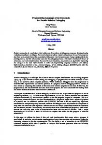
The bitonic merger is typically presented as a recursive construction and we have earlier explored ways to describe and analyse it in both (our) Ruby and in Lava [6, 14]. Here, we consider iterative descriptions using similar combinators. Figure 1 illustrates the merger for 16 inputs. Data flows from left to right. The vertical lines indicate components that operate on two array elements, placing the minimum onto the lower (abstract) wire, and the maximum onto the other output of the component.

Figure 1. A diagram of a 16 input bitonic merging network, using a style that is standard in the literature. Note that in each stage containing 8 min/max or comparator components, all 8 operate on independent parts of the input and so can proceed in parallel. The leftmost stage operates (for n = 16) on elements that are 8 apart. the next stage deals with elements that are 4 apart, and so on. We introduce a combinator ilv1, for interleave, that captures this pattern. ilv1 i f g applies f to elements 2i apart, producing the output at the lower of the two input indices; it applies g to the same pairs of elements, producing the output on the upper index. Defining stage i to be ilv1 i min max, the four stages in the diagram are simply stage applied to3, 2 1 and 0. The definition of ilv1 makes use of the fact that flipping the bit i of an index (using the function flipBit) gives the index of the element that will be combined with it using the functionsf and g. The decision about whether to apply f or g is made by looking at the value of bit i. As we shall see, the use of the Obsidian ifThenElse produces conditionals in the resulting CUDA. lowBit :: Int -> UWordE -> Exp Bool lowBit i ix = (ix .&. bit i) ==* 0 flipBit :: Bits a => Int -> a -> a flipBit = flip complementBit ilv1 :: Choice a => Int -> (b -> b-> a) -> (b -> b -> a) -> Array b -> Array a ilv1 i f g arr = Array ixf (len arr) where ixf ix = let l = arr ! ix r = arr ! newix newix = flipBit i ix in (ifThenElse (lowBit i ix) (f l r) (g l r))

Expressing ilv1 using bit-flipping may seem strange, but it has the advantage that it actually applies the desired pattern of computation repeatedly over larger input arrays. Now, for 2n inputs, a Haskell list containing the n calls of this interleave combinator are built: bmerge :: Int -> [Array IntE -> Array IntE] bmerge n = [istage (n-i) | i [Array (Exp a) -> Array (Exp a)] -> Array (Exp a) -> Kernel (Array (Exp a)) compose = composeS . map pure runm k = putStrLn$ CUDA.genKernel "bitonicMerge" (compose (bmerge k)) (namedArray "inp" (2^k))

Note that bmerge k works on inputs of length 2k+j , for j > 0, applying the merger to sub-sequences of length 2k . The CUDA code for bmerge 4 on 16 inputs (with some newlines inserted) is *Main> runm 4 __global__ void bitonicMerge(int *input0,int *result0){ unsigned int tid = threadIdx.x; unsigned int bid = blockIdx.x; extern __shared__ unsigned char sbase[]; (( int *)sbase)[tid] = ((tid&8)==0) ? min(input0[((bid*16)+tid)],input0[((bid*16)+(tid^8))]) : max(input0[((bid*16)+tid)],input0[((bid*16)+(tid^8))]); __syncthreads(); (( int *)(sbase + 64))[tid] = ((tid&4)==0) ? min((( int *)sbase)[tid],(( int *)sbase)[(tid^4)]) : max((( int *)sbase)[tid],(( int *)sbase)[(tid^4)]); __syncthreads(); (( int *)sbase)[tid] = ((tid&2)==0) ? min((( int *)(sbase+64))[tid],(( int *)(sbase+64))[(tid^2)]) : max((( int *)(sbase+64))[tid],(( int *)(sbase+64))[(tid^2)]); __syncthreads(); (( int *)(sbase + 64))[tid] = ((tid&1)==0) ? min((( int *)sbase)[tid],(( int *)sbase)[(tid^1)]) : max((( int *)sbase)[tid],(( int *)sbase)[(tid^1)]); __syncthreads(); result0[((bid*16)+tid)] = (( int *)(sbase+64))[tid];

3.3 Modifying the bitonic merger The bitonic merger for which we have just generated a kernel is known to sort so-called bitonic sequences, which include sequences whose first half is sorted in one direction and whose second half is sorted in the other direction. This fact can be used to build the wellknown bitonic sorting network. However, a GPU implementation typically needs to check, for each comparator, whether or not it should sort upwards or downwards, see for instance the simple CUDA implementation shown in Appendix A. We choose here to modify the merger so that it sorts two concatenated sequences that are sorted in the same direction. We do this by using a wellknown trick, reversing half of the input to the merger. It turns out that we can also reverse the same half of the output of the first stage of the network, without affecting overall behaviour. The resulting network, tmerge, shown in Figure 2, encourages us to develop a new combinator to describe the characteristic V-shaped pattern that results in the first stage. The combinator is modelled on ilv1. The only difference is that the “partner” of an index is found not by flipping bit i, but by flipping bits 0 to i, using function flipLSBsTo. The implementation of vee1 is got from that for ilv1 by replacing the call of flipBit by one of flipLSBsTo (and we could also have chosen to make a more generic function that is parameterised on this partner function). flipLSBsTo :: Int -> UWordE -> UWordE flipLSBsTo i = (‘xor‘ (oneBits (i+1))) vee1 :: Choice a => Int -> (b -> b-> a) -> (b -> b -> a) -> Array b -> Array a vee1 i f g arr = Array ixf (len arr) where ixf ix = let l = arr ! ix r = arr ! newix newix = flipLSBsTo i ix in (ifThenElse (lowBit i ix) (f l r) (g l r)) tmerge :: Int -> [Array IntE -> Array IntE] tmerge n = vstage (n-1): [istage (n-i) | i [Array IntE -> Array IntE] tsort1 n = concat [tmerge i | i UWordE) -> ArrayP a -> ArrayP a ixMap f (ArrayP p n) = ArrayP (ixMap’ f p) n ixMap’ :: (UWordE -> UWordE) -> P (UWordE, a) -> P (UWordE, a) ixMap’ f p = \g -> p (\(i,a) -> g (f i,a)) insertZero insertZero insertZero = a + (a

:: Int -> UWordE -> UWordE 0 a = a ‘shiftL‘ 1 i a .&. fromIntegral (complement (oneBits i :: Word32)))

ilv2 :: Choice b => Int -> (a -> a -> b) -> (a -> a -> b) -> Array a -> ArrayP b ilv2 i f g (Array ixf n) = ArrayP (\k -> app a5 k *>* app a6 k) n where n2 = n ‘div‘ 2 a1 = Array (ixf . left) (n-n2) a2 = Array (ixf . right) n2 a3 = zipWith f a1 a2 a4 = zipWith g a1 a2 a5 = ixMap left (push a3) a6 = ixMap right (push a4) left = insertZero i right = flipBit i . left app (ArrayP f _) a = f a

This new combinator can now replace ilv1 in the bitonic merger, giving a kernel that runs considerably faster. We will use that kernel to build a large sorter later. The implemenation of vee2 is almost identical to that of ilv2, with flipBit i replaced by flipLSBsTo as before (so that, again, one would in fact make a more generic function for building such combinators). Now, we just need to replace the ilv1 and vee1 combinators in the tree sorter with ilv2 and vee2 , to get a verrsion that uses half as many threads: tmerge2 :: Int -> [Array IntE -> ArrayP IntE] tmerge2 n = vstage (n-1) : [ istage (n-i) | i [Array IntE -> ArrayP IntE] tsort2 n = concat [tmerge2 i | i [Array IntE -> ArrayP IntE] bpmerge2 n = [vstage (n-i) | i Int -> Int -> a -> a flipBitsFrom i j a = a ‘xor‘ (fromIntegral mask) where mask = (oneBits (j + 1):: Word32) ‘shiftL‘ i ilvVee1 :: Choice a => Int -> Int -> (b -> b-> a) -> (b -> b -> a) -> Array b -> Array a ilvVee1 i j f g arr = Array ixf (len arr) where ixf ix = let l = arr ! ix r = arr ! newix newix = flipBitsFrom i j ix in (ifThenElse (lowBit (i+j) ix) (f l r) (g l r)) ilvVee2 :: Choice b => Int -> Int -> (a -> a -> b) -> (a -> a -> b) -> Array a -> ArrayP b ilvVee2 i j f g (Array ixf n) = ArrayP (\k -> app a5 k *>* app a6 k) n where n2 = n ‘div‘ 2 a1 = Array (ixf . left) (n-n2) a2 = Array (ixf . right) n2 a3 = zipWith f a1 a2 a4 = zipWith g a1 a2 a5 = ixMap left (push a3) a6 = ixMap right (push a4) left = insertZero (i+j) right = flipBitsFrom i j . left app (ArrayP f _) a = f a

For both variants of the combinator, we simply add to the ilv definitions a new Int parameter, j, and replace flipBit i by flipBitsFrom i j. We also insert the zero bit (when calculating the left index) at position i + j rather than just at position i. ilvVee is a generalisation of both ilv and vee. ilvVee i 0 has the same behaviour as ilv i, and ilvVee 0 (j-1) is the same as vee j. The i parameter controls the degree of interleaving, and the j parameter controls the size of the vee-shaped blocks. For 16 inputs, the parameters to ilvVee that describe the periodic merger on the right of the construction are i = 0 (for no interleaving) paired with 3, 2, 1 and 0 for the decreasing size of

tt

Figure 5. A sorter based on the idea that the periodic balanced merger network sorts two interleaved sorted sequences. It consists of two half-sized sorters, one working on the odd elements of the input and one on the even, followed by the balanced merger. The diagram indicates using dotted lines the balanced merger that is the final (rightmost) part of one of the half-size sorters. unsigned unsigned unsigned unsigned

int int int int

arrayLength = 1