Extending Hough Transform to a Points’ Cloud for 3D-Face Nose-Tip Detection Vitoantonio Bevilacqua1,2, Pasquale Casorio1, and Giuseppe Mastronardi1,2 1
Dipartimento di Elettrotecnica ed Elettronica Politecnico di Bari Via Orabona, 4 70125 - Bari - Italy
[email protected] 2 e.B.I.S. s.r.l. (electronic Business in Security), Spin-Off of Polytechnic of Bari, Str. Prov. per Casamassima Km. 3-70010 Valenzano (BA)-Italy
Abstract. This paper describes an extension of Generalized Hough Transform (GHT) to 3D point cloud for biometric applications. We focus on the possibility to applying this new GHT on a dataset representing point clouds of 3DFaces in order to obtain a nose-tip detection system.
1 Introduction In Computer Vision object or shape detection in 2D/3D images is very hard to solve because shapes can be subject to translations, can change by color, can be subject to scale and orientation, can endure occlusions and moreover data acquisition can introduce high levels of noise. One of the more effective solutions for shape detection is the Hough Transform. Formulated for the first time in early ‘60s, it originally was able to recognize shapes that had analytical description such as straight lines, circles and ellipses in 2D intensity images. In 1981 Ballard [1] proposed an extension defined Generalized Hough Transform (GHT) for generic shape detection by using the R-Table, a table that describes the shape to search respect to a reference point that could represent the center of the pattern. Many efforts have been done in order to try to extend the GHT in threedimensional images. Khoshelham [2] proposed an extension of Ballard GHT for three-dimensional images constituted by point clouds obtained by means of laserscanner acquisitions, for generic applications. This work adapts Khoshelham GHT in an attempt to apply it on 3D-Face shaded model for nose-tip detection. In this way it is possible to create an automatic repere’s points detection system with the purpose of obtaining a biometric system for AFR (Automatic Face Recognition) using 3DFace templates. The research was lead on a database of 3D-faces in ASE format, the GavaDB, given by the GAVAB research group of computer science department at the University of King Juan Carlos in Madrid. D.-S. Huang et al. (Eds.): ICIC 2008, LNAI 5227, pp. 1200–1209, 2008. © Springer-Verlag Berlin Heidelberg 2008
Extending Hough Transform to a Points’ Cloud for 3D-Face Nose-Tip Detection
1201
2 An Overview of the Standard and Generalized Hough Transform 2.1 The Standard Hough Transform The idea of Hough transform for detecting straight lines in2D intensity images was first introduced by Hough in 1962. It uses the Hesse normal form to represent a straight line:
Fig. 1. The straight line and its Hesse normal form parameters
ρ = X cos θ + Y sin θ
(1)
The parameters ρ and θ represent the distance of the application point of the normal vector from the origin of XY reference system, and the angle that it forms with the X-axis. In this way it is possible to consider a transformation from the plan of the image (on which the shape it is represented) to the space of the parameters: • A straight line in XY space corresponds to a point (ρ’, θ’) in the parameter space. • Each pixel in the image corresponds to a curve representing all the parameters of the lines of a bundle of straight that have that pixel as intersection point . • Fixing two pixels, they identify one and one single straight. Such situation is represented in the space of the parameters by means of an intersection of the curves correspondents to the same points. The parameter space is realized in the form of a discrete accumulator array H[θ][ρ], consisting of a number of bins that receive votes from edge pixels in the image space. The algorithm will be: • • • • •
Bound ρ and θ in order to obtain 2 2 0 ≤ ρ ≤ Max, 0 ≤ θ ≤ 2π, where Max=0,5·√(NPixelRow +NPixelColumn ) Choose the level of accumulator array quantization basing on the desired accuracy. Annul the H array. For each pixel P having coordinates (x, y) - for θn in [0, 2π] with step dθ 1. Evaluate ρ(n)=x·cos(θn)+y·sin(θn) 2. Obtain the index m that corresponds to ρ(n) 3. Increase H(m,n) of one vote. - End • End
1202
V. Bevilacqua, P. Casorio, and G. Mastronardi
Find straight lines parameters corresponding to the accumulator bins that received the most numbers of votes. 2.2 The GHT Proposed by Ballard [1] The standard Hough transform is only able to detect shapes described by parametric equations. However, in real applications the pattern to detect can be so complex than it could not be represented by any analytic description. In 1981, D. H. Ballard proposed a HT extension for generic shape detection.
Fig. 2. Example of pattern and equations involved in Ballard’s method
We can arbitrary choose a reference point (Xc, Yc) representing the centre of the pattern, and several points (X, Y) on the shape edge. The angle Φ that the tangent line forms at the edge point with the X axis, represents towards of route of the edge. Each edge point can be described by an ordered couple such as (r, α) like figure 2 suggests. Now, if a (X, Y) pixel image is an edge point of a pattern centered in (Xc, Yc), it satisfies the equation (2):
⎧ X c = X + r cosα ⎨ ⎩ Yc = Y + r sin α
(2)
All the couples (r, α) can be written in a table, called R-Table, sorting them in order to each row contains all the couple which have the same Φ value.
Extending Hough Transform to a Points’ Cloud for 3D-Face Nose-Tip Detection
φ1 : φ2 : ...
φn :
(r , α ), (r (r , α ), (r 1 1 2 1
(r
1
1 1 2 1
1 2 2 2
...
n
,α
n 1
), (r
n 2
1203
) ),...
, α 21 ,... ,α
2 2
)
, α 2n ,...
Fig. 3. Example of R-Table
The GHT algorithm is: • The parameters space that is represented by accumulator array H, corresponds to XY coordinates of the reference point (pattern centre). Quantization level is chosen in order to obtain the desired accuracy level. Initially each accumulator bin is null. • For each image’s pixel (Xp, Yp) to examine evaluate Ф angle and research the R-Table row indexed by its quantization. • For each couple (r, α) found in the R-Table , calculate - xc = xp + r cos α yc = yp + r sin α - Increase H[Xc][Yc] of one vote. • Find the most voted bins. They represent the centre points where shape occurrences are localized into the image. • If needed, using the centers obtained in previous step to rebuild the pattern as visual reply.
3 The GHT for 3D-Point Clouds by Khourosh Khoshelham [2] The Generalized Hough Transform is larger employed because of : • It transforms shape detection problem (very hard to solve) into a maximum analysis problem, that is simpler and simpler than the original one. • It is robust to partial or slightly deformed shapes (i.e., robust to recognition under occlusion). • It is robust to the presence of additional structures in the image (i.e., other lines, curves, etc.). • It is tolerant to noise. • It can find multiple occurrences of a shape during the same processing pass. • However, these advantages are not “free of charge”, in fact: • We need to build a separate R-table for each different object. • It requires a lot of storage and extensive computation (but it is inherently parallelizable!). If we want to include pattern scale and rotation, it is necessary to add these parameters to the accumulator array, and the computational cost could become too high.
1204
V. Bevilacqua, P. Casorio, and G. Mastronardi
All the HT and GHT have been created for shape detection in two-dimensional images. One of most interesting challenges consists of obtaining a GHT model to detect patterns in 3D-images, i.e. point clouds, representing objects acquired by means laser scanner. K. Khoshelham proposed a GHT model that we can consider as Ballard’s GHT extension for 3D-images. Considering an arbitrary three-dimensional pattern (figures 4 and 5), the edge is by a generic surface. Edge vertex normal vectors could give information about towards of route of the surface such as Φ angle does in Ballard’s GHT.
Fig. 4. Example of a generic pattern
Fig. 5. Parameters involved in R-Table build process
The algorithm of R-Table creation can therefore be modified: • Examine all the pattern vertexes choosing a centre as reference point. This one will be randomly chosen. A method could consist of evaluate the mean values of pattern’s vertexes coordinates. • Evaluate for each point P of the pattern a. r = ( X c − X p ) 2 + (Yc − Yp ) 2 + ( Z c − Z p ) 2 ⎛ Z − Zp ⎞ ⎟⎟ b. α = cos −1 ⎜⎜ c ⎝ r ⎠ −1 ⎛ X c − X p ⎞ ⎟⎟ c. β = cos ⎜⎜ ⎝ r sin α ⎠
(3)
[Both α and β in [0, π] ] - Evaluate vertex normal vector angles ψ and φ, and quantize them in order to obtain the R-Table indexes. • Insert the tern (r, α, β) into the R-Table shown in Figure 6.
Extending Hough Transform to a Points’ Cloud for 3D-Face Nose-Tip Detection
1205
Fig. 6. Example of 2D R-Table
The algorithm consists of these steps: • Build the accumulator array H and null it. The accumulator represents the X, Y and Z coordinates of the pattern center in the point cloud. • Read and store in memory the accumulator array H. • For each point of the cloud to examine: - Evaluate its normal vector angles and quantize them in order to obtain the RTable indexes. - For each tern (r, α, β) extracted using previous indexes: • Evaluate ⎧ X c = X p + r sin α cos β ⎪ ⎨ Yc = Yp + r sin α sin β ⎪ Z c = Z p+ r cos α ⎩
(4)
• Increase H[X’c][Y’c][Z’c] of one vote. X’c, Y’c and Z’c represent the quantized values of centre coordinates . • Find the center coordinates corresponding to the accumulator bins that received the most numbers of votes. • If needed, using the centers obtained in previous step to rebuild the pattern as visual reply. If we want to consider geometric transformations such as rotation and scale involving the pattern in the point cloud, the algorithm may be modified. Equation (4) should be changed with (5), express in vector form: c=p + s MzMyMxr
(5)
Where: T
c := (Xc, Yc, Zc) p := (Xp, Yp, Zp)T T r := ( r sin(α )cos(β ), r sin(α )sin(β ), r cos(α ) ) s := scale factor Mz, My, Mx := axis rotation matrixes. These changes lead the accumulator array to be 7-dimensional array. Three dimensions represent the centre coordinates, one dimension represents the scale factor, and the other three ones represent the rotation along the X, Y and Z axis. So, voting process will generate both rotational and scale factor values by attempts.
1206
V. Bevilacqua, P. Casorio, and G. Mastronardi
However, this solution remains theoretical because of its very high computational costs. Our first 3D-GHT application implements the original algorithm, without scale and rotation, and even in this simpler case the accumulator array uses about 200MB of RAM for memory allocation, to obtain the desired accuracy. The algorithm takes about 10 seconds to detect shapes in point clouds consisted of ten thousands vertexelements. Our second 3D-GHT application improves previous version implementing pattern scale by means a simplified version of equation 5: c=p + s r
(6)
A “for-loop” fixes the scale factor before evaluating equation 6. So, it uses an [331]x[331]x[331]x[8] accumulator array. Fourth dimension represents scale factor. With a scale factor’s step of 0.25, the algorithm is able to find 3D-shapes which are in dimensions from 0.25 to 2 times original pattern’s ones. This algorithm uses about 1GB of RAM and takes less than 20 seconds to detect shape in point clouds consisted of ten thousands vertex-elements. Concerning time complexity, all the HT algorithms are O(N), where N represents the number of point cloud’s vertexes.
4 The 3D GHT at Work on 3D Faces The first GHT application (without pattern scale) was tested on a 3D-Face database. Faces have been acquired with different poses. The patterns were spheres with beams of 3.5, 4 or 5 (adimensional values). Maximum analysis demonstrated how most voted sphere with 3.5 and 5 beams were next to the nose in 80% of examined faces. This result was used to create an automatic nose-tip detection application. Nosetip, in fact, is the most important repere point, and it is used in biometrics as parameter in order to study face symmetry or face recognition by means repere points’ triangulation. The research algorithm can be described by these steps: 1. Research the most voted 3.5 beam sphere. In case of fault, a 5 beam sphere is used. The beams are adimensional values because is impossible extracting from the database information about scale factor involved in data acquisition. 2. Extract face vertexes in proximity of the found sphere, magnifying extracted cloud of a factor of 10. 3. Research the most voted 5 beam sphere on the cloud extracted in the previous step, in order to center the sphere on the nose. 4. Evaluate the mean value of normal vectors of each face vertex with the purpose of obtaining information about face orientation in the three-dimensional space. 5. Move the center of the sphere by the direction evaluated in step 4, and proportionally to the sphere beam value. In this way we collapse the entire sphere in a point that represents the nose-tip. 6. The point that we obtained in step 5 may not be present among the vertex of the examined face. So the last step consists to research the closest face vertex to the nose-tip previously extracted. This vertex represents the real nose-tip.
Extending Hough Transform to a Points’ Cloud for 3D-Face Nose-Tip Detection
1207
Fig. 7. Example of using 3D-GHT (without pattern scale) to extract nose vertex from a 3DFace point cloud
Second GHT algorithm was tested with the same 3D-Faces database using only a 3.5 beam sphere as pattern. In this case, the application was able to find spheres with beam of 0.875, 1.75, 2.625, 3.5, 4.375, 5.25, 6.125 and 7. Maximum analysis demonstrated how scale factor introduces in our results both accuracy and new spheres, so the ones next to the nose were not the most voted anymore. We had to consider a different nose-tip research algorithm (it works only if the point cloud represents a frontal face or lightly rotated one) : 1. Calculate mean value of face vertexes; 2. Extract face vertexes that are in a hypothetic sphere of beam 13 (was the value that gave us best results). This sphere is centered in XYZ point calculated in the previous step. 3. Using the latest GHT application with vertexes at step 2 with 1 as threshold value. 4. Evaluate the mean value of normal vectors of each face vertex with the purpose of obtaining information about face orientation in the three-dimensional space. 5. Move the center of the sphere by the direction evaluated in step 4, and proportionally to the sphere beam value in order to collapse the entire sphere in a point that represents the nose-tip. 6. The point that we obtained in step 5 may not be present among the vertex of the examined face. So the last step consists to research the closest face vertex to the nose-tip previously extracted. This vertex represents the real nose-tip. 4.1 Results 18 3D-Faces have been verified. In table 1 we report nose-tip XYZ coordinates calculated by means both algorithms. As shown in table 1, only in three cases both the algorithms find the same vertex. In other ones, except for faces 2, 3,5 and 14, for each face vertexes found by the algorithms are next each other and both represent a good approximation of nose-tip repere point. Regarding face 5 the second algorithm gives a better result and in face 7
1208
V. Bevilacqua, P. Casorio, and G. Mastronardi
Table 1. Main Results. Note: Coordinates marked with (B) are better in accuracy than coordinates calculated with our other algorithm.
Face
1 2 3 4 5 6 7 8 9 10 11 12 13 14 15 16 17 18
Points’ GavaDB ASE File Cloud (Face Source) File* V1-1.txt Face01-1.ASE V1-2.txt Face01-2.ASE V1-4.txt Face01-4.ASE V2.txt Face02-9.ASE V3.txt Face03-4.ASE V4.txt Face04-4.ASE V5.txt Face05-4.ASE V6.txt Face06-4.ASE V7.txt Face07-4.ASE V8.txt Face08-4.ASE V9.txt Face09-4.ASE V10.txt Face10-4.ASE V11-1.txt Face11-1.ASE V11-8.txt Face11-8.ASE V12.txt Face12-5.ASE V13.txt Face13-4.ASE V14.txt Face14-8.ASE V15.txt Face22-5.ASE
Nose-tip XYZ Vertex Coordinates Research through Research through GHT GHT w/o Scale w/ Scale 0.006 -22.914 -556.300
0.006 -22.109 -556.696 4.186 -2.494 -567.121 -10.629 -13.029 -553.1(B) -10.644 -11.419 -554.106 (0.006 -7.724 -545.446)** 0.841 -0.829 -566.700(B)
-92.434 -3.733 -455.800
-95.169 -3.728 -455.350(B)
-11.747 -6.092 -516.200
----------92.329 2.590 -548.000
-12.402 -5.442 -515.991 -95.016 -18.058 -550.200 -92.334 1.940 -547.645
-100.244 -19.925 -541.000
-101.039 -19.120 -540.675
-93.292 -8.210 -558.300
-92.462 -9.035 -558.585 -125.189 -18.885 -462.325
-126.019 -20.540 -461.60 -124.921 -14.981 -534.10
-125.716 -16.545 -533.770
-147.417 -26.840 -528.30
-147.417 -27.630 -528.495
-110.734 -4.060 -552.0(B)
-109.919 -2.435 -551.945 -128.377 0.005 -518.200 -128.372 0.765 -517.925 (-93.656 1.597 -534.485)** (-80.260 -26.165 -536.010)** -8.454 -6.889 -518.800 -8.449 -6.119 -518.636
*(Both the algorithm use pre-processed points’ clouds but in different steps. So we refer to original points’ clouds extracted from ASE file associated). **(Both the algorithms have extracted the same vertex).
is able to find nose-tip vertex against failure by the one without scale factor. Considering that the latest research algorithm uses just one GHT run (while the previous version uses two GHT runs), saving about 10 seconds of execution time, we can say we had a good improvement if RAM needed does not represent a problem.
Fig. 8. 3D views of some results: Face 7, Face 9 and Face 11. The subjects are shown in original pose.
Extending Hough Transform to a Points’ Cloud for 3D-Face Nose-Tip Detection
1209
5 Conclusions and Future Works This paper described how we extended Hough Transform for three-dimensional point clouds regarding 3D-face models, and how this GHT can be used in nose-tips detection with good results. Future work will be lead on: 1. The 3D-GHT, with the purpose of obtaining a low-cost algorithm including pattern rotation. 2. Biometrics applications, combining the 3D-GHT with face geometry in order to improve our nose-tip detection method. 3. Using 3D-GHT to detect other repere point, so as to create a complete AFR System.
References 1. Ballard, D.H.: Generalizing the Hough Transform to Find Arbitrary Shapes. CVGIP 13, 111–122 (1981) 2. Khoshelham, K.: Extending Generalized Hough Transform to Detect 3D Objects in Laser Range Data. Optical and Laser Remote Sensing Research Group, Delft University of Technology, Kluyverweg 1, 2629 HS Delft, The Netherlands; ISPRS Workshop on Laser Scanning 2007 and SilviLaser 2007, Espoo, September 12-14, Finland (2007) 3. Peternell, M., Pottmann, H., Steiner, T., Transform, H.: Laguerre: Geometry for the Recognition and Reconstruction of Special3D Shapes. Institute of Geometry, Vienna University of Technology, Vienna, Austria September 5 (2003)