EXTENDING THE COMPUTATIONAL HORIZON - Semantic Scholar

EXTENDING THE COMPUTATIONAL HORIZON: EFFECTIVE DISTRIBUTED RESOURCE-BOUNDED COMPUTATION FOR INTRACTABLE PROBLEMS∗

Harry J. Paarsch Department of Economics University of Iowa and Alberto M. Segre Department of Management Sciences and Department of Computer Science University of Iowa

May 1999

Abstract A number of combinatorial search problems of interest to computational economists belong to the complexity class NP. The best known solutions to these problems require computation times which are at least exponential in the size of the input; this renders many applications intractable. We present an overview of a new distributedcomputating technique called “nagging,” which potentially allows one to solve large exponential-time problems by efficiently exploiting multiple processors. Nagging requires relatively infrequent and brief communication among processors, so it is both naturally fault tolerant (unaffected by the dynamic loss of processing elements) and robust to high message latencies. Thus nagging is exceptionally scalable, making it useful in very large networks. ∗ We are grateful to M. Ryan Haley for helpful comments and useful sugges-

tions.

1.

Introduction and Motivation

Much of what economists do involves optimization. Typically economists constrain themselves to finding the maximum (minimum) of a concave (convex) C2 function on a convex set. Optima of such functions can be characterized in terms of first- and second-order conditions derived using the calculus. Failing closed-form solutions, a wide variety of algorithms (e.g., Newton’s method) can be used to approximate the solutions to such problems. Computer scientists have created a theory for describing the difficulty of computational problems in terms of the time requirements of their solutions.

For example, hill-climbing algorithms based on the derivatives of C 2

concave functions are polynomial-time algorithms: as the number of variables k involved in the optimization increases, the worst-case time to find a solution is a polynomial in k. If, for a particular algorithm, the highest order of this polynomial is p, then the algorithm is said to be of order k p , denoted O(k p ). Different algorithms may have the same asymptotic order, but their performances can differ greatly. By constraining themselves to concave C2 functions on convex sets economists limit the number of potential solutions that must be considered. This speeds up finding an optimum, but at the cost of considering only a subset of all feasible points. For some applications these assumptions are good approximations, for others they are not. A wide variety of optimization problems requires complete enumeration of all points in the space of alternatives rather than just examining points which satisfy the first-order conditions. Some two-sided matching problems in economics, the travelling-salesman’s problem in operations research, and protein-folding problems in biology are concrete examples of problems with this structure; see Roth and Sotomayor (1990) for two-sided matching problems, Winston (1994) for travellingsalesman’s problems, and Atkins and Hart (forthcoming) for protein-folding problems. These problems differ from problems that have polynomial-time solutions in structural ways. Combinatorial search problems belong to the complexity class known as NP, for “nondeterministic polynomial time.” Problems within this complexity class share an important characteristic: while the best known solutions to these problems require at least exponential time, verifying that a solution is indeed the 1

optimum requires only polynomial time. Note that whether better-than exponentialtime solution algorithms exist is still an open problem, although it is widely believed that no such solutions will be found.1 Just because a problem requires an exponential-time solution algorithm does not mean the problem is uninteresting. Many such problems are of great practical importance. What complexity theory implies, however, is that for all such problems a “computational horizon” exists, beyond which solutions are difficult to obtain in reasonable time. One obvious way of extending the computational horizon is to apply multiple computing elements in tandem: parallel computing. With the increased availability of large laboratories of powerful desktop personal computers, solving large computational problems in parallel has become economically feasible. Unfortunately, parallelizing large problems is difficult. The traditional approach to solving a problem in parallel typically involves partitioning the problem into smaller problems (subproblems) and then joining the solutions of these subproblems to generate a solution to the original problem. Partitioning can be done using two or more subproblems and can sometimes occur recursively. Elegant partitioning of any computational problem is tricky; one must be respectful of both load balancing and potential processor-failure. To balance loads properly on several computers requires some notion of how computationally intensive each partition is. Also, in a distributed-computing system of any reasonable size the probability of some machine’s failing is high; a useful computational approach must be robust to these failures, also referred to as fault tolerant. With many processors the fixed costs arising from communication among processors, often referred to as overhead, becomes important. Keeping communication to a minimum is central to reaping any advantages from parallelism. Partitioning NP problems is particularly difficult for several reasons. First, load 1 A large class of decision-theoretic problems within the NP class (i.e., those that only require a yes/no solution) are said to be “NP complete.” This essentially means that finding a polynomial-time solution algorithm for one of these problems will also yield a polynomialtime solution for all of the other problems in this complexity class. Problems within this complexity class stand or fall together.

2

balancing is hard to do because one does not know a priori the sizes of subproblems. Next, solving subproblems concurrently precludes using information from one subproblem to help solve another; even if one could make use of partial-solution information from other subproblems the communications costs would become prohibitive. Finally, intuitively, if there were a good partitioning approach to solving NP problems, then such problems would not be NP: problems amenable to partitioning are those for which the divide-and-conquer strategy applies. Algorithms based on a divide-andconquer strategy are generally polynomial-time algorithms. Thus, in practice, using partitioning to exploit multiple processing elements is extraordinarily difficult for this class of problems. Nagging is a novel technique for search in a distributed-computing environment. Nagging requires relatively infrequent and brief communication among processors making it both naturally fault tolerant (unaffected by the dynamic loss of processing elements) and robust in the presence of high message latencies. Thus nagging is exceptionally scalable and particularly useful in very large networks. A computational technique like nagging cannot bypass the exponential-time, worst-case solution structure inherent in the complexity class NP. On average, nagging reduces the base on the exponential term in the solution-time analysis, leading to faster solutions in practice. Nagging can lead to superlinear speedups for some difficult problems. Nagging scales well to many processors. Hence it is particularly apt at solving very large problems without loosing speed. 2.

Nagging: A Distributed Adversarial Search-Pruning Technique

In many ways nagging is the dual of partitioning: instead of subdividing a problem, nagging concurrently explores alternative representations of the problem to find the solution to each individual subproblem more quickly. Two types of processes are used: a master process, which attempts to solve a problem via a standard sequential-search procedure, and one or more nagging processes. Each nagging process, when idle, simply selects a portion of the master’s current search space and explores it in parallel, subject to the solution constraints to which the master has already committed. If the 3

nagger finds a solution, then the master will also eventually find the same solution. On the other hand, if the nagger exhausts its search space without finding a solution consistent with the current set of solution constraints, then it is clear the master’s current search is irrelevant because it can never lead to a global solution. Here the nagger interrupts the master, forcing it to backtrack and resume its search at a point where a solution remains feasible. This “pruning” contributes to the reduction in the master’s search effort; see Sturgill (1996) as well as Sturgill and Segre (1997). For a nagger to contribute to the search efficiently it must be able to exhaust its search space faster than the master processor. Ensuring this requires a problem transformation function (PTF). Intuitively, a PTF recasts the original search problem as a different search problem in the hope that, on average, the recast problem will be solved faster. A transformed problem space is simpler if it has a solution whenever the original one does; it can also contain some extraneous solutions. Another important property of a “simpler” problem space is that it should be smaller. If the nagger fails to find a solution in the smaller transformed space, then one can safely assume no solution exists in the original space.2 An example, which will also form the basis of our computational experiments, should make this clear. Consider the classical Euclidean travelling-salesman’s problem (TSP) which is known to belong to the complexity class NP; i.e., no less than an exponential-time solution is known (or expected) to exist. In the example described below we shall use a na¨ıve exponential-time algorithm to illustrate how nagging works.3 Consider a set of k cities {C1 , C2 , . . . , Ck } located in the Euclidean plane. We seek an ordering of these k cities which yields the shortest tour among the cities without repeat {S1 , S2 , . . . , Sk } where Si is a member of {C1 , . . . , Ck } with no Si equalling Sj for all i not equal to j. A graphical depiction of ten cities and a potential tour is illustrated in Figure 1. 2 Another technique that helps ensure a nagger exhausts its space more quickly than the master is to nag recursively the nagger with additional processors. 3 We chose the TSP because it is easy to explain and to understand. We do not exploit the special structure of the TSP. In practice the TSP can be solved quickly using a variety of heuristics which exploit the problem’s special structure.

4

Figure 1 Potential Tour in Ten-City TSP

1

5 6 7

2 4

3

8

9 10

Figure 2 Tree of Potential Tours for TSP 123

1234

12345

1243

12354

12534

15234

152346

152364

152634

5

156234

1423

165234

Beginning with a randomly-selected triad of cities (without loss of generality choose C1 , C2 , and C3 ) we attempt to insert each successive city into the partial tour at every possible location. Thus (C1 , C2 , C3 ) becomes (C1 , C2 , C3 , C4 ) or (C1 , C2 , C4 , C3 ) or (C1 , C4 , C2 , C3 ); see Figure 2. Continuing in this fashion enumerates all possible tours because exactly (k!/2) leaves exist and because each tour is considered only once.4 By exploring the entire space one can easily find the shortest tour. Now consider a technique to reduce the number of tours examined. If one keeps track of the shortest tour known so far, then any partial tour (internal node of the tree in Figure 2) that exceeds this length cannot possibly lead to a completed tour which is shorter than the best tour found so far. In fact one can do better if one considers an admissible estimate of the remaining tour distance. We use the triangle inequality for Euclidean spaces to estimate the remaining tour distance; for more on this, see Nilsson (1971). Hence the subtree rooted there need not be considered any further: it can be pruned. To see why nagging works one needs to realize first that the order in which solutions are explored has a large effect on the number of leaves actually visited. If the leaves are generated in a monotonically decreasing order of length, then they will not be pruned at all. But if the leaves are generated in the reverse order, then a lot of pruning will occur; relatively few leaves will be examined. One cannot know a priori which ordering is best, but nagging, in its simplest form, exploits well the random reordering of the leaves. Take the one-nagger case. The idle processor (nagger) requests a snapshot of the master’s search space along with the length of the best tour found so far. A node on the master’s current path to the root of the tree is then selected at random by the nagger; call this the “nagpoint.” Next the nagger randomly permutes the branchgeneration ordering function and “races” the master using this transformed space. Three possible outcomes can obtain: 4 Only (k!/2) leaves need be considered because the routing problem is symmetric and tours are closed; i.e., it does not matter where one starts. Thus the sequences (C 1 , C2 , C3 , C4 ) and (C3 , C2 , C1 , C4 ) represent identical tours.

6

1. The master exhausts its space first, backtracking over the nagger’s selected nagpoint. When this happens the nagger is told to abandon its search and to select a new nagpoint. 2. The nagger finds a shorter solution in its space. Then the nagger informs the master of the new tour length, gives up its search, and asks for a new nagpoint. 3. The nagger finds no shorter solution; it interrupts the master and tells the master to backtrack past the nagpoint. For the first outcome the nagger contributes nothing to the search. Yet herein lies the secret to nagging’s fault tolerance: if the nagging processor were to fail, then the validity of the master’s search would be unaffected. For the second outcome the nagger’s new bound may help the master prune more effectively. The big gain comes with the third outcome. Here the nagger is functioning as a parallel search-pruning system telling (nagging) the master “where not to look.” If the PTF is very likely to permute the solution time, then the third outcome will be common. When the PTF does not permute the solution time, nagging will usually follow the first outcome and contribute little or nothing to reducing the master’s search-solution time. 3.

Some Theoretical Bounds concerning the Effects of Nagging

In this section we construct a simple probabilistic model from which some informative statistical bounds concerning the distributions of the solution times of the TSP using one processor and multiple processors under nagging can be derived. We assume that a mapping exists from the space of possible solutions to the real line. Thus, for a given processor and for a particular configuration, the solution time T is a random variable with cumulative distribution function FT (t). The basic idea behind nagging is that processors race to complete the task and the fastest one wins. For n independent and identical processors the theoretical distribution of the fastest processor (abstracting from faults and overhead) can be derived as follows. Define the solution time of the fastest processor to be Y = min(T1 , T2 , . . . , Tn ) 7

where Ti is the solution time for the ith of the n processors. Now FY (y), the cumulative distribution function of Y , is related to FT (y) via the following equations: [1 − FY (y)] = Pr(Y ≥ y) = Pr[(T1 ≥ y) ∩ (T2 ≥ y) ∩ . . . ∩ (Tn ≥ y)] =

n Y

(1) Pr(Ti ≥ y) (by independence)

i=1

= [1 − FT (y)]n

(by identicality).

Thus the natural logarithm of the survivor function of Y , log[1 − FY (y)], is proportional to the natural logarithm of the survivor function of the serial solution, log[1 − FT (y)], having slope n when nagging is working at the theoretical lower bound for speed. Of course the reality of processor communication and failure could invalidate the distributional bound. An alternative bound worthy of examination is the performance of a parallel process relative to the “average” time. Define An to be T divided by the number of processors. It is instructive to compare the quantiles of the nagging solution times with those of An , defined by FT (t/n). When nagging yields better than linear speed, often referred to as superlinear speedup, a q-q plot of quantiles of An on the abscissa versus the quantiles of the nagging solution times on the ordinate should lie below the 45◦ line. 4.

Experimental Evidence concerning Nagging to Solve the TSP

The design of the experiments which apply nagging to the TSP is as follows: for each problem we set k equal to twenty cities. The location of each city in the Euclidean plane was drawn from a a two-dimensional, uniform pseudo-random number generator; the indices of the initial triad of cities were then drawn at random from the discrete uniform distribution on the set {1, 2, . . . , k}; and the algorithm described in Section 2 was then used to solve for the shortest Euclidean path among the k cities. In the case of nagging we used two, four, and eight processors: one, three, and seven naggers plus a master processor. We replicated the procedure ten thousand times. 8

We also attempted our research with ks of ten, fifteen, and twenty-five. The results for the ten- and fifteen-city problems are not remarkably different from those for the twenty-city problems. With twenty-five cities the problems took an inordinately long time to solve and often had to be censored so that the rest of the experiments could continue. The experiments for the twenty-city problems took approximately a week of computing time, while the entire set of experiments required about five weeks of computing time. 4.1. Hardware and Software The experiments reported here are based on a C implementation of the TSP search algorithm described in Section 2, which is a version of the A* search algorithm; see Nilsson (1971). The algorithm starts with a randomly-selected partial tour of length three, the solution space is then explored by inserting each city in all possible permutations. Partial tours which are known not to lead to better solutions are pruned. For these experiments the NICE (“Network Infrastructure for Combinatorial Exploration”) distributed infrastructure, which has been developed explicitly to support nagging, was used to manage a pool of networked Unix workstations. While NICE has been previously used for experiments with roughly one hundred heterogeneous machines, the experiments reported here relied on eight identically-configured Hewlett-Packard C360 PA-RISC CPUs, each having 1GB of RAM, and all connected by 100GB/sec Ethernet. 4.2. Empirical Results from Nagging Experiments In constructing the empirical distribution functions (EDFs) necessary for the empirical survivor functions and estimates of the quantiles of the sampling distributions of interest we focussed on the total number of nodes visited before the optimum was found as a measure of solution time. We chose this measure as a proxy for elapsed solution time instead of using the system clock because it is not plagued by the round-off error induced by the granularity of the system clock, on the order of ten milliseconds. 9

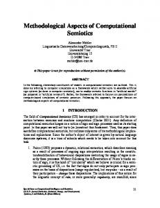
Figure 3 Processor Time versus Number of Nodes Visited Serial as well as Nagging with Two, Four, and Eight Processors 10

Natural Logarithm of Processor Time

9

8

7

6

5

4

3

2

4

6

8 10 12 Natural Logarithm of the Number of Nodes Visited

14

16

To see the effect of the round-off error induced in low-end solution times we graph in Figure 3 the natural logarithm of the number of nodes visited on the abscissa versus the natural logarithm of system-clock time on the ordinate. Notice that in the southwest corner of the graph a wide variety of node measurements yielded the same time on the system clock. Notice too the two distinct bands of points appearing in the northeast corner of the graph. These two bands arise because of the overheard per node (in milliseconds) that nagging introduces. The upper band of points corresponds to the nagging experiments, while the lower band of points corresponds to the serial experiments. This overhead arises because we used “flat” nagging, where idle processors only nag the master processor. This involves considerable redundant communication. In practice one would only use two or three naggers per master processor; additional idle processors would be used to nag the naggers. Flat nagging was 10

Figure 4 Natural Logarithm of Empirical Survivor Functions Serial versus Nagging with Two, Four, and Eight Processors

Natural Logarithm of Survivor Function of Nagging Solution Time

0

−2

y = x line

−4

n=2

−6

y = 2x line −8

n = 4, 8 −10

−12 −10

−9

−8 −7 −6 −5 −4 −3 −2 Natural Logarithm of Survivor Function of Serial Solution Time

−1

0

used because it is closer in spirit to equation (1). Note that the overhead measured is an upper bound; with fewer naggers and less redundant communication it would all but disappear. In Figure 4 we present a graph of the natural logarithm of the empirical survivor function of the serial solution time on the abscissa versus the natural logarithm of the empirical survivor functions for nagging with two, four, and eight processors. To help gauge the effect of nagging on the distributions of solution times we superimposed two lines, one for y = x and another for y = 2x. The “y = x” line frames the lower bound of improvement of nagging over the serial processor. The “y = 2x” line frames what the theoretical statistical relationship between log[1−FY (y)] and log[1−FT (y)] would be for two processors. Regressions of the logarithm of the empirical survivor functions of the nagging solution times for two, four, and eight processors on the logarithm of 11

Figure 5 q-q Plot of Natural Logarithm of Quantiles Linear Speedup versus Nagging with Two, Four, and Eight Processors

Natural Logarithm Quantiles of Nagging with 2, 4, and 8 Processors

20

18

16

14

n=8

n=2

12

10

8

6

n=4

4

2

0

0

2

4 6 8 10 12 14 16 Natural Logarithm Quantiles of Linear Speedup based on EDF of T

18

20

the empirical survivor function of the serial solution times yielded estimated slope coefficients of 1.3278, 1.5409, and 1.6203; all of the R2 s for these regressions were over 0.9945. Thus the independent-processor racing heuristic used to motivate the computational speedups through nagging appears overly optimistic; overhead due to initial startup and subsequently due to communication eats up a good portion of the potential gains. But can nagging attain superlinear speedups? In Figure 5 we graph the natural logarithm of the quantiles of the nagging solution times on the ordinate versus the natural logarithms of the quantiles of linear speedup on the abscissa. To calcuate the quantiles of linear speedup we used FˆT (t), the EDF of T , as an estimate of the true cumulative distribution function FT (t). We then estimated the quantiles of linear speedup using the inverse of the estimated cumulative distribution function Fˆ −1 (t/n) T

12

for n equal to two, four, and eight. The striking feature of Figure 5 is how close the nagging quantiles are to the linear speedup quantiles at low values as well as how, for long solution times, the quantiles move toward the 45◦ line, eventually falling below it at the high end of the solution-time distribution, where the startup costs are best amortized. These results are very encouraging because they suggest that nagging’s infrequent and brief use of interprocessor communication allows it to reap great benefits from computing in parallel, particularly for large problems where it is needed most. As mentioned the results for the ten- and fifteen-city solution times are basically the same. Not enough variation in k exists to make specific conclusions about the effect k has on the distributions of solution times with nagging. The twenty-fivecity solution times are difficult to summarize because of censoring due to inordinate amounts of computation time. In some sense this is unsurprising. In going from a twenty-city set of problems to a twenty-five-city set of problems there are 6, 375, 600 times as many potential solutions for each problem to examine and we are solving ten thousand problems. Given the evidence from Figure 5, however, it is in larger problems where nagging has the most potential. Economies of scale if you will. 5.

Summary and Conclusions

Combinatorial search problems are ubiquitous in real-world applications, including ones in economics. Because these problems belong to the complexity class NP the best algorithms can only provide exponential-time solutions. We have presented an overview of a novel computational technique, nagging, and evaluated its performance using experimental data for a class of TSPs. Nagging appears to provide near linear speedups in computation for small problems and potentially superlinear speedups for very large problems. With the advent of cheap hardware and the presence of large computing laboratories, which are often unused at night, nagging appears to hold promise for extending the computational horizon.

13

B. Bibliography Atkins, J. and W. Hart. “On the Intractability of Protein Folding with a Finite Alphabet.” Algorithmica, (forthcoming). Nilsson, N.. Problem-Solving Methods in Artificial Intelligence. New York: McGrawHill, 1971. Roth, A. and M. Sotomayor. Two-Sided Matching: A Study in Game-Theoretic Modeling and Analysis. Cambridge, UK: Cambridge University Press, 1990. Sturgill, D.. Nagging: A New Approach to Parallel Search Pruning. Ph.D. dissertation, Department of Computer Science, Cornell University, 1996. Sturgill, D. and A. Segre. “Nagging: A Distributed Adversarial Search-Pruning Technique Applied to First-Order Logic.” Journal of Automated Reasoning, 19 (1997), 347–376. Winston, W.. Operations Research: Applications and Algorithms. Third Edition. Belmont, CA: Duxbury, 1994.

14