Extending the Growing Neural Gas Classifier for Context Recognition Rene Mayrhofer1 and Harald Radi2 1
Lancaster University, Infolab21, South Drive, Lancaster, LA1 4WA, UK
[email protected] 2 Tumpenweg 528, 5084 Grossgmain, AT
[email protected]
Abstract. Context awareness is one of the building blocks of many applications in pervasive computing. Recognizing the current context of a user or device, that is, the situation in which some action happens, often requires dealing with data from different sensors, and thus different domains. The Growing Neural Gas algorithm is a classification algorithm especially designed for un-supervised learning of unknown input distributions; a variation, the Lifelong Growing Neural Gas (LLGNG), is well suited for arbitrary long periods of learning, as its internal parameters are self-adaptive. These features are ideal for automatically classifying sensor data to recognize user or device context. However, as most classification algorithms, in its standard form it is only suitable for numerical input data. Many sensors which are available on current information appliances are nominal or ordinal in type, making their use difficult. Additionally, the automatically created clusters are usually too fine-grained to distinguish user-context on an application level. This paper presents general and heuristic extensions to the LLGNG classifier which allow its direct application for context recognition. On a real-world data set with two months of heterogeneous data from different sensors, the extended LLGNG classifier compares favorably to k-means and SOM classifiers.
1
Introduction
Context Awareness, as a research topic, is concerned with the environment a user or device is situated in. Although its roots probably lie in robotics [1], the advantages of making applications in the fields of pervasive, ubiquitous or mobile computing aware of the user or device context are obvious: user interaction and application behavior can be adapted to the current situation, making devices and their applications easier to use and making more efficient use of the device resources. Our approach to making devices context aware is based on three steps: sensor data acquisition, feature extraction and classification [2]. In these three steps, high level context information is inferred from low level sensor data. There are two key issues in this approach: the significance of acquired sensor data, and the use of domain-specific heuristics to extract appropriate features. A broad view on
2
Rene Mayrhofer, Harald Radi
the current context is necessary for many applications, and can only be derived with a multitude of sensors with ideally orthogonal views of the environment. Using multiple simple sensors and merging their data at the classification step allows to use different heuristics for each sensor domain, and thus profit from well-known methods in the specific areas. Examples for simple sensors that are relevant to typical context-aware applications are Bluetooth or wireless LAN adapters, which can capture parts of the network aspect, the GSM cell ID, which defines a qualitative location aspect, or the name of the currently active application (or application part), which captures a part of the activity aspect of a user or device context. Other, more traditional sensors include microphones and accelerometers to capture the activity aspect [3], video cameras, or simple light and temperature sensors. The types of values provided by these sensors are very different. A method to cope with this heterogeneity of features has first been presented in [4] for the general case, independent of the used classification algorithm. This paper is concerned with necessary modifications to the Growing Neural Gas (GNG) classifier. GNG has been introduced by Bernd Fritzke in 1995 [5] and shares a number of properties with the conceptually similar Dynamic Cell Structure algorithm, which has been developed independently by Jörg Bruske and Gerald Sommer [6]. In 1998, Fred Hamker extended GNG to support life-long learning, addressing the Stability-Plasticity Dilemma [7]; the resulting algorithm has also been called Lifelong Growing Neural Gas (LLGNG). The main difference between GNG and LLGNG is that the latter uses local error counters at each node to prevent unbounded insertion of new nodes, thus allowing on-line learning for arbitrary long periods. The basic principle of GNG and LLGNG is to insert new nodes (clusters) based on local error, i.e. it inserts nodes where the input distribution is not well represented by clusters. For classification of features to recognize context, this is an important property because it ensures independence of the usually unknown input distribution. Additionally, edges are created between the “winner” node, which is closest to the presented sample (in this case a feature vector) and the second nearest one; other edges of the winner node are aged and removed after some maximum age. The resulting data structure is a cyclic, undirected, weighted graph of nodes and edges, which is continuously updated by competitive Hebbian learning. In LLGNG, nodes and edges are created and removed based on local criteria. For details on the insertion and removal criteria, we refer to [7].
2
Extensions to LLGNG
For using LLGNG for context recognition, we extend it in two areas: 2.1
Extension 1: Coping with heterogeneous features
To ease the implementation, we reduce the set of heterogeneous features to a minimal subset of abstract features providing meaningful implementations of the necessary two operations getDistance and moveTowards (see also [4]).
Extending GNG for Context Recognition
3
Implementations of these methods may be general for certain types of features, but will typically benefit from domain-specific heuristics. Knowledge about the respective sensing technology should be applied in the implementation of these two methods. For a framework for context awareness and prediction [2] on mobile device, we found that many of the typical features can be reduced to a common set of basic features. Currently, we use base classes AbstractString, AbstractStringList, NumericalContinuous, NumericalDiscrete, and Binary for the actual implementations. The NumericalContinous, NumericalDiscrete, and Binary features implement getDistance and moveTowards as the Euclidean distance metric and thus need no special considerations. On the other hand, the AbstractString feature serves as a base class for features that return a single-dimensional output value that can be represented as a string (e.g. WLAN SSID, MAC address, GSM cell ID, etc.). Although not the best solution, using the string representation as similarity measure for the feature values is still more meaningful than having no metric at all. For getDistance, we defined the Levenshtein distance (normalized to the longest encountered string) as distance metric. For moveTowards, our extended version of the Levenshtein algorithm also applies these operations with a given probability and returns a string that is somewhere between (in terms of our distance metric) the compared strings and represents the actual cluster position for this feature dimension. The AbstractStringList feature serves as a base class for features that return a set of output values per sample point (e.g. list of peers, list of connected devices, etc.) that cannot be easily represented by a single string. Based on the idea of using the Levenshtein distance, we assign each list element a unique index and compose a bit vector from the string list. If a given string is present in the list, its corresponding bit in the bit vector is set. The distance metric for getDistance is then defined as the Hamming distance between the bit vectors of two given lists. Again, the moveTowards function can compose an intermediate bit vector that represents the actual cluster position. Our extended version of LLGNG simply uses getDistance and moveTowards on each dimension instead of applying Euclidean metrics. 2.2
Extension 2: Meta clusters
In the standard formulation of GNG and LLGNG, the edges in the internal graph are only used for three purposes: – for adapting neighbors (adjacent nodes) of the winner – for inserting a new node between the winner and its neighbor – for removing nodes which have lost all edges due to edge aging Additionally, the local insertion and removal criteria in LLGNG depend on the neighbors. As can be seen, the edges are not used for analyzing the graph structure itself.
4
Rene Mayrhofer, Harald Radi
One of the problems with using standard, unsupervised clustering algorithms for context recognition is that the automatically created clusters are usually too fine-grained for mapping them to high-level context information like “in a meeting” or “at home”; for defining simple context based rules on the application level, we would like to achieve this granularity. Therefore, we introduce the concept of meta clusters by explicitly using properties of the generated graph structure. This can be seen as a heuristic that is independent of the problem domain, but that depends on the internal (LL)GNG graph. The (LL)GNG graph, after some learning time, usually consists of multiple components distributed over the cluster space. These components consist of two or more connected nodes and are perfect candidates for high-level context information, because they cover arbitrarily shaped areas in the high-dimensional, heterogeneous cluster space instead of only RBF-type shapes that single clusters cover. In our extended version, we assign each component a unique meta cluster ID and use this ID for mapping to high level context information. For performance reasons, the meta cluster IDs can not be recalculated after each step, but have to be updated during on-line learning. When starting with two adjacent nodes in the initialization phase, we simply assign the first meta cluster ID to this component and cache the ID in each node. During on-line learning, insertion and removal of edges will lead to the following cases: – inserting a new node: Since a new node will only be inserted between two existing ones, its meta cluster ID is set to the ID of the connected nodes. – inserting an edge between two nodes with the same ID: No change is necessary. – inserting an edge between two nodes with different ID: Due to merging two components, one of the IDs will be used for the resulting component, overwriting the other one. When both IDs have already been assigned to high level context information, the merge is prevented by not inserting the edge. – removing an edge: If the previously directly adjacent nodes are no longer connected via another path, a meta cluster split has occured and a new meta cluster ID must be allocated for one of the two components. Normal adaptation of clusters has no influence on the graph structure and can thus be ignored for the handling of meta clusters. Further (performance) optimizations for meta cluster handling in our extension include a caching of meta cluster IDs and an incremental check if two nodes are still connected after removing an edge. 2.3
Performance optimizations
Finding the nearest and second nearest cluster to a sample vector is a common task performed by (LL)GNG. Our chosen architecture allows different types of features in every dimension of the cluster space; therefore, comparisons have to be performed separately for every dimension and cannot be optimized. One option is to limit the amount of necessary comparisons to an absolute minimum.
Extending GNG for Context Recognition
5
To accomplish this, we store every cluster in a splaytree sorted by their distance from the origin. A splaytree has the advantage that recently accessed nodes are kept on the very top of the tree and infrequently used nodes move towards the bottom. Assuming that samples aren’t evenly distributed in the cluster space but accumulated, the nodes of interest are always on the top of the tree and the tree only has to be traversed completely if the sample data changes spontaneously. Additional optimizations were done by caching results of internal computations for the insertion and removal criteria as defined in [7]. These helper variables are only recomputed when the node position is changed instead of each time a neighbor is queried. More details on these optimizations are presented in [2,8].
3
Evaluation
Our extended LLGNG algorithm has been compared to the more well-known classification algorithms k-means and Kohonen Self-Organizing Map (SOM) both with artificial and real-world data sets. Details on the comparison can be found in [2]. 3.1
Data Set
The real-world data set used in this evaluation has been gathered continuously over a period of about two months on a standard notebook computer which was used for daily work. No special considerations were taken during the use of the notebook regarding context recognition. Therefore, the data set should provide representative sensor data for the chosen scenario. A wide range of sensors was used, including a microphone, the active/foreground window, if it was plugged into its charger, WLAN, and GSM. Domain-specific heuristics for these sensors are used to extract 28 different features. At one sample every 30 seconds, roughly 90000 samples of 28 dimensions were collected. 3.2
Pre-processing and classification error
Classification error was defined as the average distance between each data point and its respective best matching cluster after training has been completed, which is similar to the cost function minimized by k-means. This is a universal criterion suitable for evaluating the classification quality of arbitrary unsupervised clustering algorithms, and it is already well-defined and used in different implementations like the SOM Toolbox for Matlab; lower values for the classification error represent a better adaptation to the feature values and thus a more accurate classification. Both k-means and SOM are used in a batch training mode and are thus not susceptible to initial transients, while LLGNG suffers from such effects due to its online mode. For k-means and SOM, the data set has been pre-processed to
6
Rene Mayrhofer, Harald Radi
transform all non-numerical into numerical (binary) input dimensions by assigning one input dimension for each possible feature value, i.e. the one-of-C method. This transformation yields a 198 dimensional input space with a large number of binary inputs. All dimensions are further normalized to [0; 1], as recommended by standard literature on clustering. Since the implementations of the distance metrics specific to each feature are also normalized to [0; 1], the overall classification error is assumed to be comparable even if the number of input dimensions is different. 6
12
1500
5.5
10
5 4.5
8 Assigned meta cluster
Assigned cluster
Assigned cluster
1000
4 3.5 3
4
500
2.5
6
2
2
1.5 1
0
1
2
3
4
Time step
5
6
(a) K-means
7
8
9
4
x 10
0
0
1
2
3
4
Time step
5
(b) SOM
6
7
8
9
4
x 10
0
0
1
2
3
4
Time step
5
6
7
8
9
4
x 10
(c) Extended LLGNG
Fig. 1. Cluster trajectories computed by the different classifiers
3.3
K-Means
K-means clustering divides a given data set into k clusters by minimizing the sum of distances between the data points and cluster centers, whereas k has to be predetermined. Thus, k-means is actually not usable for live context classification, and is only used for comparison. The k-means clustering implementation in the Statistics Toolbox for Matlab was used iteratively for k = 2 . . . 40 to determine the optimal number of clusters. With the optimum of 6 clusters, k-means reached a final classification error of 0.7451. In Fig. 1a, the assigned clusters are depicted for each time step in the initial feature data set. The trajectory seems unstable and oscillates quickly between contexts. K-means clustering in this form is infeasible for embedded systems due to the enormous computational power necessary to optimize the number of clusters; determining the number of clusters for this test case took over 2 hours with 5 computers similar to our reference machine being used in parallel. 3.4
Kohonen Self-Organizing Map
The Kohonen SOM is, in contrast to k-means, a soft clustering approach: each input sample is assigned to each cluster with a certain degree of membership. For the purpose of this comparison, this can easily be reduced to hard clustering by searching for the so-called “best matching unit”, which is then assumed
Extending GNG for Context Recognition
7
to be the context class for the respective time step. The following evaluations were performed with the specialized SOM Toolbox for Matlab developed by the Laboratory of Computer and Information Science at Helsinki University of Technology because of its flexibility and simple means of visualization. Training a new SOM with the whole data set took 690 seconds and results in a final classification error of 0.5659. The SOM grid is automatically set to 71x21 clusters with a heuristic embedded in the toolbox. The u-matrix indicates around 4 to 8 larger areas, which seems reasonable when compared to the 6 clusters found by the k-means method and which can be seen as some form of meta clusters. Although the final classification error is lower than for k-means clustering, this is not surprising because of the significantly larger number of cluster prototypes that are available for mapping the input space. The large number of clusters formed by the SOM could not be used for directly representing high-level context, but a second classification step would be necessary. The clusters assigned to the feature values for each time step are shown in Fig. 1b as the numbers of respective best matching units. The trajectory also shows oscillating behavior. Without a second step of clustering to exploit some form of meta clusters formed by the SOM, the resulting cluster trajectories seem unusable for context prediction on an abstract level. Additionally, the trajectory of the whole data set presented in Fig. 1b shows signs of unfavorable separation of clusters into areas in the input space around time step 50000: the apparent switch to a completely separate region of cluster prototypes is not supported by the visualization of the feature values. A change to different clusters around the time step 50000 is also visible in the k-means trajectory in Fig. 1a, but it is not as drastic as for the SOM. 3.5
Extended LLGNG
Prior to training the extended LLGNG algorithm with this test data set, a simulated annealing procedure was used to optimize some of its static parameters. However, the optimization does not significantly improve the classification error, suggesting stability against changes in the initial conditions or parameter sets and supporting the findings reported in [9]. One-pass training with the whole data set took only 474 seconds, produces 103 clusters composing 9 meta clusters and achieves a final classification error of only 0.0069. This means that the input data distribution is well approximated by the automatically found clusters, even with the inherent noise in our real-world data set and significantly less clusters than used by the SOM (71 · 21 = 1491). Fig. 1c shows the best matching meta clusters for each time step; the meta clusters are a higher-level concept than clusters and are thus suited better as abstract context identifiers. When comparing the trajectories computed by kmeans, SOM, and the extended LLGNG variant, the latter one is more stable and shows fewer oscillations, with the notable exception of the time frame between time steps 64000 and 70000 where the LLGNG trajectory also shows oscillating behavior.
8
4
Rene Mayrhofer, Harald Radi
Conclusions
Lifelong Growing Neural Gas, a variant of the Growing Neural Gas classification algorithm, is an ideal algorithm for context recognition because it is optimized towards continuously running, un-supervised classification. In this paper, we presented necessary extensions for applying it to heterogeneous input data and for directly assigned high level context information to its output as well as performance optimizations. While k-means and the Kohonen Self-Organizing Map (SOM) produced classification errors of 0.7451 and 0.5659, respectively, our extended LLGNG classifier achieved an error of only 0.0069. It should be noted that, unlike SOM and k-means, the extended LLGNG is used in online mode, which is far more challenging. Without any further changes, the algorithm can immediately be used for continuous learning over arbitrary periods of time. K-means and SOM both had to be trained to produce the above results, with each sample being presented numerous times for training. The extended LLGNG only had a single pass over the whole data set and still achieves a significantly lower classification error and more stable results. One suspected reason for this success is that our extensions that enable LLGNG to deal directly with heterogeneous data indeed lead to higher classification quality due to the lower-dimensional input space and due to the preservation of the semantics of all feature dimensions.
References 1. Rosenstein, M.T., Cohen, P.R.: Continuous categories for a mobile robot. In: Proc. AAAI/IAAI: 16th National/11th Conference on Artificial Intelligence/Innovative Applications of Artificial Intelligence. (1999) 634–640 2. Mayrhofer, R.: An Architecture for Context Prediction. PhD thesis, Johannes Kepler University of Linz, Austria (October 2004) 3. Lukowicz, P., Ward, J.A., Junker, H., Stäger, M., Tröester, G., Atrash, A., Starner, T.: Recognizing workshop activity using body worn microphones and accelerometers. In: Proc. PERVASIVE 2004: 2nd International Conference on Pervasive Computing. Volume 3001 of LNCS., Springer-Verlag (April 2004) 18–32 4. Mayrhofer, R., Radi, H., Ferscha, A.: Feature extraction in wireless personal and local area networks. In: Proc. MWCN 2003: 5th International Conference on Mobile and Wireless Communications Networks, World Scientific (October 2003) 195–198 5. Fritzke, B.: A growing neural gas network learns topologies. In: Advances in Neural Information Processing Systems 7. MIT Press, Cambridge MA (1995) 625–632 6. Bruske, J., Sommer, G.: Dynamic cell structure learns perfectly topology preserving map. Neural Computation 7 (1995) 845–865 7. Hamker, F.H.: Life-long learning cell structures—continuously learning without catastrophic interference. Neural Networks 14(4–5) (May 2001) 551–573 8. Radi, H.: Adding smartness to mobile devices - recognizing context by learning from user habits. Master’s thesis, Johannes Kepler University Linz, Austria (2005) 9. Daszykowski, M., Walczak, B., Massart, D.L.: On the optimal partitioning of data with k-means, growing k-means, neural gas, and growing neural gas. Journal of Chemical Information and Computer Sciences 42(1) (January 2002) 1378–1389