Extension of a Multiscale Particle Scheme to Near-Equilibrium Viscous Flows. Jonathan M. Burt. â and Iain D. Boyd. â . University of Michigan, Ann Arbor, ...
AIAA JOURNAL Vol. 47, No. 6, June 2009
Extension of a Multiscale Particle Scheme to Near-Equilibrium Viscous Flows Jonathan M. Burt∗ and Iain D. Boyd† University of Michigan, Ann Arbor, Michigan 48109 DOI: 10.2514/1.40262 A recently proposed low-diffusion equilibrium particle method based on the direct simulation Monte Carlo method is modified for use with near-equilibrium viscous flows involving a simple gas. A finite volume discretization of the viscous terms in the compressible Navier–Stokes equations is used to incorporate diffusive transport effects into the low-diffusion particle method, and a velocity slip and temperature jump wall boundary condition is employed for improved accuracy in the slip flow Knudsen number regime. The modified method is compared with both direct simulation Monte Carlo and theory for a series of unsteady boundary-layer problems, and excellent agreement is observed. Simulation procedures are outlined for a strongly coupled hybrid algorithm, in which the low-diffusion particle method is used in continuum flowfield regions and direct simulation Monte Carlo is employed in nonequilibrium regions. The hybrid scheme is evaluated through a comparison with numerical and experimental data for a flow of N2 through a small convergent–divergent nozzle into a near vacuum, and hybrid simulation results are generally found to agree very well with other available data.
�w �ij !
Nomenclature Af d e fE ft-M k kB L m Nf ni R r T Tw ti ui u u0 V v v0 x � �E �Mi @=@x0 � � � �
= = = = = = = = = = = = = = = = = = = = = = = = = = = = = = =
cell face area collision diameter total energy per unit volume energy flux at a wall tangential momentum flux at a wall thermal conductivity Boltzmann’s constant characteristic global length scale molecular mass number of interior cell faces face outward-normal unit vector specific gas constant radial position coordinate gas temperature wall temperature face tangent unit vector gas bulk velocity axial component of bulk velocity bulk velocity in face outward-normal direction cell volume radial component of bulk velocity bulk velocity in face tangent direction axial position coordinate specific heat ratio change in cell-based energy change in cell-based momentum spatial derivative in face outward-normal direction number of internal degrees of freedom mean free path dynamic viscosity gas density
= wall thermal accommodation coefficient = viscous stress tensor = viscosity index in variable hard sphere model
Subscripts
c f o ref
= = = =
cell-based value value at a cell face value at stagnation conditions reference value
I. Introduction AS flows involving a wide range of characteristic length scales appear in a number of different engineering applications, including those related to atmospheric flow around reentry or hypersonic vehicles, high-altitude rocket plumes, flows within and around microelectromechanical systems, and supersonic flows for which internal shock structures are of interest. In these types of flows, a near-equilibrium gas velocity distribution may exist through much of the flowfield, as the equilibrating effect of intermolecular collisions dominates over other processes (such as gas-surface interactions) that tend to pull the velocity distribution away from equilibrium. However, some flowfield regions may have characteristic length scales comparable to or smaller than the local mean free path, so that the influence of collisions does not dominate and the velocity distribution diverges considerably from the equilibrium limit. Although simulation of near-equilibrium flowfield regions may be efficiently performed using computational fluid dynamics (CFD) techniques based on the Navier–Stokes equations, nonequilibrium regions must generally be simulated using more expensive techniques based on the Boltzmann equation. The Boltzmann equation is the governing equation for dilute gas flows at arbitrary Knudsen numbers, and its derivation follows from assumptions of molecular chaos and binary intermolecular collisions with no approximations regarding the shape of the velocity distribution. The most mature and commonly used simulation method for the Boltzmann equation is the direct simulation Monte Carlo (DSMC) method, first introduced by Bird [1]. In a DSMC simulation, a large number of representative particles are tracked through a computational grid and move and collide in a manner consistent with physical arguments underlying the Boltzmann equation. While this method may be applied to both nonequilibrium and continuum flowfield regions, cell size and time step limitations often make it prohibitively expensive for simulating
G
Presented as Paper 3914 at the 40th AIAA Thermophysics Conference, Seattle, WA, 23–26 June 2008; received 5 August 2008; revision received 24 February 2009; accepted for publication 25 February 2009. Copyright © 2009 by Jonathan M. Burt and Iain D. Boyd. Published by the American Institute of Aeronautics and Astronautics, Inc., with permission. Copies of this paper may be made for personal or internal use, on condition that the copier pay the $10.00 per-copy fee to the Copyright Clearance Center, Inc., 222 Rosewood Drive, Danvers, MA 01923; include the code 0001-1452/09 $10.00 in correspondence with the CCC. ∗ Postdoctoral Research Fellow, Department of Aerospace Engineering. Member AIAA. † Professor, Department of Aerospace Engineering. Associate Fellow AIAA. 1507
1508
BURT AND BOYD
continuum flows for which global characteristic length scales are far larger than the mean free path. In practice, such multiscale flows are usually simulated using both DSMC and CFD methods, by applying CFD techniques in nearequilibrium regions where the Navier–Stokes equations are valid and using DSMC elsewhere in the flow. In the simplest type of hybrid CFD-DSMC approach, a CFD simulation is performed on a domain that extends only over near-equilibrium regions, and results from this simulation are then used to define inflow boundary conditions for an independent DSMC simulation. This uncoupled approach has often been used to simulate steady-state rocket exhaust flows and other flow problems in which the region allocated to DSMC is downstream of the CFD region and the interface between the two regions is uniformly supersonic [2–4]. For simulating flows involving more complex interaction between continuum and nonequilibrium regions, some coupling between DSMC and CFD calculations is usually necessary. This coupling requirement creates a few major difficulties. First, two very different codes must be integrated into a single numerical framework, with compatible procedures for user input, grid construction, and simulation output. Second, the accurate two-way transfer of information between DSMC and CFD regions is generally complex and requires significant code development. The inherent scatter in DSMC creates a particular challenge, as physically realistic CFD boundary conditions at the CFD-DSMC interface usually necessitate some type of scatter reduction technique for sampled flow properties in nearby DSMC cells. To reduce scatter at the interface, recent efforts at hybrid CFDDSMC algorithm development have involved a weakly coupled approach [5–7]. In a weakly coupled hybrid code, a DSMC calculation is periodically initialized in nonequilibrium flowfield regions and is allowed to converge before cell-averaged sampling is performed over a large number of time steps. Sampled information is fed back to a CFD module in the code, which then updates flow properties in continuum regions to be used with further DSMC calculations. This cycle may be repeated multiple times before sufficient convergence is achieved. Although such a weakly coupled approach has been shown to provide a significant speedup over simulations using exclusively DSMC for a variety of challenging test cases, this technique is limited to steady-state flows and requires either access to or development of compatible DSMC and CFD codes. Other recent work on hybrid CFD-DSMC algorithm development has focused on stronger coupling techniques for the simulation of unsteady flows [8–11]. These techniques have been successfully applied to a range of test cases and have demonstrated considerable potential as general solution strategies for multiscale gas flow problems. The inherent complexity in these methods is, however, a serious obstacle to more widespread use, and integration of advanced physics models (particularly internal energy accommodation, chemical reactions, condensed phase particle transport, and radiative absorption and emission) is an additional challenge that has so far received very little attention. One promising alternative to hybrid CFD-DSMC schemes involves the use of DSMC-based particle methods for continuum flow simulation [12–14]. As in traditional DSMC, these “equilibrium” particle methods use particles to transport mass, momentum, and energy through a computational grid and employ temporal decoupling between particle movement and velocity resampling procedures during each simulation time step. However, in contrast to DSMC, which uses representative binary collisions to reproduce the effects of the collision integral in the Boltzmann equation, in these methods all particle velocities are effectively resampled from a Maxwellian distribution during each time step. This resampling procedure, performed either directly or indirectly by means of a collision limiter, is intended to simulate the Boltzmann equation at the equilibrium limit. Equilibrium particle methods are therefore often described as simulation schemes for the Euler equations, and these methods have been integrated with DSMC in “all-particle” hybrid codes for the simulation of flows involving both continuum and nonequilibrium regions [15,16]. This type of hybrid
approach allows for strong coupling and is therefore ideally suited to unsteady flow simulation, while greatly simplifying the task of code development relative to hybrid CFD-DSMC techniques. In an allparticle hybrid scheme, information is transported in both directions between continuum and nonequilibrium regions through simple particle advection, and there is no need to integrate two very different simulation schemes in the same code. Despite the benefits of an all-particle hybrid approach (in particular, strong coupling, simplicity, and ease of implementation) this type of approach has not received widespread acceptance, due mainly to the large numerical diffusion inherent in existing DSMCbased equilibrium particle methods [12]. As these methods assume free-molecular fluxes between neighboring computational cells, numerical transport coefficients tend to scale linearly with cell size and have proportionality constants of order 1 [17]. Thus, both the numerical viscosity and thermal conductivity become extremely large when the cell size is much greater than the local mean free path, as is typically required for a reasonably efficient simulation of continuum flows. To overcome the diffusion problem in existing particle methods, a new DSMC-based equilibrium particle method was introduced in a recent paper by the authors [18]. Instead of continuously resampling particle velocities from a Maxwellian distribution, in this method all particles are assigned velocities roughly equal to the local bulk velocity. This reproduces the path of real gas molecules over macroscopic length scales, for which the influence of Brownian motion is suppressed due to the large disparity between the cell size and mean free path. In the simulation procedures, particles are moved through the grid in such a way that each particle remains fixed with respect to a Lagrangian cell over the time step interval. The Lagrangian cell in turn is moved and deformed according to gas bulk properties, following a set of approximations based on kinetic theory. As particles travel along streamlines and no free-molecular flux assumptions are used, numerical diffusion effects are greatly reduced relative to existing DSMC-based equilibrium particle methods. Statistical scatter is considerably reduced as well, due to the deterministic nature of particle trajectories and a lack of random processes in the simulation procedures. When differences in required cell sizes and the required number of sampling time steps are taken into account, representative simulations using the new method are found to be over an order of magnitude faster than simulations performed using existing DSMC-based techniques [18]. The new equilibrium particle scheme, referred to here as the lowdiffusion (LD) particle method, has been integrated into a hybrid code with DSMC for the simulation of flows involving both continuum and nonequilibrium regions [19]. Initial tests have shown good overall agreement between hybrid LD-DSMC simulation results and results from a DSMC simulation of the same flow. However, these tests were limited to flows involving symmetry or specularly reflecting wall boundaries. The hybrid code, as described earlier, is not able to properly resolve boundary layers or other regions involving large transverse gradients, because equilibrium assumptions underlying the LD method make it incapable of modeling physically realistic diffusive transport. In this paper, an extension is proposed to LD simulation procedures to model such viscous flow effects. Diffusive terms in the compressible Navier– Stokes equations are evaluated in each cell during each time step and are used to modify particle velocity and temperature values in a manner consistent with DSMC transport coefficients at the nearequilibrium limit. In the following sections, a series of modifications are proposed for the LD method and for an LD-DSMC hybrid scheme for the inclusion of viscous flow phenomena. First, updated numerical procedures are described for the LD simulation of near-equilibrium viscous flows involving a simple gas. Next, a series of onedimensional unsteady test cases are used to evaluate the modified LD method through a comparison with DSMC results and a theoretical solution. Modifications to the hybrid LD-DSMC algorithm are then discussed, and hybrid simulation results are presented for a representative nozzle and plume flow problem for which results can be compared with existing numerical and experimental data.
1509
BURT AND BOYD
II. Simulation Procedures in the Low-Diffusion Method Although numerical procedures for the original LD particle method for inviscid flow simulation are described in detail in a previous paper [18], a brief summary of the basic steps is provided here for reference. As in DSMC, all particles in an LD simulation carry information for a position, a velocity used to update the position, and a species identification number. In contrast to DSMC, however, an LD simulation requires that each particle also be assigned a temperature and a second velocity, termed the “bulk particle velocity,” which is used to allocate momentum among all particles in a cell. Additional values are also stored in the cell data structure, including a cell-averaged bulk velocity, density, temperature, and thermal speed scaling factor that is proportional to the inverse square root of temperature. For simulations involving a non-Cartesian grid, the cell data structure should also include the area and components of the outward unit normal vector for each face. A scalar velocity value is also stored for each cell face and gives the outward-normal velocity of the corresponding face in a Lagrangian cell. As described in [18], the LD method is based on an approximation of the gas as a network of Lagrangian fluid elements, with neighboring elements separated by massless specularly reflecting wall boundaries. These wall boundaries constitute the faces of temporary Lagrangian cells, which are coincident with stationary Eulerian grid cells at the beginning of each time step and which deform over the time step interval as a function of local gas properties. Particles are moved during each time step so as to remain fixed with respect to an assigned Lagrangian cell, and mass, momentum, and energy are transported between Eulerian cells through particle advection. The following routines are performed during each time step of an LD particle method simulation, in place of DSMC collision calculations: 1) The density, bulk velocity, and temperature are evaluated in each grid cell as functions of the cell-averaged particle properties, and these values are stored in the cell data structure. 2) A velocity is calculated for the Lagrangian face corresponding to each cell face in the fixed Eulerian grid using a series of expressions derived from kinetic theory. 3) Bulk velocity and temperature values assigned to each cell are updated, based on the contribution of momentum and energy transfer across all corresponding Lagrangian faces over the time step interval �t. 4) All particles in each cell are assigned the cell-based bulk velocity and temperature. 5) Velocities used for particle movement are updated in such a way that all particles maintain a constant relative position within a Lagrangian cell over the time step interval. Particle movement and time-averaged sampling procedures are then performed as in the DSMC method. A few additional modifications to standard DSMC procedures are required, particularly to the generation of new particles at inflow boundaries, and are described in [18]. In the proposed extension of the LD method to near-equilibrium viscous flows, all simulation routines are performed as listed, but cell-based bulk velocity and temperature values are updated in step 3 to account for diffusive momentum and energy transport as well as momentum and energy transfer across Lagrangian cell faces. The diffusive transport contributions are determined through an explicit finite volume solution to the viscous portion of the compressible Navier–Stokes equations, with all time-independent advection terms removed. For a simple gas, the resulting viscous transport equations [20] can be written as � � @ @e @ @T @ ��ui � � k � �ij � 0 � �ij uj � 0 (1) @xj @t @xi @xi @t where �ij � �
� � @uj @ui � 23��r � u��ij � @xi @xj
(2)
where �ij is the viscous stress tensor employing Stokes’s hypothesis for bulk viscosity, ui is the bulk velocity component in the xi direction, � is the dynamic viscosity, k is the thermal conductivity, T is the temperature, and � is the gas density. The symbol e denotes the total energy per unit volume and is equal to �cv T � 12 �ui ui , where cv is the specific heat at constant volume. In an axisymmetric finite volume discretization of Eqs. (1), a source term [20] ��=r��23r � u � 2�v=r�� must be added to the right side of the equation in (1) governing the time variation in radial momentum. Here, v is the radial component of bulk velocity and r is the radial position coordinate, with v averaged over the volume of a cell and r evaluated at the cell center. As a further modification for the axisymmetric case, the axisymmetric divergence operator includes an extra term v=r, so that r�u�
@u @v v � � @x @r r
(3)
where u is the bulk velocity component in the axial direction, and x is the axial coordinate. By integrating Eqs. (1) over the cell volume, applying the divergence theorem, and discretizing time derivatives over the time step interval �t, we find the following expressions for the momentum change �Mi and energy change �E in the cell due to diffusive transport in a two-dimensional planar simulation: �Mi � �t
Nf X f
� Af
0 4 @u � 0 3
@x
ni � �
@v0 t @x0 i
� f
� X � @T @u0 @v0 �E � �t Af k 0 � 43� 0 ni ui � � 0 ti ui @x @x @x f f Nf
(4)
Here, Nf is the total number of interior faces for the cell (excluding any faces located on grid boundaries), the subscript f designates values for a particular face, Af is the face area, ni and ti designate face outward-normal and face tangent unit vectors, respectively, and �, k and ui are, respectively, the dynamic viscosity, thermal conductivity, and bulk velocity evaluated at the face. The symbols u0 and v0 denote bulk velocity components normal and tangent to the face, T is the temperature, and @=@x0 gives a spatial derivative in the face outwardnormal direction. For the axisymmetric case, the quantity @u0 1 v � @x0 2 r should replace @u0 =@x0 in Eqs. (4) due to the extra term in the axisymmetric divergence operator. As an additional modification for the axisymmetric case, the term � �� � V @u @v v 2 � � 2 �t � 3 r @x @r r c must be added to the right side of the radial momentum equation in (4), following the source term in the axisymmetric finite volume approximation to Eqs. (1). Here V is the cell volume, the radius r is evaluated at the cell centroid, and the subscript c indicates that all bracketed terms are cell-based values. In simulations involving a non-Cartesian grid, the cell-based velocity derivatives @u=@x and @v=@r are evaluated using face quantities, as described in Section IV. Face normal derivatives @=@x0 in (4) are calculated by dividing the difference in a given quantity between neighboring cells by the dot product of ni and the vector difference between cell center locations. Values of �, k, and ui are computed as unweighted averages among cell-based values for the cells on either side of the face. For consistency with DSMC calculations in a hybrid scheme involving coupled LD and DSMC calculations, the viscosity � in each cell is determined as a power-law function of cell temperature using the variable hard sphere (VHS) model [1,6]:
1510
BURT AND BOYD
� � � �ref
T Tref
�! ;
�ref �
p�������������������� 15 mkB Tref 2 2 dref �5 � 2!��7 � 2!�
(5)
Here dref is a reference VHS collision diameter evaluated at the reference temperature Tref , m is the molecular mass, kB is Boltzmann’s constant, and ! is the VHS viscosity index. The thermal conductivity k is in turn calculated from � using a formula derived from Eucken’s relation [21]: k � 14�15 � 2��R�
(6)
where � is the number of internal degrees of freedom, and R � kB =m is the specific gas constant. For further consistency with DSMC in a hybrid scheme, a model proposed by Chou and Baganoff [22] for velocity slip and temperature jump along wall boundaries is employed. This model was developed specifically for application to hybrid continuum-particle algorithms involving DSMC and is based on the standard DSMC treatment of gas-wall interactions. In addition to arguably better theoretical consistency with DSMC than traditional gradient-based slip models [21], the Chou and Baganoff model is considerably easier to implement and less prone to instabilities due to a lack of dependence on cell gradient evaluations. Although not explicitly given in their paper, procedures described by Chou and Baganoff can be used to express the net tangential momentum flux ft-M and energy flux fE into a wall boundary as functions of the specific gas constant R, specific heat ratio �� �� � 5�=�� � 3�, tangential bulk velocity ut , gas density �, gas temperature T, wall temperature Tw , and wall thermal accommodation coefficient �w : p��������������� ft-M � �w ut � RT=2 (7) p��������������� fE � 12�w ��� � 1�=�� � 1���R�T � Tw � RT=2 As implemented here, a wall boundary face is treated in a similar manner as a symmetry boundary face, for which the corresponding Lagrangian face will have zero normal velocity [18] but no limitations are set on the cell temperature or bulk velocity. However, additional momentum and energy transport to the cell will occur along a wall boundary face. Given a wall temperature Tw and thermal accommodation coefficient �w specified as simulation input parameters, the following expressions are used to determine the viscous contributions to changes in cell momentum and energy, �Mi and �E, respectively, at a wall boundary face f over the time step interval �t: p��������������� �Mi � ��w �tAf �ti tj �f uj � RT=2 (8) p��������������� �E � �12�w �tAf �� � 4��R�T � Tw � RT=2
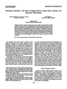
first test case, we consider the unsteady Rayleigh problem [11,12,23] involving a subsonic gas flow at an initially uniform velocity parallel to an infinitely long stationary wall. Here the gas is argon, both gas and wall temperatures are set to 300 K, and a thermal accommodation coefficient (TAC) of 1.0 is used at the wall. The initial gas velocity is 64:5 m=s, corresponding to a Mach number of 0.2, and the number density is set to 1:4 � 1021 m�3 for a mean free path (�) of approximately 0.001 m. An LD simulation is performed on a 0.5 m grid, divided into 50 cells of uniform length with 20 particles per cell and a time step interval of 10�5 s. A symmetry boundary condition is used along the simulation domain boundary opposite the wall, and periodic boundary conditions are used elsewhere to avoid any transverse gradients. For comparison, a DSMC simulation of the same flow is performed on a grid of equal length with 500 cells, 104 particles per cell, and a time step of 10�6 s, such that the cell size and time step are refined to about one mean free path and half the mean collision time, respectively. Both simulations are run for a total elapsed time of 0.01 s, and cell-averaged bulk velocity profiles at the final time step are shown in Fig. 1 for the portion of the simulation domain within 0.25 m of the wall. Note that the DSMC simulation employs a total of 5 � 106 particles and 104 time steps, whereas the LD simulation uses only 1000 particles and 1000 time steps. The DSMC simulation was performed on 16 processors in a large parallel cluster and required approximately 14.4 CPU hours. In contrast, the LD simulation was run in under 2 s on a single processor, which corresponds to an efficiency increase relative to DSMC of over 4 orders of magnitude. Although this scale of efficiency increase may seem surprising, it should be emphasized that DSMC is far more computationally expensive than nearly any continuum simulation method when applied to a near-equilibrium flow, due to stringent DSMC cell size and time step requirements. The efficiency increase for this case is further enhanced by differences in the level of statistical scatter; far more particles per cell are required in a DSMC simulation than in an LD simulation for comparable scatter when no temporal or ensemble averaging is employed. The DSMC and LD velocity profiles in Fig. 1 show excellent overall agreement, although the scatter in DSMC data points is far greater than that observed in the LD results. (If a similar number of particles per cell had been used in the DSMC simulation as in the LD simulation, the scatter in DSMC would likely have been sufficient to make any meaningful comparison of instantaneous velocity profiles impossible.) Both profiles show a smooth boundary layer with a nearly constant slope near the wall and a relatively uniform velocity beyond about 0.15 m from the wall. For comparison, the theoretical solution [23] to the unsteady Rayleigh problem is also included in the plot, with a viscosity calculated from the same VHS model expressions [6] used to evaluate the viscosity in the LD method. Small but noticeable
where uj , �, and T designate the cell bulk velocity, density, and temperature, respectively. For a cell that borders a wall boundary, the total viscous changes in cell momentum and energy are calculated as a summation of Eqs. (4) and (8). Following the evaluation of Eqs. (4) and (8), the quantities �Mi and �E are used to update cell-based velocity and temperature values as given in step 3 of the LD particle method procedures listed earlier. Note that Eqs. (4) and (8) are given for a two-dimensional simulation only. The three-dimensional case would include the addition of extra terms corresponding to the additional tangent vector required to describe an orthonormal coordinate system aligned with each cell face. For example, in a three-dimensional simulation, given a set of orthogonal unit vectors �t1i ; t2i � that are both tangent to a wall boundary face, the quantity �ti tj �f uj in Eqs. (8) will be replaced by �t1i t1j �f uj � �t2i t2j �f uj .
III.
Evaluation of Viscous Flow Modifications
A series of simple one-dimensional test cases are used to independently evaluate diffusive momentum and energy transport in the LD method with modifications for viscous flow simulation. In the
Fig. 1
Velocity profiles for the unsteady Rayleigh flow at 0.01 s.
BURT AND BOYD
1511
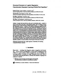
disagreement is shown in boundary-layer profiles between the theoretical solution and both the LD and DSMC velocity profiles. This disagreement can be attributed to the no-slip wall boundary condition used in the theoretical solution, whereas a nonzero velocity is found in cells bordering the wall in the DSMC and LD results. To evaluate the influence of this velocity jump, a second LD simulation is performed with the bulk velocity fixed at zero in the cell bordering the wall. The velocity profile from this additional simulation shows very good agreement with the exact solution, and only a small discrepancy between the two profiles is noticeable in the region of maximum curvature around 0.1 m outward from the wall. To evaluate the effectiveness of the slip model employed in LD calculations, additional LD and DSMC simulations are run with a TAC value of 0.1. A lower accommodation coefficient should make wall slip effects more prominent, so that such effects can be more easily assessed in a comparison of boundary-layer profiles. Results from these additional simulations are shown in Fig. 1. As in the results described earlier for simulations with TAC � 1:0, the two simulations with TAC � 0:1 show excellent overall agreement, with a considerable reduction in statistical scatter for the LD data points. Some small but noticeable difference is found, however, between the wall slip velocities from the two simulations, although much of this difference is likely due to scatter in the DSMC results. A second test case is used to assess diffusive energy transport in the LD method. This is also a one-dimensional unsteady problem and involves an impulsively heated wall bordering an initially quiescent gas of uniform temperature. Here the wall temperature is set to 400 K, the initial gas temperature is 300 K, the wall TAC value is 1.0, and the other physical and numerical parameters are identical to those in the previous case. The only further difference between the LD simulation of this flow and the first LD simulation for the unsteady Rayleigh flow is in the number of particles per cell. Because the pressure should be nearly uniform across the boundary layer where a temperature gradient exists, there must also be a gradient in gas density. As the density is initially constant, a finite bulk velocity will develop in the boundary layer and some LD particles will move between cells. The resulting fluctuations in cell-averaged conserved quantities should produce some scatter in the LD temperature profile. To more clearly compare trends between LD and DSMC simulations, this scatter is reduced by using 100 particles per cell instead of 20 as in the previous case. Temperature profiles from both the LD and DSMC simulations at an elapsed time of 0.01 s are shown in Fig. 2. Very good overall agreement is found between the two results in Fig. 2. In this case, a relatively lower level of scatter is found in the LD temperature profile, although 100 times fewer particles per cell are employed in the LD simulation. Despite the scatter in both results,
the level of agreement found here is a convincing indication that diffusive energy transport is properly handled in the LD method. To more clearly assess the effectiveness of the wall slip boundary condition used in LD calculations, additional LD and DSMC simulations are run with TAC � 0:1. Temperature profiles from these simulations at 0.01 s are shown in Fig. 2. Reasonably good agreement is observed between the LD and DSMC results, with some noticeable difference in the magnitude of temperature jump at the wall. As in the TAC � 1:0 case, differences between the two temperature profiles are dominated by statistical scatter, particularly in the DSMC data points.
Fig. 2 Temperature profiles for flow over an impulsively heated wall at 0.01 s.
Fig. 3 Relative location of buffer regions in a hybrid LD-DSMC simulation.
IV. Hybrid Simulation Procedures Using the Modified Low-Diffusion Method As discussed in the Introduction, the original LD method for inviscid flow simulation has recently been integrated into a hybrid code with DSMC for the simulation of flows involving both continuum and nonequilibrium regions. Hybrid code implementation is relatively straightforward and involves few additional procedures not already present in either the DSMC or LD methods, as described in a previous paper [19]. In the hybrid algorithm, a continuum breakdown parameter based on the density gradient is periodically evaluated in all cells within the computational grid, and breakdown parameter values are compared with a predefined cutoff value to determine whether each cell should be assigned to either DSMC or LD domains. Continuum breakdown is assumed to occur when the condition � � � � > 0:02 (9) max jr�j; � L is satisfied, where � is the local mean free path, � is the gas density, and L is a characteristic global length scale. Two layers of buffer cells, with each layer two cells thick, are employed along the boundary between DSMC and LD domains and are designated as buffer regions A and B. The relative locations of these buffer regions are shown in Fig. 3. In buffer region A, adjacent to the DSMC domain, all simulation procedures are carried out as in DSMC cells, whereas in buffer region B, adjacent to the LD domain, standard LD routines are performed. Just before particle movement procedures during each time step, all particles in both buffer regions are cloned. Newly generated clone particles in region A are given LD-type particle characteristics and are assigned velocity and temperature values based on cell-averaged properties. (To reduce scatter in cell-based property values for cells within buffer region A, these values are averaged over a large number of time steps using a subrelaxation technique as described in [19]). Likewise, newly generated clone particles in region B are given velocity and internal energy values sampled from equilibrium distributions corresponding to cell-averaged properties and are assigned temperature values of zero to designate them as DSMC-type particles. For clarity, it should be noted that, immediately following clone particle generation in
1512
BURT AND BOYD
these buffer regions, all cells in regions A and B should contain an equal number of DSMC- and LD-type particles. Following particle movement procedures, all LD-type particles in buffer region A are removed from the simulation, and all DSMC-type particles in region B are removed as well. This provides a simple and effective means of strongly coupled information transfer between the LD and DSMC domains. Note, however, that mass, momentum, and energy are only conserved during this information transfer in an average sense, and there is some potential for random walk errors. The reader is referred to [19] for further details on hybrid code implementation. For implementation of the LD method with viscous flow modifications in a hybrid LD-DSMC code, few adjustments are required to the procedures already outlined. All procedures are identical other than those related to velocity sampling for DSMCtype clone particles in buffer region B. As found in previous work on hybrid CFD-DSMC simulations employing the Navier–Stokes equations [3,11], significant errors may result when newly generated particles entering a DSMC cell from the CFD domain are assigned velocities from a Maxwellian distribution. These errors are particularly large when strong gradients exist along the interface between the DSMC and CFD domains, as in boundary layers that include both continuum and nonequilibrium regions. To properly account for gradients at the CFD-DSMC interface, particle velocities should be sampled from a Chapman–Enskog distribution instead of a Maxwellian distribution. An efficient acceptance–rejection scheme [24] is therefore used here to generate velocities from a first-order Chapman–Enskog distribution for newly generated DSMC-type clone particles. Note that the Chapman–Enskog distribution includes both velocity and temperature gradients. These gradients are computed in all cells within buffer region B during each time step. The cell-based temperature gradient in a two-dimensional planar simulation may be found through a first-order approximation using the divergence theorem, N
f @T 1 X � A �Tni �f @xi Vc f f
(10)
where Vc is the cell volume, and the temperature at a face is evaluated as an unweighted average of cell-based temperatures for cells on either side of the face. An additional term, �T=r�c , must be subtracted from the right side of Eq. (10) for evaluations of the radial temperature derivative @T=@r in an axisymmetric simulation. Velocity gradients are computed in a similar manner.
V. Hybrid Scheme Evaluation As a representative test case for the evaluation of the LD-DSMC hybrid algorithm with viscous modifications, we consider a flow of N2 through a small convergent–divergent nozzle into a vacuum chamber. This flow was previously used in a study by Boyd et al. [25] in which experimental measurements of pitot pressure along the nozzle exit plane and in the near-field plume region were compared with results from uncoupled CFD and DSMC simulations. In the numerical approach of Boyd et al., a DSMC simulation was run for a flowfield domain beginning slightly downstream of the nozzle throat, and nonuniform DSMC inflow boundary conditions were taken from the results of an independent Navier–Stokes CFD simulation for the nozzle flow. DSMC is required for the accurate simulation of the divergent nozzle and plume regions where nonequilibrium effects are significant, but a DSMC simulation including the high-density convergent nozzle region would have been prohibitively expensive. The uncoupled hybrid approach used in this study therefore provided an effective balance between accuracy and efficiency, and good general agreement was found between the experiment and simulation results. It should be emphasized, however, that the uncoupled CFD-DSMC approach is limited to a narrow range of applications, for which flow along the interface between the two simulation domains is uniformly
supersonic in the direction normal to the interface and unsteady effects can be neglected. Moreover, this approach requires that the continuum breakdown boundary be known before DSMC calculations are performed and involves setup and grid generation for two independent simulations using different sets of input parameters. None of these limitations apply to strongly coupled hybrid schemes such as the LD-DSMC scheme presented here. An axisymmetric hybrid LD-DSMC simulation of this same flow is performed for comparison with published data, using the grid geometry and flowfield parameters given by Boyd et al. [25]. The nozzle has a throat diameter of 3.18 mm, a divergence half-angle of 20 deg, and an area ratio of 100 in the divergent section. The simulation domain extends 4 cm beyond the nozzle exit in the axial direction and 5 cm radially outward from the central axis. The grid boundary geometry is shown in Fig. 4. Gas flow parameters include a stagnation temperature of 699 K, a stagnation pressure of 6400 Pa, a mass flow rate of 6:8 � 10�5 kg=s, and an ambient temperature and pressure of 300 K and 10�2 Pa, respectively, in the vacuum chamber. The nozzle wall is assumed to have a temperature of 587 K and a thermal accommodation coefficient of 1.0. The hybrid simulation is performed using a modified version of the DSMC code MONACO [26], with all DSMC and LD calculation routines fully parallelized for efficient operation on large clusters. The DSMC calculations here employ non-Cartesian subcells with dimensions of roughly one-half the local mean free path, and the VHS model is used along with the no-time-counter scheme of Bird [1] to select DSMC collision pairs during each time step. Translational-rotational energy exchange during simulated DSMC collisions is determined using the Larsen–Borgnakke model [1] along with the model of Boyd [27], in which the inelastic collision probability is evaluated as a function of the total collision energy. As in [19], all cells in the grid are periodically (once every 500 time steps) assigned to DSMC, LD, or buffer regions. During this assignment procedure, continuum breakdown is evaluated in each cell using Eq. (9), with the characteristic global length scale L set to equal the nozzle throat diameter. Numerical weight factors (the number of real molecules represented by each particle in the simulation) are assigned to each cell roughly in proportion to cell volume, and several bands of constant numerical weight are used to reduce random walk errors associated with cloning and removal procedures when particles move between cells with different weight values. Although most cells in the divergent nozzle region and all cells in the plume can be assigned to the same constant-weight band, large differences in weight values are required in regions upstream of the throat to avoid excessive particle populations in some cells while assuring that each cell, on average, contains at least 20 particles. A structured grid with 38,200 quadrilateral cells is used in the hybrid simulation. All cells in regions of expected continuum breakdown are refined to less than two local mean free paths, and cells in continuum regions are sufficiently refined to assure grid independence. (Grid independence was confirmed by running an additional simulation with much smaller cells in high-gradient regions and assuring that any differences in various flow quantities are no larger than a few percent.) The simulation employs a uniform global time step interval of 10�8 s. This interval was estimated to meet DSMC time step requirements in cells expected to be within the
Fig. 4 Grid geometry, LD and DSMC domains, and streamlines in the hybrid nozzle/plume flow simulation.
1513
BURT AND BOYD
DSMC domain and to meet a less restrictive Courant–Friedrichs– Lewy criterion [28] in other cells within the probable LD domain. The flowfield is initialized at simulation startup with subsonic nozzle inflow conditions upstream of the throat and with vacuum chamber ambient conditions elsewhere. Calculations are performed for a startup period of 100,000 time steps, followed by a sampling period of another 100,000 time steps after convergence to steady state. The simulation requires about 30 h on 20 AMD Opteron processors in the NYX cluster at the University of Michigan. As an additional source of data for comparison with LD-DSMC simulation results, a set of CFD and DSMC simulations for this flow is performed using the same uncoupled procedure as the simulations of Boyd et al. [25]. A CFD simulation is run for the flow within the nozzle, and a DSMC simulation is then run for the divergent nozzle region and plume. Flow properties along the nonuniform DSMC inflow boundary, which is located approximately 1 mm downstream of the nozzle throat, are extracted from CFD results at the inflow boundary location. The DSMC simulation is performed with the same code [26] that is used as a basis for the hybrid LD-DSMC code, and the same DSMC models are used in the DSMC simulation as in the hybrid LD-DSMC simulation. Thus, a comparison of LD-DSMC results and results from the uncoupled DSMC simulation should allow for an assessment of hybrid scheme accuracy independent of any DSMC modeling approximations. The CFD nozzle flow simulation is performed using the LeMANS code [20] developed at the University of Michigan. A second-order point implicit simulation is run using a finite volume discretization of the axisymmetric compressible Navier–Stokes equations, and a modified low-dissipation version of Steger–Warming flux vector splitting is used to evaluate fluxes along cell faces. As in the LD particle method, no consideration is made for rotational nonequilibrium effects, and vibrational excitation is neglected due to the low temperature range in this flow. Although the LeMANS code was developed for the simulation of hypersonic blunt body flows, a recent unpublished study has shown very good overall accuracy when LeMANS calculations are applied to the flow regimes experienced in this nozzle flow case. However, assumptions used in LeMANS that the flow is supersonic along inflow boundaries result in an increase in mass flow of about 3.5% relative to the desired value of 6:8 � 10�5 kg=s, as measured by Boyd et al. [25]. For a better comparison of results from the hybrid LD-DSMC simulation and the uncoupled CFD and DSMC simulations, the inflow number density in the hybrid simulation is adjusted to match this increased mass flow rate. Streamlines and domain boundaries at steady state in the hybrid LD-DSMC simulation are shown in Fig. 4. The LD domain includes high-density near-equilibrium regions upstream and some distance downstream of the nozzle throat, whereas the DSMC domain comprises remaining portions of the divergent nozzle region and plume. Streamlines show generally expected trends, with smooth convergence toward the throat and a gradual increase in divergence angles downstream of the nozzle exit plane. The contours of a density-based gradient length local Knudsen number [29] from the LD-DSMC simulation are shown in Fig. 5. This is the same nondimensional parameter used in Eq. (9) as part of the continuum breakdown criterion for the assignment of cells to LD or DSMC domains; it can be viewed as one indicator of the local validity of near-equilibrium assumptions underlying the Navier– Stokes equations. These same assumptions (in particular, that the velocity distribution is a small perturbation from a Maxwellian distribution) are used as a basis for the LD method and are thought to be valid so long as the ratio of the mean free path to characteristic gradient length scales is much less than 1. From the contour lines in Fig. 5, it follows that such near-equilibrium assumptions become progressively less suitable with increasing distance from the central axis in the divergent nozzle and plume regions. As expected, a very high degree of nonequilibrium is observed around the nozzle lip, due to considerable density gradients and large mean free path values associated with a strong centered expansion in this region. Figure 6 shows contours of density from the hybrid simulation, with values normalized by the stagnation density. The figure shows a
Fig. 5 Contours of the gradient length local Knudsen number based on density.
density reduction of over 5 orders of magnitude between the stagnation region upstream of the nozzle and the far-field plume region near the nozzle exit plane. There is a particularly large density range in the region of rapid expansion around the nozzle lip, and a small density increase near the wall in the convergent nozzle region corresponding to a temperature reduction in the boundary layer along the relatively cool isothermal wall. Contours of Mach number are shown in Fig. 7. As in Fig. 6, the Mach number contour plot shows an area near the axis in the divergent nozzle region where radial gradients are small and where the flow may be roughly characterized as a quasi-one-dimensional isentropic expansion. Further from the axis, large radial gradients appear as a result of the increased streamline divergence angles and the presence of a thick boundary layer along the nozzle wall. As expected, sonic lines are observed in Fig. 7 at the throat and within the boundary layer in the convergent nozzle region, with a sonic point at the nozzle lip. An additional subsonic region is found far from the axis near the nozzle exit plane and is thought to appear as a result of the finite ambient density in the simulated vacuum chamber. In Figs. 8–10, results from the hybrid LD-DSMC simulation along a radial plane a small distance (0.6 mm) downstream of the nozzle throat are compared with results from CFD Navier–Stokes simulations. Curves labeled CFD (1) are taken from the LeMANS [20] nozzle flow simulation performed as part of this study, whereas curves labeled CFD (2) are from the CFD simulation of Boyd et al.
Fig. 6
Contours of density from the hybrid LD-DSMC simulation.
Fig. 7
Mach number contours.
1514
Fig. 8
BURT AND BOYD
Profiles of bulk velocity magnitude near the nozzle throat.
[25]. Although CFD results should ideally be independent of the scheme employed in the CFD calculations, it should be noted that the simulation of Boyd et al. involves a very different set of numerical techniques than LeMANS. This simulation was performed using the second-order explicit two-step MacCormack method, with additional likely differences from LeMANS in physical modeling assumptions such as the temperature dependence of transport coefficients. Differences in algorithms and physical models between the two CFD simulations may account for any disagreement observed in the CFD results, although insufficient information is presented by Boyd et al. [25] to allow any definite explanations for such disagreement. Figure 8 shows profiles of bulk velocity magnitude from the hybrid LD-DSMC simulation and both CFD simulations. Velocity values are normalized by the most probable thermal speed at the stagnation conditions, and radial coordinates are normalized by the nozzle throat diameter. We find excellent overall agreement between all three curves of Fig. 8, with particularly good agreement between the LD-DSMC and CFD (1) results. The maximum difference in throat velocity profiles is near the “shoulder” in the profile at the outer edge of the boundary layer, where the CFD (2) value is about 3% higher than the values from the other two simulations. Although no clear explanation for this difference can be found, the high level of agreement in this region between the other two simulation results indicates that the difference is not likely a result of fundamental problems in the LD particle method or its implementation in the hybrid scheme. Note that a nonzero velocity is found along the wall in the hybrid simulation as a result of the slip model employed in the LD method procedures. Although no-slip model is used in either CFD simulation, the magnitude of velocity slip here can be assumed accurate based on the comparison with DSMC boundary-layer profiles in Sec. III. Although the presence of a nonzero slip velocity has a minimal impact on the hybrid velocity profile in Fig. 8, we expect this slip effect to significantly influence surface properties such as wall shear stress. Figure 9 shows profiles of temperature, normalized by the stagnation temperature, slightly downstream of the throat in the hybrid simulation and the LeMANS CFD simulation. (No corresponding temperature data were provided for the CFD simulation of Boyd et al., and so results from this additional CFD simulation cannot be used here for comparison.) Overall agreement here is excellent, with differences at the central axis of around 0.1%. Noticeable disagreement is found, however, in an area some distance away from both the axis and the wall, where a slight underprediction in temperature is observed in the hybrid results. The maximum local temperature difference here is about 2.6%, and occurs at a normalized radial coordinate of around 0.4. Normalized density profiles near the throat are shown in Fig. 10. As with temperature data, no information for gas density near the
Fig. 9
Temperature profiles near the nozzle throat.
Fig. 10
Density profiles near the nozzle throat.
throat is available for the CFD simulation of Boyd et al., and so only the LeMANS CFD simulation is used for comparison with the hybrid simulation results. As in Fig. 9, excellent overall agreement is observed in throat density profiles between the two simulations. The maximum difference occurs at the central axis, where density is underpredicted in the hybrid simulation by about 2.7%. Figure 11 shows profiles of bulk velocity magnitude at the nozzle exit from the hybrid LD-DSMC simulation and from uncoupled sets of CFD and DSMC simulations as described earlier. The curve labeled CFD/DSMC (1) is taken from results of the uncoupled MONACO [26] DSMC simulation performed as part of the present study, whereas the curve labeled CFD/DSMC (2) is from the published data of Boyd et al. [25]. Velocity values in Fig. 11 are normalized by the characteristic thermal speed for N2 at the stagnation temperature, and radial coordinates are normalized by the nozzle exit diameter. As in the throat velocity profiles shown in Fig. 8, remarkably good agreement is found between the hybrid simulation results and results from additional simulations performed for comparison as part of the present study. The maximum local difference between the hybrid and CFD/DSMC (1) exit plane velocity profiles is about 0.1%. In contrast, significant differences exist between the velocity profile of Boyd et al. and the other two curves. No clear explanation for these differences is apparent, although the level of agreement between hybrid simulation and CFD/ DSMC (1) results makes any large differences caused by errors in the hybrid algorithm seem unlikely.
1515
BURT AND BOYD
Fig. 11
Velocity profiles at the nozzle exit.
The profiles of translational and rotational temperature along the nozzle exit plane are shown in Fig. 12. Temperature values are normalized by the stagnation temperature. Note that the throat temperature profiles in Fig. 9 are taken within the LD domain for the hybrid LD-DSMC simulation, where there is no distinction between translational and rotational temperatures. These temperatures may be considered independently at the nozzle exit in the hybrid simulation, because this region is well within the DSMC domain shown in Fig. 4. In Fig. 12, very good agreement is found between results from all three simulations; both translational and rotational temperature profiles from the hybrid simulation and MONACO DSMC simulation are nearly indistinguishable. Significant rotational temperature lag is observed in all results within an area some distance from the central axis. This trend may be attributed in part to the low collision frequency, large rotational collision number, and streamwise translational temperature gradients associated with a rapid expansion in this region. Normalized density profiles along the nozzle exit from the hybrid LD-DSMC simulation and the uncoupled MONACO DSMC simulation are shown in Fig. 13. (No corresponding data from the DSMC simulation of Boyd et al. are available for comparison.) As with other results from these two simulations, the overall level of agreement is excellent. The largest local difference between density values at the nozzle exit is approximately 1.7%, and occurs at a normalized radial coordinate of about 0.1.
Fig. 12 Temperature profiles at the nozzle exit.
Fig. 13 Density profiles at the nozzle exit.
In Fig. 14, pitot pressure profiles at the nozzle exit are compared between results from the hybrid LD-DSMC simulation, the two uncoupled sets of CFD and DSMC simulations, and the experimental measurements of Boyd et al. [25]. The pitot pressure is determined from numerical data by calculating the local stagnation pressure behind a shock, using normal shock relations for pressure and Mach number along with the isentropic relation between the static and stagnation pressures [30]. A correction to the stagnation pressure for rarefaction effects is employed, as described by Boyd et al. [25], and resulting values are normalized in Fig. 14 by the stagnation pressure at the nozzle entrance. Note that these pitot pressure values are functions of velocity, temperature, and density, and so the extremely good agreement found in Fig. 14 between the hybrid and CFD/ DSMC (1) profiles is expected due to the similar levels of agreement observed for these simulations in Figs. 11–13. Reasonably good agreement is also found between the hybrid results and the experimental and numerical data of Boyd et al. However, all numerical results significantly underpredict pitot pressure in the low-density region near the nozzle lip. Because of the consistency of all numerical data in this region, one likely explanation for the large differences between the experiment and simulation results is inaccuracy associated with the rarefaction correction [25] for numerical pitot pressure values. This correction is inherently approximate and provides only a simple phenomenological estimation of a series of complex nonequilibrium effects. Additional differences are found near the central axis, where the uncoupled
Fig. 14
Profiles of pitot pressure at the nozzle exit.
1516
BURT AND BOYD
DSMC simulation results of Boyd et al. agree considerably better than either the hybrid or CFD/DSMC (1) results with the experimental values. Despite these differences, the good overall level of agreement between the hybrid LD-DSMC simulation results and experimental data can be seen as an indication that the hybrid scheme is sufficiently effective and accurate as applied to this test case. In contrast to the uncoupled CFD/DSMC approach used here for comparison, the hybrid scheme allows the entire flowfield of interest to be included in a single simulation and avoids the various restrictions that tend to limit such an uncoupled approach to a narrow class of steady-state supersonic flow problems.
VI.
Conclusions
A DSMC-based LD particle method for compressible inviscid gas flow simulation has been extended for use with near-equilibrium viscous flows involving a simple gas. A finite volume discretization of viscous terms in the compressible Navier–Stokes equations has been integrated into LD particle method procedures, so that the method may be applied to low-Knudsen-number flows that include boundary layers, free shear layers, or other phenomena for which viscous effects are important. With these viscous flow modifications, the LD method should be applicable to the same Knudsen number range as the Navier–Stokes equations. A wall slip model has also been implemented to improve accuracy for simulations in the slip flow Knudsen number regime. Results from a series of unsteady boundary-layer simulations using the modified LD particle method were compared with corresponding DSMC results and a theoretical solution. Overall excellent agreement was found, with a much lower level of statistical scatter in the LD data points than in the DSMC data. For these flow problems, the computational expense of LD simulations was found to be roughly 4 orders of magnitude lower than that of DSMC simulations, due to reduced scatter as well as the far less restrictive cell size and time step requirements for the LD method. Although such a large efficiency increase relative to DSMC may seem very encouraging, it should be emphasized that nearly any scheme intended for continuum flow simulation will be orders of magnitude more efficient than DSMC when applied to sufficiently high-density conditions. In a previous study [18] involving simulations of an inviscid flow with complex shock interactions, the LD method was estimated to be approximately 20–50 times more efficient than other DSMC-based continuum flow simulation methods and around 16 times more efficient than a CFD simulation using the LeMANS code [20]. The LeMANS simulation involved an implicit second-order discretization of the Euler equations, using a modified form of Steger– Warming flux vector splitting. As the LeMANS code is optimized for very different conditions than those of the test case used in this comparison, it is likely that other compressible CFD codes would show considerable efficiency improvements for this case relative to LeMANS. We expect that a modern high-order implicit CFD algorithm will be far more efficient than the LD particle method. However, as described in the Introduction, the implementation of such an algorithm in a hybrid code with DSMC presents enormous difficulties and physical limitations. Furthermore, in a wide range of potential applications for this type of hybrid code, a large fraction of the flowfield must be assigned to DSMC and the total simulation cost is only weakly dependent on the efficiency of the continuum method. Procedures have been outlined for the integration of the LD particle method with viscous modifications into a strongly coupled hybrid algorithm with DSMC for the efficient simulation of flows involving nearly any combination of Knudsen number regimes. Although implementation of such a hybrid scheme is inherently complex, the relatively small number of required alterations and additions to the base DSMC code likely make this the simplest proposed extension of DSMC to near-equilibrium viscous flows, which allows for the proper resolution of high-gradient regions even when the cell size and time step are far larger than the mean free path and mean collision time, respectively. In contrast to coupled CFDDSMC algorithms intended for the simulation of similar flows, the
continuum component of the hybrid code is built around standard DSMC procedures, so that no integration of separate source codes is required, and all LD and hybrid simulation routines in the LD-DSMC algorithm constitute an addition to the DSMC source code length of no more than about 20%. In contrast, a coupled CFD-DSMC algorithm may require an addition of more than 100% to the DSMC source code, including both a continuum CFD solver and routines for domain decomposition and communication between CFD and DSMC components [6]. A flow of N2 through a small convergent–divergent nozzle into a vacuum chamber was chosen as a test case to evaluate the hybrid LDDSMC scheme. Various flow properties were compared between results from an LD-DSMC simulation and results from a series of uncoupled CFD and DSMC simulations. Available experimental data for pitot pressure at the nozzle exit were also used for comparison. Very good overall agreement was found between the LDDSMC simulation results and other numerical and experimental data, with particularly good agreement between hybrid data points and values from the CFD and DSMC simulations performed as part of the present study. Although these comparisons should not be viewed as a rigorous validation of the proposed hybrid scheme, the lack of any large differences between the hybrid simulation results and those from other simulations is an encouraging indication of overall accuracy and suitability for general application to rarefied expansion flows. Although the current implementation of the hybrid LD-DSMC scheme allows for the relatively efficient simulation of a wide range of flows, including steady or unsteady laminar flows that involve nearly any combination of Knudsen number regimes for a simple dilute gas, a number of planned modifications to this scheme may further extend the range of possible applications. One important limitation of the current scheme is the simple gas assumption used in viscous modifications to the LD method, which makes this method incompatible with flow problems involving a gas mixture. Viscous phenomena associated with mixtures include mass diffusion, additional dissipative terms in the gas energy balance, and a potentially complex dependence of transport coefficients on species concentrations. Future improvements to the LD-DSMC scheme will involve consideration of such phenomena through the inclusion of species diffusion velocities in the motion of Lagrangian faces within the LD domain and the use of mixing rules for transport coefficients based on kinetic theory approximations. Additional proposed extensions to the LD method include modifications for rotational and vibrational nonequilibrium using models analogous to those employed in DSMC and implementation of DSMC-type chemistry models for reacting flow simulations.
Acknowledgments Partial financial support for this work was provided by NASA through grant NNX08AD02A. Additional support was provided by Spectral Sciences, Inc., through contract W9113M-06-C-0122, a Missile Defense Agency Small Business Innovative Research Phase II award. The authors gratefully acknowledge Jason Cline and Matt Braunstein for their oversight of this work. The authors would also like to thank Matt McKeown at the University of Michigan for his help with the CFD simulations that were performed as part of this study.
References [1] Bird, G. A., Molecular Gas Dynamics and the Direct Simulation of Gas Flows, Clarendon Press, Oxford, 1994. [2] Hueser, J. E., Melfi, L. T., Bird, G. A., and Brock, F. J., “Analysis of Large Solid Propellant Rocket Engine Exhaust Plumes Using the Direct Simulation Monte Carlo Method,” AIAA Paper 84-0496, 1984. [3] Hash, D. B., and Hassan, H. A., “A Decoupled DSMC/Navier–Stokes Analysis of a Transitional Flow Experiment,” AIAA Paper 96-0353, 1996. [4] VanGilder, D. B., Chartrand, C. C., Papp, J., Wilmoth, R., and Sinha, N., “Computational Modeling of Nearfield to Farfield Plume Expansion,” AIAA Paper 2007-5704, 2007.
BURT AND BOYD
[5] Schwartzentruber, T. E., and Boyd, I. D., “A Hybrid ParticleContinuum Method Applied to Shock Waves,” Journal of Computational Physics, Vol. 215, 2006, pp. 402–416. doi:10.1016/j.jcp.2005.10.023 [6] Schwartzentruber, T. E., and Boyd, I. D., “A Modular ParticleContinuum Numerical Method for Hypersonic Non-Equilibrium Gas Flows,” Journal of Computational Physics, Vol. 225, 2007, pp. 1159– 1174. doi:10.1016/j.jcp.2007.01.022 [7] Lian, Y.-Y., Wu, J.-S., Cheng, G., and Koomullil, R., “Development of a Parallel Hybrid Method for the DSMC and NS Solver,” AIAA Paper 2005-0435, 2005. [8] Roveda, R., Goldstein, D. B., and Varghese, P. L., “Hybrid Euler/ Particle Approach for Continuum/Rarefied Flows,” Journal of Spacecraft and Rockets, Vol. 35, No. 3, 1998, pp. 258–265. doi:10.2514/2.3349 [9] Roveda, R., Goldstein, D. B., and Varghese, P. L., “Hybrid Euler/Direct Simulation Monte Carlo Calculation of Unsteady Slit Flow,” Journal of Spacecraft and Rockets, Vol. 37, No. 6, 2000, pp. 753–760. doi:10.2514/2.3647 [10] Wadsworth, D. C., and Erwin, D. A., “Two-Dimensional Hybrid Continuum/Particle Approach for Rarefied Flows,” AIAA Paper 922975, 1992. [11] Garcia, A. L., Bell, J. B., Crutchfield, W. Y., and Alder, B. J., “Adaptive Mesh and Algorithm Refinement Using Direct Simulation Monte Carlo,” Journal of Computational Physics, Vol. 154, 1999, pp. 134–155. doi:10.1006/jcph.1999.6305 [12] Breuer, K. S., Piekos, E. S., and Gonzales, D. A., “DSMC Simulations of Continuum Flows,” AIAA Paper 95-2088, 1995. [13] Titov, E. V., Zeifman, M. I., and Levin, D. A., “Application of the Kinetic and Continuum Techniques to the Multi-Scale Flows in MEMS Devices,” AIAA Paper 2005-1399, 2005. [14] Pullin, D. I., “Direct Simulation Methods for Compressible Inviscid Ideal-Gas Flow,” Journal of Computational Physics, Vol. 34, 1980, pp. 231–244. doi:10.1016/0021-9991(80)90107-2 [15] Macrossan, M. N., “A Particle-Only Hybrid Method for NearContinuum Flows,” Rarefied Gas Dynamics: 22nd International Symposium, American Institute of Physics, College Park, MD, 2001, pp. 388–395. [16] Tiwari, S., and Klar, A., “An Adaptive Domain Decomposition Procedure for Boltzmann and Euler Equations,” Journal of Computational and Applied Mathematics, Vol. 90, 1998, pp. 223–237. doi:10.1016/S0377-0427(98)00027-2 [17] Macrossan, M. N., “The Equilibrium Flux Method for the Calculation of Flows with Non-Equilibrium Chemical Reactions,” Journal of
[18]
[19]
[20] [21] [22]
[23] [24]
[25]
[26]
[27]
[28] [29] [30]
1517 Computational Physics, Vol. 80, 1989, pp. 204–231. doi:10.1016/0021-9991(89)90095-8 Burt, J. M., and Boyd, I. D., “A Low Diffusion Particle Method for Simulating Compressible Inviscid Flows,” Journal of Computational Physics, Vol. 227, 2008, pp. 4653–4670. doi:10.1016/j.jcp.2008.01.020 Burt, J. M., and Boyd, I. D., “A Hybrid Particle Approach for Continuum and Rarefied Flow Simulation,” Journal of Computational Physics, Vol. 228, 2009, pp. 460–475. doi:10.1016/j.jcp.2008.09.022 Scalabrin, L. C., and Boyd, I. D., “Development of an Unstructured Navier–Stokes Solver for Hypersonic Nonequilibrium Aerothermodynamics,” AIAA Paper 2005-5203, 2005. Vincenti, W. G., and Kruger, C. H., Introduction to Physical Gas Dynamics, Krieger, Malabar, FL, 1986. Chou, S. Y., and Baganoff, D., “Kinetic Flux-Vector Splitting for the Navier–Stokes Equations,” Journal of Computational Physics, Vol. 130, 1997, pp. 217–230. doi:10.1006/jcph.1996.5579 White, F. M., Viscous Fluid Flow, McGraw–Hill, New York, 1991. Garcia, A. L., and Alder, B. J., “Generation of the Chapman–Enskog Distribution,” Journal of Computational Physics, Vol. 140, 1998, pp. 66–70. doi:10.1006/jcph.1998.5889 Boyd, I. D., Penko, P. F., Meissner, D. L., and DeWitt, K. J., “Experimental and Numerical Investigations of Low-Density Nozzle and Plume Flows of Nitrogen,” AIAA Journal, Vol. 30, No. 10, 1992, pp. 2453–2461. doi:10.2514/3.11247 Dietrich, S., and Boyd, I. D., “Scalar and Parallel Optimized Implementation of the Direct Simulation Monte Carlo Method,” Journal of Computational Physics, Vol. 126, 1996, pp. 328–342. doi:10.1006/jcph.1996.0141 Boyd, I. D., “Analysis of Rotational Nonequilibrium in Standing Shock Waves of Nitrogen,” AIAA Journal, Vol. 28, No. 11, 1990, pp. 1997– 1999. doi:10.2514/3.10511 Laney, C. B., Computational Gasdynamics, Cambridge Univ. Press, 1998. Wang, W., and Boyd, I. D., “Hybrid DSMC-CFD Simulations of Hypersonic Flow Over Sharp and Blunted Bodies,” AIAA Paper 20033644, 2003. Anderson, J. D., Modern Compressible Flow with Historical Perspective, McGraw–Hill, New York, 1990.
C. Kaplan Associate Editor