James D. Klett. PAR Associates, 1741 Pomona Drive, Las Cruces, New. Mexico 88001. Received 2 January 1985. 0003-6935/86/152462-03$02.00/0.
Extinction boundary value algorithms for lidar inversion James D. Klett PAR Associates, 1741 Pomona Drive, Las Cruces, New Mexico 88001. Received 2 January 1985. 0003-6935/86/152462-03$02.00/0. © 1986 Optical Society of America. The familiar solution to the single-scattering lidar equa tion predicts extinction as a function of range in terms of (1) the relative signal strength and (2) a reference or boundary value of extinction that is present as an independent con stant of integration. For cases of low visibility the solution is only weakly dependent on this latter parameter, but it can become of critical importance for some circumstances of moderate to high visibility. Algorithms to estimate the extinction boundary value by making use of knowledge of the absolute power level of the return signal are available in the literature.1"3 This Letter presents an alternative set which has been selected on the grounds of simplicity and performance in numerical experi ments. The result is a combination of three models, one valid for cases of low optical depth, another suitable for most cases of moderate to large optical depth, and a third provided largely as a default procedure for somewhat anomalous situa tions that cannot be handled by either of the two principal algorithms. On making the usual assumption that the atmospheric backscatter and extinction coefficients, β and σ, are related according to a power law of the form where B depends on wavelength and various properties of the obscuring aerosol and k ≈ 1, the single-scattering lidar equa tion may be expressed in the form
In this equation P(r) is the instantaneous power received from range r, and the system constant C is given by where P 0 is the transmitted power, c is the velocity of light, r is the pulse duration, and A is the effective system receiver area. For constant k the stable solution to Eq. (2) is
where Sm = S(rm), σm = σ(rm), and r ≤ rm.4 Note that the solution depends on both the relative signal, S - Sm, and the extinction boundary value σm; the latter makes its appear ance as an independent constant of integration, as described above. From Eq. (2) one can attempt to relate σm to the signal strength returned from the maximum useful range rm: 2462
APPLIED OPTICS / Vol. 25, No. 15 / 1 August 1986
However, the contribution of the integral attenuation term over the interval (0,r0), where r0 is the point of transmitter and receiver beam overlap, is unfortunately unknown. Two previously made assumptions about this unknown attenua tion term are that (1) the extinction is constant over the interval (0,r0)2 and (2) the average extinction over (0,rm) is the same as that over (r0,rm)1. On the other hand, the contribution to the attenuation term over the interval (r0,rm) is easily expressed as a function of σm by integration of Eq. (4):
In this last expression the extinction boundary value and the signal integral have been expressed in dimensionless form:
Note that Eq. (9) provides a measure of optical depth over the interval (r0,rm). If we now impose the second of the assumptions described above concerning the attenuation to the crossover point, namely, that
one arrives at the following equation for Ωm1:
where the constant Gm is given by Thus the desired Ωm is located at the intersections of the curve y1 = Gm with the curve (see Fig. 1)
However, it can be seen from the figure that there are no roots if Gm is greater than the maximum of Eq. (11) occurring at Computational experience with the algorithm also shows it to be unreliable for some cases of low visibility. This might be expected from Fig. 1, since the intersection of the two curves for large Ωm occurs where they are nearly parallel; hence a small error in the estimated value of the system constant, for example, might produce a very large error in the root. Because of these difficulties (the possibility of there being no solution if the computed value of Gm is sufficiently in error and the possible error amplification in cases of large optical depth), it has been found useful to employ instead three separate estimation procedures, with each taylored for a range of parameters or set of conditions. For low visibilities, we note from Eq. (7) that the average value of extinction depends primarily on the relatively large magnitude of the
signal integral I, so that an additional constraint is needed to select a unique boundary value of extinction. This suggests the simple approach of determining the boundary value in such cases by setting it equal to the average extinction. Then directly from Eq. (7) one obtains Ωm as the solution to It is easy to show that this equation always has a solution for I > 1 and that it may be obtained in a few iterations starting with an initial small value for Ωm. Any error in the estimate supplied by Eq. (14) will make little difference in the calcu lated visibility for the circumstances for which this particu lar algorithm is intended. For high visibilities the choice of σm influences σ(r) more strongly, there being insufficient optical depth for the wellknown self-convergence property of Eq. (4) to play a signifi cant role. Also, as can be seen from the large intersection angle of the curves in Fig. 1 for the case of the small root, errors in Gm will not be reflected as greatly amplified errors in the root. Hence an alternative to Eq. (14) is appropriate for high visibilities. Although Eq. (11) is suitable for this purpose, a slightly simpler algorithm may be obtained from Eq. (5) by using the previously mentioned alternative as sumption of constant extinction from the lidar to the cross over point. Then Eq. (5) may be expressed in the form This equation may now be solved for the desired extinction boundary value (in dimensionless form): This algorithm is very similar to Mulders's3 modification of the formulation of Ferguson and Stephens.2 In general σ0 is not known unless σm is, but in practice this minor difficulty can be overcome through simple iteration of Eq. (16). For example, one may initially set σ0 = 0 and solve for σm; then from Eq. (4) evaluated at r0 a new value of σ0 is obtained, which may be substituted back into Eq. (16) and so forth. This procedure is successful in the presence of errors because of the stability of Eq. (4). As an example of a case not solvable by either the high or low visibility algorithms, consider an extinction distribution for which I < 1. Ordinarily, this would be interpreted as a typical low optical depth or high visibility situation, and so Eq. (16) would be applied. But if the system constant C is significantly in error, a realistic possibility, it may happen that exp(-G'm) < J, so that Eq. (16) fails completely. One would, therefore, consider turning to Eq. (14), but this option also would fail since for I < 1, Eq. (14) has no solution except Ωm = 0. The failure of Eq. (16) to provide a solution corre sponds graphically to having the line y1 = Ωm situated higher
Fig. 1. Plot of y1 = Gm and y2, given by the right-hand side of Eq. (11), showing the location of the boundary values at the intersections of the curves. 1 August 1986 / Vol. 25, No. 15 / APPLIED OPTICS
2463
Fig. 2. Constant input distribution and the inversion solution hav ing an unrealistic drop-off with range. Both profiles can be used to generate the same calibrated signal. than the maximum in the curve y2. This suggests a simple default strategy to resolve the impasse: make the estimate
in case the high and low visibility algorithms have no solu tions. The ability of the above algorithms to estimate extinction boundary values from input calibrated signals has been test ed numerically using several extinction distributions and assumed errors in the system constant C. From these simu lations, selection rules for the various algorithms have been obtained. They may be summarized as follows: The inver sion of a lidar signal begins by trying the high-visibility algorithm first. It is considered successful if exp(-G m ' ) > I + 0.01 [see Eq. (16)] and if the resulting σm > 0.01 and σ0/σm < 50. Otherwise, a switch to the low-visibility algorithm [Eq. (14)] is made, unless I < 1, in which case the default algorithm [Eq. (17)] is used. From the discussion so far the above selection rules should seem reasonable, except perhaps for the criterion that Eq. (16) is to be rejected if σm < 0.01 or σ 0 /σ m > 50. These slightly arbitrary conditions have come about somewhat par adoxically from trying to apply Eq. (16) to cases of high extinction and are a consequence of the fact that in such cases there are two possible roots to Eq. (16), one very small and easily computed, and the other large and computational ly unreliable due to instabilities of the kind already dis cussed. Probably the easiest way to appreciate the problem of double-valuedness is to consider the lidar signal at the cross over point r 0 . At that location and if the assumption of constant extinction on the interval (0,r0) is assumed, the signal S can be seen from Eq. (2) to have the following form:
Therefore, σ0 is given by the intersection of the curve ƒ1 = (S 0 - C)/k = constant with the curve f2(x) = lnx - x/xc, where xc = k/2r0 is the location of the maximum ofƒ2. The situation is entirely analogous to that illustrated in Fig. 1; and, in partic ular, there are two roots for σ0∙ Consequently, Eq. (16) may converge to a σm corresponding to the physically unreason able very small root to Eq. (18). This in fact will happen for large optical depths, because the high-visibility algorithm is iterated starting with σ0 = 0, as described earlier. The outcome can then be used as an indicator that the highvisibility algorithm is inappropriate for the particular signal being analyzed and should be rejected in favor of the lowvisibility algorithm. 2464
APPLIED OPTICS / Vol. 25, No. 15 / 1 August 1986
As a simple example of this behavior, consider the case of a cosntant extinction distribution of magnitude 9.78/km. For k = C = 1 and with r0 = 15 range point units, the signal value computed from Eq. (18) for this distribution is S0 = 1.227, so that ƒ2(x) = lnx - x/4.76 = 0.227. This equation has the two roots σ01 = 1.85 and σ02 = 9.78. The high-visibility algorithm converges to a boundary value corresponding to the smaller root. The boundary value obtained in this fashion is ex tremely small: σm = 8.8 × 10 - 6 /km. The resulting inversion extinction profile assuming no errors in k or C is shown in Fig. 2. It should perhaps be emphasized that this profile repro duces the input signal just as well as the desired alternative constant distribution σ = 9.78/km, and so can only be reject ed on the basis that it is physically implausible. Numerical experiments with a wide range of extinction distributions, and including errors in the calibration infor mation, show that the overall extinction boundary value algorithm obtained through use of the selection rules is capa ble of providing better results than previously reported indi vidual estimation schemes. Part of this research was performed under contract to the U.S. Army Atmospheric Science Laboratory, White Sands Missile Range, NM 88002. References 1. J. D. Klett, "Lidar Calibration and Extinction Coefficients," Appl. Opt. 22, 514 (1983). 2. J. A. Ferguson and D. H. Stephens, "Algorithm for Inverting Lidar Returns," Appl. Opt. 22, 3673 (1983). 3. J. A. Mulders, "Algorithm for Inverting Lidar Returns: Com ment," Appl. Opt. 23, 2855 (1984). 4. J. D. Klett, "Stable Analytical Inversion Solution for Processing Lidar Returns," Appl. Opt. 20, 211 (1981). 5. J. D. Klett, "Estimation of Extinction Boundary Values for Lidar Inversion," ERADCOM Report ASL-CR-85-0093-1, U.S. Army Atmospheric Sciences Laboratory, White Sands Missile Range, White Sands, NM 88002 (1985), 45 pp.