Extracting Dense Communities from Telecom Call Graphs (Invited Paper) Vinayaka Pandit Natwar Modani Sougata Mukherjea Amit A. Nanavati Sambuddha Roy
Amit Agarwal Department of Statistics and Operations Research University of North Carolina Chapel Hill, North Carolina Email:
[email protected]
IBM India Research Laboratory New Delhi, India Email:
[email protected]
Abstract—Social networks refer to structures made of nodes that represent people or other entities embedded in a social context, and whose edges represent interaction between entities. Typical examples of social networks are collaboration networks in a research community, networks arising out of interaction between colleagues of large organization etc. Social networks are highly dynamic objects that evolve quickly over time with addition and deletion of nodes and edges. Understanding the evolution of a social network is helpful in inferring trends and patterns of social contacts in a particular social context. In this paper, we consider social networks that are derived from Telephone Call Records, i.e, graphs in which the individual phone numbers (and hence its users) are the nodes and the edges correspond to a telephonic contact between the two nodes they connect. We study the problem of extracting dense communities from such Telecom Call Graphs. The problem studied here is set in the context of a larger project. We motivate the problem studied by describing the context in which it is set. Our analysis is based on suitable algorithmic engineering of an approximation algorithm for the densest subgraph problem by Charikar [9]. We present empirical results on massive graphs with millions of nodes and edges. We also discuss many open problems that are important in the context of analyzing telecom call graphs.
I. I NTRODUCTION Social network analysis from the point of view of analyzing telephone calls between people is the focus of this paper. A network (also called as “graph”) consists of a set of vertices (also called as nodes) and a set of edges connecting the vertices. A social network is a network in which the vertices represent entities (or people) set in a social context and edges which indicate evidence of social interaction between the entities that they connect. Social networks arise naturally in diverse contexts such as biological networks, professional contact networks, friendship networks, family connection networks, etc. There are other networks which are thematically very close to social networks such as information networks (ex: world wide web) and technological networks (ex: power grids) which are constructed based on the evidence of linkage between entities. In this paper, we will focus on networks constructed with the subscribers of a telecom service provider as the vertex set and an edge set representing telephonic
contact between two subscribers. Social network analysis (SNA) refers to a systematic study of structural, functional, and behavioral properties of social networks.
A. Early Social Network Analysis Some of the earliest studies on social networks occurred in the fields of biology and social sciences. Studies focused on the social behavior of organisms like bees, ants, and other animals are folk-lore. In social sciences, studying the properties of the networks arising out of circulation of questionnaires to a chosen subset of people is commonplace. However, the size of networks in these studies varied from a few tens to atmost a few hundreds due to the efforts involved in the field-study. Therefore, a manual approach to their social network analysis was feasible and even visualization of the results did not pose significant problems. As observed before, some of the classical examples of social networks are friendship networks [20], professional contact networks [17], intermarriages between families [25] and so on. Some of the earliest academic studies of such networks has been in social sciences, a prime example being the study of friendship network by Moreno [20]. Some of the early questions posed were: (i) existence of short paths between apparently distant people in personal contact networks [18], and (ii) the degree distribution of the nodes in a social network [26]. Milgram [18] collected data based on routing of messages in a personal contact network based on the familiarity of first name. His observations came to be widely known as “small world phenomenon” and refers to the observation that apparently distant people are connected by short paths in which every edge connects two people who know each other quite well. As mentioned before, the size of the networks considered in these studies were quite small and their analysis did not involve solving complex, data intensive algorithmic problems.
B. Recent Developments There has been a significant increase in research pertaining to social network analysis, primarily motivated by two factors: (i) easy availability of computers and softwares that enable analysis of large and complex networks, and (ii) steadily increasing levels of automation which makes it easy to collect social networking data in an unobtrusive fashion. In fact, the social network analysis in recent years has divulged from the traditional studies both in terms of the scale of networks and the set of questions posed. We shall elaborate more on these later in this introduction. Newman [24] provides an excellent survey of almost all the topics covered here in greater detail (excluding those pertaining to social network analysis of telecom call graphs). Automation, and effective information retrieval techniques have resulted in the availability of larger and complex networks. An important example of increased scale of networks is the co-authorship networks. There is considerable interest in the research community on the structure of such networks and a survey of recent results are provided by Newman [22], [23] and Barabasi et al. [6]. Some of the co-authorship networks can even be constructed from automatically retrievable bibliography sources like DBLP [11]. However, the sizes of even these networks is quite small when compared to the size of information networks such as the one resulting from the linkage patterns of URLs on the Internet. An exception to this rule is the social networks that can be constructed from the calling patterns amongst the subscribers of large telecom service providers. These represent social networks of size comparable to those of information networks that can be constructed efficiently by automation. Social network analysis on large networks needs to address questions that are different from those posed on smaller networks. For example, on a small network one could expect a meaningful answer for a question like “which vertex in my network is most important for connectivity?”. However, in the case of large networks, no single vertex may prove so decisive and hence, a meaningful question would be “is there a small subset of vertices whose removal adversely affects the connectivity of my network?”. In case of small networks, their visualization is not a challenge. However, in case of large networks, even the visualization of the “shape” of the network is not straightforward. The work by Kumar et al. [8] in visualizing the connectivity of WWW is now well-known. Let us briefly discuss some of the recent works in characterizing modern-day large social networks. As mentioned before, the so-called “small-world phenomenon” has been studied extensively and Kleinberg [14], [15] showed that not only are two apparently distant people connected by short paths of acquaintances, but they can be very effective in finding such paths. In recent years, network transitivity [28] is used as an index to distinguish social networks from random graphs. It measures the fraction of connected triples that actually form a triangle. This fraction is observed to be much higher for social networks than for random graphs. Another property
used to distinguish social networks from random graphs is the degree distribution of nodes. It is observed that social networks tend to obey power-law [5] as opposed to random graphs which have either binomial or Poisson distribution. Mixing patterns of social networks, i.e, a models to predict associations between entities in a social network has been a topic of intense study [27]. Finally, it is widely believed that most social networks show “community structure”. Various studies have been conducted to verify this hypothesis, for example, Moody [19] studied the community structures in the friendship network of children in US school. C. Different Social Networks Let us briefly review different kind of social networks that can be realized from the raw interaction data. Consider the data arising out of family connections. All the individuals belonging to the same family can be thought of as connected. Edges connecting more than two entities of a social network are called as hyperedges. A social network can be a hypergraph if its edges are hyperedges. Hypergraphs are appropriate for studying certain kind of social interactions, especially those on a smaller scale. In certain situations, the social interactions cannot be captured by a homogeneous set of entities. For example, consider people connected by the fact that they visit a common landmark of a city, i.e, people connected by affiliations rather than direct interaction. A bipartite graph occurs when the interactions are captured by two sets of vertices with edges running across vertices belonging to unlike types. For example, the landmarks of a city form one set of vertices and the people form another set and there is an edge between a person and a landmark if the person visits the landmark. In this case, two people are connected if they visit a common landmark. Affiliation networks and preference networks are some of the examples of bipartite networks. The special case of bipartite graphs with people on one side and locations on the other is called as People-to-Location Interaction (PLI) graph. PLI graphs are very useful studying spreading patterns in social settings, ex: spread of an epidemic in a city [12]. Informally, the social network of a telecom service provider consists of a vertex set which contains a unique vertex for each subscriber, and a telephonic conversation between two subscribers is taken to be an evidence of social interaction between the two. Therefore, the edge set consists of edges which connect the vertices corresponding to the caller and callee of each telephone call. In the telecom domain, such a network is called call graph. As elaborated in the next section, SNA of telecom call graphs needs to answer questions which are quite distinct from those tackled by SNA literature in recent years. Although telecom call graphs represent rare class of social networks that have massive size they have not received much attention in the SNA literature. This could perhaps be due to the difficulty in obtaining such data from the telecom service providers. Some of the limited SNA in the context of telecom call graphs have been presented in [1], [3], [2], [21]. These will
be reviewed in greater detail in the next section. In this paper, our main goal will be to outline important SNA problems in the context of telecom call graphs. Additionally, we will consider a problem of finding dense communities in greater detail and present some initial experimental results. The outline of the paper is as follows. In Section II we elaborate on the distinct needs of SNA for telecom call graphs. In Section III we consider the problem of searching for dense communities in a telecom call graph and highlight a known theoretical approach to solve the problem approximately. In Section IV we discuss the implementation problems of such an approach and describe our engineering of this approach. We also present some of the initial experimental results obtained on call graphs obtained from data collected from one of the largest telecom service providers in the world1 . Finally, we conclude in Section V. II. SNA
FOR
T ELECOM C ALL G RAPHS
Let us begin with a formal definition of the network. A network is represented by a graph G = (V, E) where V is the set of vertices and E is the set of edges. In case of hypergraphs, an edge may connect two or more vertices. But, for most purposes in this paper, we will deal with simple graphs where edges connect only two vertices. Depending on extra information available on the nodes and edges, they could be either labeled or unlabelled. If required, the representation could allow for multiple edges between a pair of nodes and such a representation will be called as multigraph. In some cases, the edges may be weighted indicating the strength of the interaction. A weighted graph is given by G = (V, E, w) where w a function that gives a mapping of edges to real weights, i.e, w : E → R+ . For most of the exposition we will dealing with simple, unweighted graphs. Wherever applicable, we shall highlight the special class of graphs that will be needed. In this section, we will highlight some of the unique requirements of SNA on telecom call graphs and discuss some problems in detail. There have been some studies in recent years focusing on the telecom call graphs. Most of this work is focused on characterizations similar to those discussed in the Introduction. Abello et al. [1] studied the degree distribution of the call graph from the calls made on a single day of the longdistance carrier AT&T. They showed that it obeys power-law and this was also confirmed for the call graphs corresponding to a mobile service provider [21]. Motivated by the findings of [1], Aiello et al. [3] considered the question of generating random graphs which have power-law degree distribution. Their model satisfied the property that, the number of nodes α with degree x, denoted by d(x) is equal to xe β where (α, β) are the two parameters of the generative model. They showed that such a model is able to closely approximate the call graphs considered by Abello et al. [1]. Furthermore, they also proved theoretical upper and lower bounds on the size of 1 Our experimental results are part of an ongoing project in IBM Research focused on SNA for Telecom sector in partnership with one of the largest mobile telecom service providers in the world
A
B
Fig. 1.
Typical Scenario of Analysis of Call-graphs
the connected components for such random graphs. Abello et al. [2] reported experimental results on the call graph of a long-distance calls of AT&T. Their graph consisted of 53 million nodes and 170 million edges. They reported the distribution of connected components in the graph and gave local search based heuristics for finding large quasi-cliques and quasi-bipartite-cliques. They reported quasi-cliques of size 100 with 50% of the edges. However, their system required 10 parallel processors, each with 6GB of main memory, and substantially more hard-disk and the analysis ran for over one and a half days. In comparison, we report experimental results on graphs of same order of size and require simple desktops with a Java runtime. Nanavati et al. [21] consider call graphs induced by the calls on one of the largest mobile telecom service providers in the world and present results on the degree distribution, connected components, and shape of the call graph. They compare the shape of the call graph with the shape of the network for WWW. While most shape characterizations (even other than WWW) are based on vertex distributions, they found that it was based on edge distribution in the case of telecom call graphs. Further, the size of the “maze” (roughly corresponding to SCC in WWW) was an order of magnitude larger (in terms of edges) than that of the in-tunnel, and about 100 times more than that of the “entry” zone (entry zone corresponds to IN zone in WWW). Let us now consider a typical scenario that arises while analyzing call graphs. It bears pointers to the main differences of carrying out social network analysis on call graphs as opposed to those that have been considered traditionally. Let us consider a simplistic scenario where there are only two mobile operators A and B. One of the operators, say A, would like to analyze its call graphs for business intelligence purposes. The structure of the graph is as shown in Figure 1. Note that A has all the information about the nodes and edges in his own network. But, A has only partial information about the nodes in B’s network, i.e, information about edges that cross A and B are known. But, the information about edges within B and even the presence of some nodes in B is hidden from A. Consider that A would like to analyze such a network for (i) churn prediction and (ii) new acquisitions. For both purposes, A needs to work with predictive models that can offer insights into the missing data about B’s network. Typically, these have to pertain to parameters that can be consumed in social network analysis. We shall later take a specific example to explain this further.
Traditionally, SNA has been used to obtain insights into the structural, functional, and behavioral properties of networks. For example, degree distribution and mixing patterns of a co-authorship network provides insights into the way collaboration happens at a societal level. However, in the case of telecom call graphs, SNA is mainly used to “influence” the evolution of the network itself so as to improve certain business considerations. For example, an operator decides that its network should have a very large strongly connected component (in the directed sense) to ensure stability in its operations. However, an analysis of its call graph may reveal that the size of the largest strongly connected component is smaller than desired. In such a case, the analysis should also be able to give additional information that may enable the operator to converge on a set of promotional offers that encourages the network to evolve so as to grow the size of the largest connected component. Thus, analysis on a call graph should relate the network centric properties to behavioral/business metrics so as to enable its application for business intelligence purposes. Typically, the data corresponding to individual calls are stored in powerful databases that allow various kind of analysis using SQL queries. For example, it is relatively simpler to get a distribution of high spenders over different regions of the network or to get the peak hour in terms of calls handled etc. Social network analysis of call graphs should be aimed at those questions that cannot be handled by simple database queries. One can verify that all the problems that we highlight cannot be answered with database queries. Let us now consider specific examples to highlight the need for novel techniques for analyzing telecom call graphs. Consider the so-called link prediction problem, used in the literature to predict the occurrence of edges in a temporally evolving network. Predicting future collaborations in a coauthorship network is a popular example; Liben-Nowell and Kleinberg [16] present results of almost all predictive models for physics co-authorship network. Most of the models use static parameters or heavily incorporate the temporal nature. Let us consider a similar problem on the network shown in Figure 1 where operator A would like to predict the presence of an edge between two subscribers of B’s network. Here, we would like to predict links in a “concurrent” sense. An obvious approach may be to just hide data corresponding to a subset of A’s nodes. One would then try to develop models to predict edges in this hidden set (which can be checked for correctness). In the process, one might learn how to predict links and use this model to predict edges in B’s network. However, this approach may be unsatisfactory because the differences in the pricing schemes of the two operators may imply different behavior on the two sides. Therefore, analysis of telecom call graphs for link prediction would have to take into consideration behavioral properties associated with pricing schemes. Similarly, the analysis of mixing patterns for traditional social networks might be to discover whether the pattern is assortative or disassortative [27]. However, a simple analysis
of call graphs shows that there are several examples of both assortative and disassortative mixing patterns within the network. Disparate customers linked to a common service provider represents a disassortative mixing pattern while two heavy users of mobile services talking to each other represents assortative mixing patterns. Analysis should help leverage business advantages in both situations (by suggesting pricing schemes that boost the calling patterns). Finally, we consider an example for which we present algorithmic approach, engineering, and initial experimental results. As mentioned in Introduction, the presence of communitystructures is a widely held belief. Informally, communities are defined as a group of vertices that have a high degree of edges within them. Although the word density is implicit in the above definition, most of the work has focused more on discovering special interest groups such as a topic-community in a co-authorship network [10]. Flake et al. [13] showed that techniques based on solving maximum-flow on graphs can yield satisfactory answer to “given a vertex from a known network, is it possible to identify the community it belongs to?”. But, for a telecom operator, the following questions would be more interesting so as to offer attractive promotional offer, “find me a large community of densely connected users” and “are there crucial subscribers (nodes) critical for their connectivity?”. Here, the notion of density is explicit and we call this as the problem of searching for dense communities. III. D ENSE C OMMUNITIES In this section we formalize the notion of searching for dense communities and present an algorithmic approach to get good solutions for the problem. Informally, we are interested in identifying a large enough set of people such that the interaction between them is dense, i.e, each one of them communicates with a fairly large subset of the remaining people. In terms of the telecom call graph, we would like to find a subgraph with high average degree. Such dense communities could be analyzed for various business intelligence information. For example, one could analyze the calling patterns of the people belonging to a dense community and offer a pricing scheme which encourages more interaction. Other examples could be inferring secondary information about the people belonging to the dense community that can be used in aggregate sense for business purposes like setting up of payment centers etc. This notion of density as average degree of a node has been studied by many researchers, most notably Charikar [9]. He studies this problem from the point of view obtaining optimal and approximation algorithms. Let us begin with some definitions that will help exposition. Given an undirected graph G = (V, E), a subset of vertices S ⊆ V , E(S) is defined to the set of edges induced by S, i.e, E(S) = {(i, j)|i, j ∈ S}. The density of a given subset of vertices S ⊆ V is given by f (S) = |E(S)|/|S|.
We define the densest subgraph of G to be the graph induced by the subset with maximum density. The density of the densest subgraph is defined to be the density of the graph G, denoted by f (G), i.e, f (G) = max{f (S)}. S⊆V
Charikar [9] showed that the densest subgraph can be computed in polynomial time. In particular, Charikar showed that the optimum value of the following linear program, LP(1), is equal to the P density of the graph, f (G). LP(1) max i,j xij s.t. xij ≤ yi ∀(i, j) ∈ E x ≤ y ∀(i, j) ∈ E j P ij y ≤ 1 i i xij , yi ≥ 0 Intuitively, yi s act as threshold based decision variables that indicate whether the node i should be included in the densest subgraph or not. As it P is a maximization problem with objective function being i,j xij , it is easy to see that xij = min{yi , yj }. In other words, an edge (i, j) is included automatically when both of its end-point decision variables are above the threshold. Charikar showed that the optimum value of the above program is equal to the density of densest subgraph. Furthermore, he gave a procedure to find the threshold at which the subgraph with maximum density is obtained. This gives a polynomial time approach to compute the densest subgraph by solving linear program with 2|E| constraints and |E|+|V | variables. The telecom call graphs are massive even for the calls made on a single day and contain tens to hundreds of millions of edges. Therefore, it is not a feasible approach for analyzing call graphs. Therefore, this approach of computing the densest subgraph is not viable in practice. Charikar also gave a greedy heuristic which is guaranteed to compute a 2-approximation for f (G). As our goal is to identify a subgraph with maximum average degree, it makes sense to delete nodes with lesser degrees. This is precisely what the algorithm does. It runs in n iterations where n = |V |. At the end of ith iteration, it is left with a subset Si of n−i nodes. In the i + 1th iteration, it deletes the node with minimum degree in the subgraph induced by Si . Initially, S0 = V . Let f (Si ) denote the density of the subset after i iterations. At the end, the algorithm picks SG = maxi=1,...n f (Si ), i.e, the subgraph with maximum density over all iterations. Charikar showed that f (SG ) ≥ 0.5f (SOP T ). Another related notion of dense community is a subgraph in which the minimum degree of a node is maximized, call it as max-min degree problem. Consider the same greedy algorithm as above in which the last step is modified to pick the subgraph over all iterations which maximizes the objective function of maximum minimum degree. It is easy to see that this algorithm computes the subgraph with the optimal maxmin degree. Thus, the algorithm by Charikar is essentially an iterative method at the end of which we can compute good answers for two related measures of dense subgraphs.
Note that, a straight-forward implementation of the above algorithm (one which does not employ smart data structures to maintain minimum element when deletions and decrements are allowed) runs in time O(|V |2 ). However, a key observation can speed up the implementation. At the end of each iteration, either a node is deleted or its degree comes down by atmost one. The vertices can be maintained as belonging to different classes of degrees 0, 1, 2, . . . , |V | in such a way that, at the end of an iteration, the node with minimum degree can be picked in constant time. Such an implementation runs essentially in time O(|E| + |V |). A quick outline of the time complexity is as follows: (i) O(|V |) is incurred in maintaining classes of vertices with degrees 0, 1, 2, . . . , |V | (ii) processing an edge incident on the vertex with minimum degree involves just decrementing the class of the other end-point (iii) if the vertex deleted in an iteration is of degree d, the minimum degree vertex in the next iteration can be found by scanning classes d − 1, d, d + 1, . . . , |V |; thereby each class is scanned atmost twice over all the iterations (iv) every edge is processed only once (when one of its end-point is being deleted) and we incur O(|E|) in the process. The above approach can be extended for weighted graphs as well. The only aspect of the unweighted algorithm that will not extend is the linear time implementation. This is because it assumed the degrees of vertices to be integral and also decrease in a specific fashion. However, we can use Fibonacci heaps for the purpose of maintaining “minimum degree” under the operations of deletion and decrements to achieve an implementation with time complexity of O(|E| + |V | log |V |). In the next section, we present our computational experience on massive call graphs collected from one of the largest mobile telecom service providers in the world on the two measures discussed in this section. IV. C OMPUTATIONAL E XPERIENCE In this section, we present our computational experience in finding dense subgraphs on real-life call graph data collected from one of the largest mobile telecom service providers in the world. We begin by describing the data used for our experiments. We construct call graphs from the Call Data Records (CDRs) corresponding to all the calls made in a period of one month. In this graph, every subscriber is a node and there is an edge connecting two nodes if there is a call between the two corresponding subscribers. We construct both weighted and unweighted graphs from the CDRs. In the unweighted graph, there is an edge of unit weight even if there is a single call between the two nodes. In the weighted graphs, the weight on the edge signifies the extent of communication between the two nodes. There are two ways to assign weights: (i) the weight of an edge corresponds to the total duration of conversation between the two subscribers (ii) the weight of an edge is an appropriate function of the number of calls between the two subscribers. We choose the weight to be a monotonically increasing function of the number of calls. Thus, a higher weight indicates frequent interaction which is an important
Graph region region region region
A A B B
Fig. 2.
sms-graph (SM SA ) call-graph (CGA ) sms-graph (SM SB ) call-graph (CGB )
Nodes 2212016 4769283 5806784 7747671
Edges 3555345 10811702 28951874 37271744
Graph SM SA CGA SM SB CGB
Sizes of the different graphs used in the experiments
Fig. 3.
indicator of social contact. Typically, the total subscriber base of an operator is divided into different geographical regions. We used CDRs of a month for two different regions, call them A and B. Moreover, in the mobile services, in addition to the option of making calls, the subscribers have the option of sending text messages, known as SMS. We construct separate graphs for calls and SMS in order to investigate if there are major differences in the two modes of communication. For the sake of convenience, we call the graph constructed from calls as call-graph and the graph construct from SMS as smsgraph. The sizes of the different graphs were as shown in Figure 2. Due to the limitations on the queries that could be run on the operator’s data, we could get weighted graphs for only the sms-graphs. In the mobile service domain it is common to use special numbers of mass-contact purposes like advertisements, promotional offers, voting for competitions and surveys. Special pre-processing has to be carried out to eliminate the possibilities of such nodes adversely affecting the results. In our pre-processing, we eliminate nodes with very high degrees. All the graphs that we construct are sanitized in this way. As part of the larger project 2 , we have carried out several analyses on the graphs constructed. Here, we only present initial results of the analysis for dense subgraphs. We consider both densest subgraph and subgraph with maximum minimum density measures in our analysis. As mentioned in previous section, at the end of all the iterations of the greedy heuristic, we have sufficient information to construct subgraphs for both these measures. We use appropriate implementations for the unweighted and weighted cases as discussed before. As the CDRs are stored in databases and retrieved by SQL queries, typically, our input consists of a list of edges. We construct the graphs from the list of all edges. Our tool is implemented in Java and can run on fairly inexpensive desktops. Our code is completely object-oriented, and despite the disadvantages imposed by such a setting, our analysis on the large graphs shown above runs within a couple of hours. As mentioned before, the heuristic for densest subgraph and max-min degree subgraph can be computed from extremely efficient implementations. Figure 3 shows the details of the results obtained. The column titled S DS denotes the size of subgraph found by the greedy heuristic, the column titled Dns denotes the density of the graph in S DS column, S MxM denotes the size of the subgraph with maximum minimum degree, and D MxM denotes the minimum degree in the graph 2 The web-page of the project can be http://domino.research.ibm.com/comm/research projects.nsf /pages/snazzy.index.html
accessed
S DS 256 1349 441 1030
at
Dns 15.12 19.1 22.74 34.43
S MxM 129 49 413 116
D MxM 18 28 25 50
Densest Subgraphs from unweighted analysis
in S MxM column. Note that, in case of the graphs CGA and CGB , the subgraphs with maximum minimum density are actually quasi-cliques which were also reported by Abello et al. [2]. However, their algorithms needed one and a half day on parallel systems with ten processors. Quite surprisingly, a simple linear time algorithms for maximizing minimum degree in a subgraph also gives large quasi-cliques. Let us now turn to the analysis on weighted graphs. Our goal is to find large subgraphs that are dense. But, if we take the weights to be equal to the number of calls, then it causes the following problem. Consider two people who call each other far too frequently, say X times where X is much larger than other pairs. It has a density of X/2 and therefore represents densest subgraph. It is not an interesting structure. However, deleting such edges may lead us to miss some dense subgraphs, as these edges might be part of a dense subgraph. In fact, we did find pairs with thousands of calls between them in a month. Therefore, the weights actually should be an appropriate function of the number of calls. In our experience, we found the logarithm of the number of calls to the base 2 to be a weight function that returns fairly large subgraphs. We now report our experience with weighted graphs. Note that, the motivation for the subgraph with maximum minimum degree is to find structures that are closer to cliques. Therefore, we only look at the densest subgraph for the weighted graphs. As mentioned before, the implementation for the weighted analysis is not as efficient as the one for unweighted graphs, although it is still polynomial. Figure 4 shows the details of the subgraphs computed by the greedy heuristic for the weighted sms-graphs. Consider the dense graph for SM SA , it represents 227 people each of who has on an average called others in the group about 800 times in a month. Therefore it represents a large group of people with higher monthly spending who are also densely connected in a social sense. Therefore, their patterns can be studied in detail to offer pricing schemes which strengthens their communication patterns even further. Meaningful visualizations of such graphs can also lead to interesting insights. Figure 5 shows a visualization of the subgraph computed for SM SA using Pajek [7], a tool for visualizing large networks. This visualization is very interesting as it shows three densely connected components which are connected to each other by a small number of (5 in this case) of cut-vertices. Furthermore, they are included in the subgraph because the cut-edges are “fat edges” indicating frequent interactions with nodes from other components. Such a visualization helps in identifying subscribers which are key for the connectivity and rewarding them with special offers (with the hope that they will help evolve the three components
Graph SM SA SM SB
Size of SubGraph 227 432
Fig. 4.
Weighted Density 400 410
Densest Subgraphs from the weighted analysis
future work will progress along two directions: (i) analyzing larger call-graphs and sms-graphs (ii) finding the differences in the subgraphs computed for call-graphs and sms-graphs with structural properties like size of minimum cut, connectivity, colourings etc.
50
V. C ONCLUSION
100
As mentioned in Section II, SNA for telecom call graphs needs to address different issues and objectives. One of the main considerations is to obtain business intelligence which can influence its evolution in the future for the betterment of the operator’s business. Another aspect to keep in mind is, database techniques can be employed on the CDRs to address certain questions. Therefore, questions raised by SNA for telecom should be those that cannot be solved by database techniques. Work reported by Nanavati et al. [21] and this paper are just the beginnings of this fascinating field. Although we did not mention it explicitly, SNA for telecom may even be carried out by third parties after anonymization to understand gross social behavior for business intelligence purposes. Some of the privacy preservation issues involved in externally sharing anonymized personal contact networks and a theoretical treatment of targetting a known set of people is presented by Backstrom et al. [4]. In this section, we discuss some of the interesting problems for future work. Some of the problems that were discussed in Section II to highlight the uniqueness of SNA for telecom call graphs will not be repeated here. Let us briefly revisit the issue of representation for social networks. We mentioned that a social network could be a multigraph with labels on both edges and vertices. We would now like to highlight that the representation that we worked with in this paper loses a lot of information available in the CDRs. For example, CDRs contain details about locations of source and destination of a call, time, and duration. It is to be expected that several calls are made between two people which we captured with weight. But, the labels for each call could be different. Moreover, the labels contain information that could be key to several business insights. Therefore, the most appropriate representation for the telecom call graph is a multigraph, one edge per each call. The labels for each edge capture information like source and destination locations, time, and duration. Such a representation can help us identify stable social interactions by the spread of the edge labels in time. Consider the problem of finding dense communities whose edges indicate stable social interactions. Observe that this problem cannot be solved by any efficient database query on the CDRs. It requires a socio-temporal analysis of the multigraph. Suppose an algorithm can find near-optimal solution to this problem. The output of such an algorithm can be studied for several business insights: (i) search for specific kind of causal paths that repeat many times in the temporal sense; it gives a rough idea of how information spreads in the community (ii) identify if there exists a major fraction of the calls in the community that take place in off-peak hours; offer promotional schemes to boost the calls made in this
150 200 250 300 350 400 450 500
100
Fig. 5.
200
300
400
500
600
700
Structure of the densest subgraph for the sms-graph of region A.
into one large densely connected component). We are currently involved in collecting the data necessary for carrying out the weighted analysis of call-graphs. The subgraphs for the max-min measure indicate a key difference between call-graphs and sms-graphs. The graphs for max-min degree for call-graphs are markedly different from their densest subgraph counterparts. For example, for CGA , densest subgraph heuristic returns 1349 nodes with average degree 38 while the max-min measure returns 49 nodes with average degree 28. From a clique point of view, the first one is sparse while the other is quasi-clique. But, the sms-graphs do not seem to show this property and the subgraphs for both measures are remarkably similar. This indicates that voice calls as a medium brings people together, while text messages do not seem to be so. This is also borne out by the presence of cut-nodes as shown in Figure 5. In our visualizations of the subgraphs computed for call-graphs, we could not detect the presence of cut-nodes (for example, Figure 6 shows the visualization of the densest subgraph for call-graph CGA ). Our
50 100 150 200 250 300 350 400 450 500
100
Fig. 6.
200
300
400
500
600
700
Structure of the densest subgraph for the call-graph of region A.
period. Therefore finding dense socio-temporal subgraph in a multigraph is an important problem that needs to be addressed. Consider the subgraph induced by the customers of a specialized service provider, like the popular vegetable vendor of a neighborhood. It forms a large star with disassortativeness on many aspects like out-degree, monthly expenditure, customer profile etc. At the same time, there might be large stars inside a dense community of highly frequent users (like the max-min degree subgraphs) and they exhibit assortativeness. Therefore, characterizing, discovering, and assigning roles to assortative and disassortative stars is an interesting SNA problem in call graphs. Consider a community of students of a class and their teachers. The call graph (or sms-graph) in this community is likely to be nearly-bipartite. Such a scenario occurs even in the case of a set of dealers and a set of producers, all involved in the production and distribution of a common good. Therefore, finding dense, nearly bi-partite structures from call graphs is a very challenging problem. We observe that the techniques introduced by Charikar do not extend to this problem in any trivial manner. Efficient algorithms for finding special combinatorial structures that represent special communities with people playing special class of roles is a very important area in SNA for call graphs. The calling patterns of a community of users with similar pricing schemes can be used to learn behavioral aspects of their communication and spending. Such behavioral models are necessary, but not sufficient for problems like churn prediction. In Section II we highlighted the problem faced by an operator in churn prediction and new acquisitions. The main challenge was posed by the incomplete information about nodes belonging to other operators. The calling patterns inside the network of two operators could be very different depending on the pricing schemes offered by them. Therefore, we consider a model in which an operator can purchase or exchange information about a small subset of anonymized subscribers of a different network. Using this information, he can learn about the calling patterns inside a foreign network and do better churn analysis or acquisition analysis. This model that combines information of a known network and techniques for learning collective behavior of an unknown network with a small sample for the purpose of SNA is a new direction. Any reasonable progress in this domain will witness mobile operators frequently exchanging anonymized information for business intelligence purposes. In short, telecom call graphs represent a new class of large social networks which are rich with temporal and geographical labels on their edges. Furthermore, they can be analyzed with an aim to influence the way they evolve and it can have significant impact on the business of telecom service providers. In this paper, we reviewed a subset of the algorithmic challenges in SNA for telecom call graphs. R EFERENCES [1] J. Abello, A. Buchsbaum, and J. Westbrook, “A functional approach to external graph algorithms,” in Proceedings of the 6th European Symosium on Algorithms (ESA), 1998, pp. 332–343.
[2] J. Abello, M. Resende, and S. Sudarsky, “Massive quasi-clique detection,” in Proceedings of the 5th Latin American symposium on Theoretical Informatics (LATIN), 2002, pp. 598–612. [3] W. Aiello, F. Chung, and L. Lu, “A random graph model for massive graphs,” in Proceedings of ACM Symposium on Theory of Computing (STOC), 2000, pp. 171–180. [4] L. Backstrom, C. Dwork, and J. Kleinberg, “Wherefore art though R3579X? Anonymized social networks, hidden patterns, and structural steganography,” in Proceedings of the conference on World Wide Web (WWW), 2007. [5] A. Barabasi and R. Albert, “Emergence of scaling in random networks,” Science, vol. 286, pp. 509–512, 1999. [6] A. Barabasi, H. J. anf E. Ravasz, Z. Neda, A. Schuberts, and T. Vischek, “Evolution of the social network of scientific collaborations,” Physica, vol. 311, pp. 590–614, 2002. [7] V. Batagelj and A. Mrvar, Graph Drawing Software. Berlin: Springer, 2003, ch. Pajek: Analysis and Visualization of large networks, pp. 77– 103. [8] A. Broder, R. Kumar, F. Maghoul, P. Raghavan, S. Rajagopalan, S. Stata, A. Tomkins, and J. Wiener, “Graph structure in the web,” in Proceedings of the nineth international conference on World Wide Web (WWW), 2000, pp. 309–320. [9] M. Charikar, “Greedy approximation algorithms for finding dense components in a graph,” in Proceedings of the 5th workshop on Approximation Algorithms (APPROX), 2000, pp. 84–95. [10] D. Crane, Invisible colleges: Diffusion of knowledge in scientific communities. Chicago: University of Chicago Press, 1972. [11] DBLP, “DBLP – Computer Science Bibliography,” http://www.informatik.uni-trier.de/ ley/db. [12] S. Eubank, V. A. Kumar, M. Marathe, A. Srinivasan, and N. Wang, “Structural and algorithmic aspects of massive social networks,” in ACM Symposium on Discrete Algorithms (SODA), 2004, pp. 718–727. [13] G. Flake, S. Lawrence, C. Giles, and F. Coetzee, “Self-organization and identification of Web communities,” IEEE Computer, vol. 35, pp. 66–71, 2002. [14] J. Kleinberg, “Navigation in a small world,” Nature, vol. 406, 2000. [15] ——, “The small-world phenomenon: An algorithmic perspective,” in Proceedings of the 32nd annual ACM Symposium on Theory of Computing(STOC), 2000, pp. 163–170. [16] D. Liben-Nowell and J. Kleinberg, “The link prediction problem for social networks,” in Proceedings of ACM Conference on Information and Knowledge Management (CIKM), 2003, pp. 556–559. [17] LinkedIn, “Linkedin: Relations Matter,” http://www.linkedin.com. [18] S. Milgram, “The small world problem,” Psychology Today, vol. 2, pp. 60–67, 1967. [19] J. Moody, “Race, school integration, and friendship segragation in America,” American Journal of Socialogy, vol. 107, pp. 679–716, 2001. [20] J. Moreno, Who shall survive? Beacon, NY: Beacon House, 1934. [21] A. Nanavati, S. Gurumurthy, G. Das, D. Chakraborty, K. Dasgupta, S. Mukherjea, and A. Joshi, “On the structural properties of massive telecom call graphs: findings and implications,” in Proceedings of ACM Conference on Knolwedge and Information Management(CIKM), 2006, pp. 435–444. [22] M. Newman, “Scientific collaboration networks: I. Network construction and fundamental results,” Physical Review, vol. 64, 2001. [23] ——, “Scientific collaboration networks: II. Shortest paths, weighted networks, and centrality,” Physical Review, vol. 64, 2001. [24] ——, “The structure and function of complex networks,” SIAM Review, pp. 167–256, 2003. [25] J. Padgett and C. Ansell, “Robust action and the rise of medici,” American Journal of Sociology, vol. 98, pp. 1259–1319, 1993. [26] A. Rapaport, “Contribution to the theory of random and biased nets,” Bulletin of Mathematical Biophysics, vol. 19, pp. 257–277, 1957. [27] A. Vazquez, R. Pastor-Satoross, and A. Vespignani, “Large-scale topological and dynamic properties of the internet,” Physical Review, vol. 65, 2002. [28] D. Watts and S. Strogatz, “Collective dynamics of small-world networks,” Nature, vol. 393, pp. 440–442, 1998.