Measuring and Extracting Proximity Graphs in Networks - CiteSeerX

Measuring and Extracting Proximity Graphs in Networks Yehuda Koren, Stephen C. North and Chris Volinsky AT&T Labs – Research 180 Park Ave, Florham Park, NJ 07932 {yehuda,north,volinsky}@research.att.com

ABSTRACT Measuring distance or some other form of proximity between objects is a standard data mining tool. Connection subgraphs were recently proposed as a way to demonstrate proximity between nodes in networks. We propose a new way of measuring and extracting proximity in networks called “cycle free effective conductance” (CFEC). Importantly, the measured proximity is accompanied with a proximity subgraph, which allows assessing and understanding measured values. Our proximity calculation can handle more than two endpoints, directed edges, is statistically well-behaved, and produces an effectiveness score for the computed subgraphs. We provide an efficient algorithm to measure and extract proximity. Also, we report experimental results and show examples for four large network data sets: a telecommunications calling graph, the IMDB actors graph, an academic co-authorship network, and a movie recommendation system.

Categories and Subject Descriptors H.2.8 [Database Management]: Database Applications—Data Mining; G.2.2 [Discrete Mathematics]: Graph Theory—Graph Algorithms

General Terms Algorithms, Human Factors

Keywords connection subgraph, cycle-free escape probability, escape probability, graph mining, proximity, proximity subgraph, random walk

1.

INTRODUCTION

Networks convey information about relationships between objects. Consequently, networks successfully model many kinds of information in fields ranging from communications and transportation to organizational and social domains. This has lead to extensive research on searching and analyzing graphs. Measuring distance, or some other form of proximity or “closeness” between two objects is a standard data mining tool. It may be

Permission to make digital or hard copies of all or part of this work for personal or classroom use is granted without fee provided that copies are not made or distributed for profit or commercial advantage and that copies bear this notice and the full citation on the first page. To copy otherwise, to republish, to post on servers or to redistribute to lists, requires prior specific permission and/or a fee. Copyright 200X ACM X-XXXXX-XX-X/XX/XX ...$5.00.

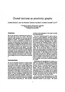
applied directly to compare similarities between items, or within a more general scheme such as clustering and ordering. Moreover, measuring proximities can help to characterize the global structure of a network by showing how closely coupled it is. However, while proximity measurement is well-understood for attribute-based, multivariate data, the situation is not as clear for objects in networks. Measuring proximities between entities or groups of entities in networks is an important and interesting task. Proximities can predict connections in a social network which have not been made yet [20, 23]. In a network with missing data, proximities potentially give evidence of links that have been removed or cannot be observed. Another popular way of using proximities is to find clusters or communities of entities in a network that behave similarly or have some commonality [11, 13]. Measuring proximity in networks is inherently more difficult and globally-oriented than it is with typical multivariate data. To calculate proximity for network objects, we must account for multiple and disparate paths between the objects. Unlike proximity measurement in multivariate data, which usually relies on a direct comparison of two relevant objects, calculating network proximity requires working with the network that lies between the two objects. Therefore, explaining network-proximity involves showing significantly more information. Recent work by Faloutsos et al [10] introduced connection subgraphs– small portions of a network that capture the relationships between two of its objects. Such subgraphs are closely related to the problem of measuring and explaining network proximity. In this study, which was largely inspired by Faloutsos et al, we introduce a novel way of measuring proximity between network objects that generalizes the previous approaches and provides certain advantages. We develop a new measure of proximity between network objects which has an intuitive interpretation based on random walks. This proximity measure can be readily “extracted” and visualized in the form of a proximity graph, and we describe different ways of visualizing the results. We explain how the proximity measure is easily generalized to find proximities between an arbitrary number of objects. Finally, we apply our methodology to four real data sets, each demonstrating a different strength of the methodology. As an example of the proximity graphs we produce, consider Figure 1, which represents the proximity graph between Meryl Streep, Judy Garland and Groucho Marx in the online movie database IMDB. The graph shows subcommunities of performers and their interrelationships. Readers may query this database and create their own proximity graphs on the web page at http://public. research.att.com/˜volinsky/cgi-bin/prox/prox. pl. An earlier version of this paper appeared in the proceedings of

Meryl Streep 3958

Jack Nicholson 4985

9.0

Jack Valenti 2266

7.0

Frank Sinatra 7625

24.0 10.0

8.0

22.0

7.0

13.0 Bob Hope 7828 5.0

Jessica Lange 2583 5.0

28.0

5.0

5.0

Harpo Marx 1476

7.0 6.0 6.0

5.0 29.0 5.0 5.0

Chico Marx 1153 30.0

10.0

53.0

Bing Crosby 11.0 8.0 5456 Judy [I] Garland 3189

11.0 5.0

12.0 7.0

11.0

5.0

Groucho Marx 5.0 1629

Jimmy Durante 2564

9.0

5.0

Clark Gable 4664

Figure 1: Extraction of proximity graph between Meryl Streep, Judy Garland and Groucho Marx in IMDB.com data. Edge weights are the number of co-occurrences in the IMDB data. CFEC=4.88e-2. Subgraph captures 97.8% with maxsize = 12. the ACM KDD-2006 conference [18]. The major addition in this version is Section 7 that discusses practical applications. The applications include link prediction, community detection, and estimation of values associated with nodes in a recommendation system. Additionally, we elaborate on the experimental results that were previously reported.

2.

THE QUEST FOR PROXIMITY

Proximity is a subtle notion, whose definition can depend on a specific application. Usually the notion of proximity is strongly tied to the definition of an edge in the network. In a network where links represent phone or email communication, proximity measures potential information exchange between two non-linked objects through intermediaries. Where edges represent physical connections between machines, proximity can represent latency or speed of information exchange. Alternatively, proximity can measure the extent to which the two nodes belong to the same cluster, as in a co-authorship network where authors might publish in the same field and in the same journals. In other cases, proximity estimates the likelihood that a link will exist in the future, or is missing in the data for some reason. For instance, if two people speak on the phone to many common friends, the probability is high that they will talk to each other in the future, or perhaps that they already communicate through some other medium such as email. There are many uses for good proximity measures. In a social network setting, proximities can be used to track or predict the propagation of a product, an idea, or a disease. Proximities can help discover unexpected communities in any network. A product marketing strategist could target individuals who are in close proximity to previous purchasers of the product, or target individuals who have many people in close proximity for viral marketing. In what follows, we formalize the notion of proximity by sequentially refining a series of candidate definitions, starting with the simplest one: shortest path. Notationally, we assume we have a graph G(V, E), where the “network objects” are nodes (V ) and the links between them are edges (E). The weight of edge (i, j) ∈ E is denoted by wij > 0 and reflects the similarity of i and j (higher weights reflect higher similarity). For non-adjacent nodes, (i, j) ∈ / E we assume wij = 0. Each node is associated with a degree greater or equal to the sum of the edge weights coming out P of that node. Usually, equality applies here such that degi = j:(i,j)∈E wij . Sometimes we will equivalently refer to “distance”

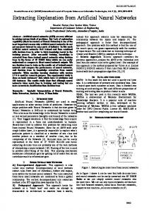
measures, which are the opposite of “proximity” measures - low distance equates to high proximity. Unless stated otherwise, we are measuring proximity between two nodes s and t. Graph-theoretic distance The basic definitions we need for network proximity are taken from graph theory. The most basic one is the graph theoretic distance, which is the length of the shortest path connecting two nodes, measured either as the number of hops between the two nodes, or the sum of the edge lengths along the shortest path. The main rationale for considering graph theoretic distance is that proximity decays as nodes become farther apart. Intuitively, information following a path can be lost at any link due to the existence of noise or friction. Therefore two nodes that are not connected by a short path are unlikely to be related. Distance in graphs can be computed very efficiently [7]. However, this measure does not account for the fact that relationships between network entities might be realized by many different paths. In some instances, such as managed networks, it may be reasonable to assume that information between nodes is propagated only along the most “efficient” routes. However, this assumption is dubious in real world social networks, where information can be propagated randomly through all possible paths. For example consider Figure 2, which shows several different possible connections between s and t. For i = 1, 2, 3, the graph-theoretic distance between nodes si and ti is 2, yet we have different conclusions about their proximity. One would likely conclude that s2 is closer to t2 than s1 is to t1 , because they have more “friends” in common. And s3 and t3 are only connected through a node with high degree, which might indicate that they are not close at all (as in two people who both call a very common toll free telephone number). Ideally, proximity should be more sensitive to edges between low-degree nodes that show meaningful relationships, and take into account multiple paths between the nodes. !$

*$

"$

*% !#

"# *# &# &%

&$ *)

!% &'

"% &)

&( !)

+$

+#

+%

")

!(

,$

,#

,%

"(

Figure 2: A collection of graphs with all edge weights equal 1 Network flow Consider another concept from graph theory– maximal network flow [7]. Here we assign a limited capacity to each edge (e.g. one proportional to its weight) and then compute the maximal number of units that can be simultaneously delivered from node s to node t. This maximal flow can be taken as a measure of s-t proximity. It favors high weight (thus, high capacity) edges and captures the premise that an increasing number of alternative paths

between s and t increase their proximity. Referring again to Figure 2 we can deliver twice as many units between s2 and t2 than s1 − t1 , thereby gaining from the alternative paths. However, maximal flow disregards path lengths, so that we get the same maximal flow between s4 and t4 as between s1 and t1 . Also problematic with this definition is that the maximal s-t flow in a graph equals the minimal s-t cut– that is, the minimal edge capacity we need to remove to disconnect s from t [7]. In other words, the maximal flow equals the capacity of the bottleneck, making such a measure less robust. For example, the maximal flow between s5 and t5 is 1, equal to the maximal flow between s4 and t4 , despite the added pathways in s5 − t5 . From the information-flow viewpoint, added pathways create more opportunity for the information to pass from s to t, and hence the points should be closer. The network flow measure is too dependent on the bottleneck, and does not account for multiple paths or node degrees. Effective conductance (EC) A more suitable candidate comes from outside the classical graph-theory concepts– modeling the network as an electrical circuit by treating the edges as resistors whose conductance is proportional to the given edge weights. This way, higher weight edges will conduct more electricity. Descriptions are found in standard references [4, 9]. When dealing with electrical networks, a natural s-t proximity measure is found by setting the voltage of s to 1, while grounding t (so its voltage is 0) and solving a system of linear equations to estimate voltages and currents of the network. The computed delivered current from s to t, is also called the effective conductance, or EC. Effective conductance appears to be a good candidate for measuring proximity. It has been applied previously in graph layout algorithms [6], and to compute centrality in social networks [5]. Faloutsos et al [10] also consider EC in their study of connection subgraphs. An important advantage is that it accounts for both path length (favoring short paths, like graph-theoretic distance) and alternative paths (more are better, like maximal flow), while avoiding dependence on a single shortest path or bottleneck. An appealing property of EC is that it has an equivalent intuitive definition in terms of random walks. Let’s denote effective conductance between s and t as EC(s, t). Also, let Pesc (s → t) be the escape probability, the probability that a walk starting at s reaches t before returning to s. It is known [9] that EC(s, t) can be expressed as: EC(s, t) = degs · Pesc (s → t) = degt · Pesc (t → s)

(1)

Effective s-t conductance is the expected number of “successful escapes” from s to t, where the number of attempts equals the degree of s. From an information-sharing viewpoint, this interpretation captures the essence of unmanaged, self-organizing networks when information, or general interactions, may pursue random routes rather than following well planned routes. Consequently, the escape probability decreases if long paths must be followed, because when tracking a long path from s to t there is a increased chance of returning to s before reaching t. EC also has a monotonicity property, courtesy of Rayleigh’s Monotonicity Law [9]. This law states that in an electrical resistor network, increasing the conductance of any resistor or adding a new resistor can only increase the conductance between any two nodes in the network. In our context it means that each additional s-t path contributes to an escape from s to t, increasing EC. Referring back to Figure 2, this implies that EC(s5 , t5 ) > EC(s4 , t4 ), and EC(s2 , t2 ) > EC(s1 , t1 ), which is intuitive. While monotonicity it is desirable in some cases, in others it contradicts our desired notion of proximity. As an example, again in Figure 2, EC(s1 , t1 ) = EC(s3 , t3 ). In terms of random walks,

the nodes of degree 1 emanating from node a4 to b1 , . . . , b6 have no effect on escape probability, and therefore EC, because any walk following these edges is going nowhere and will eventually backtrack to a4 . Such backtracking means the random walk can make an unlimited number of attempts to reach s or t through these highdegree nodes without affecting EC. Real-world datasets tend to follow power laws in their degree distribution [1] and have many nodes of degree 1, so this shortcoming can be quite significant. In our view, links into degree-1 nodes indicate real relationships, and should not be neglected when measuring proximity. Sink-augmented effective conductance Faloutsos et al [10] modify the EC model by connecting each node to a universal sink carrying 0 voltage. Thus, the universal sink competes with t in attracting the current delivered from s. It has the effect of a “tax” on every node that absorbs a portion of the outgoing current. Consequently, this forces all nodes to have a degree greater than 1, so the issue we mentioned with degree-1 nodes can no longer exist. Considering the universal sink from the random-walk perspective, it gradually overwhelms the walk, as after each step there is a certain probability that the walk will terminate in the universal sink. The universal sink model requires a parameterization of the sink edges, to determine how much of the flow through each node is taxed. Understanding how such a parameter influences the computed proximities is difficult. A more important shortcoming of the universal sink is that it does not guarantee monotonicity. As the network becomes larger, adding paths between s and t, the proximity between s and t typically decreases, approaching zero for large networks. The reason is that every new node must provide a direct link to the sink, while usually providing no direct link to the destination t. Therefore, an increasing number of nodes strengthens the sink to the point that t is not able to compete for delivered current. This introduces a counterintuitive size bias: the proximity between s and t calculated from a graph will typically be significantly increased when looking at a small subgraph of that graph. One immediate implication of this size bias artifact is that it thwarts our goal of proving (or explaining) proximity using a small representative subgraph; since the proximity value strongly depends on the graph size, each selected subgraph will convey a different proximity value, usually much larger for smaller subgraphs. Computing optimal subgraph size or understanding how to normalize for graph size is unclear. Moreover, this dependency on size makes proximity comparisons across different pairs uninterpretable. Therefore, we assert that while sink-augmented current delivery solves many of the problems previously mentioned, its non-monotonic nature is unsuitable for measuring proximity. In the following section, we introduce a proximity measure, cyclefree effective conductance, which provides advantages over the aforementioned methods, and has an intuitive random walk interpretation.

3. CYCLE-FREE EFFECTIVE CONDUCTANCE (CFEC) Our approach for measuring proximity is based on improving the effective conductance measure. To this end, we consider the random-walk interpretation. Before we give exact definitions, some notation is necessary: in the random walk, a probability of transiwij tion from node i to node j is pij = deg . Thus, given a path i P = v1 − v2 − · · · − vr , the probability that a random walk starting at v1 will follow this path is given by: Prob(P ) =

r−1 Y i=1

wvi vi+1 degvi

(2)

At times we will refer to the weight of a path P , which we will define as: Wgt(P ) = degv1 · Prob(P )

(3)

These definitions also apply to directed graphs. Recall that Equation (1) relates effective conductance to the escape probability. Escape probabilities are characterized by a walk that will make an unlimited number of trials to reach an endpoint– s or t. Meanwhile, it might backtrack and visit the same nodes many times. We argued above that this is problematic when measuring proximity, as it does not consider any such paths to be distracting ones that lower s-t proximity. We fix this problem is by considering cycle-free escape probabilities, which disallow backtracking and revisiting nodes: D EFINITION 3.1. The cycle-free escape probability (Pcf.esc (s → t)) from s to t is the probability that a random walk originating at s will reach t without visiting any node more than once. From the information sharing viewpoint it means that information flows randomly in the network, while already known information has no contribution to the overall flow. This way, for example, high degree nodes will distribute their information among all their neighbors, but sending information in the “wrong” direction (not leading to t) is a wasted effort, which cannot be fixed by a later backtracking. Consequently we replace effective conductance by cycle free effective conductance, which is defined, similarly to Equation (1), as: ECcf (s, t) = degs · Pcf.esc (s → t)

(4)

As previously, we can take ECcf (s, t) as the expected number of walks completing a cycle free escape from s to t, given that degs such walks were initiated. Henceforth, we abbreviate cycle-free effective conductance as CFEC. In undirected graphs, random walks have the reversibility property [9] resulting in the equality: CFEC(s, t) = CFEC(t, s) How useful is CFEC-proximity? We assert that CFEC serves well as a proximity measure, because it integrates advantages of previous candidates while solving shortcomings. Before we test CFEC against the previously proposed criteria, we note the following equalities. Let R be the set of simple paths from s to t (simple paths are those that never visit the same node twice):

+$

!

X

Prob(R)

"

Another desired property of a proximity measure is that it favors pairs that are connected by multiple paths. This property, too, is inherent to CFEC, being a sum of (positive) weights of all alternative paths. For example, for the graph family in Figure 4, CFEC(s, t) proximity is k/2, growing with the number of alternative paths. *-

!

" *# *$

Figure 4: A family of graphs characterized by the number of s-t paths Moreover, unlike graph-theoretic and maximal-flow distances which are dependent respectively on a shortest path and the max cut, CFEC relies on all s-t paths, so each edge on any such path makes a contribution to the measured value. We now address the issue of degree-1 nodes and, in general, dead end paths. Recall that such distracting paths were neglected by the other proximity measures, because of their monotonicity property. However, with CFEC any simple path leading from s to a node other than t must reduce the probability of escaping to t. For example, in Figure 5, the degree-1 nodes dilute the significance of the s − a, a − t links, yielding 1/(k + 2) CFEC proximity for this family of graphs. Of course, this is also tightly related to discounting the effect of high-degree nodes, as any single path passing through a node has a probability which is inversely proportional to the degree of that node. &# &-

&$ *

"

(5)

R∈R

Similarly, by multiplying by the degree: X CFEC(s, t) = Wgt(R)

+-

Figure 3: A family of s-t paths

!

Pcf.esc (s → t) =

+#

Figure 5: A family of graphs with varying degree of a (6)

R∈R

It is clear that a cycle-free escape must proceed along a simple path from s to t, so Equation (5) merely sums the probabilities of all possible disjoint events. We will return to these equations later, when dealing with how to compute CFEC. However, for now they will aid us in studying CFEC’s characteristics. First, we require a proximity measure that favors short paths, as two remote nodes are unlikely to be in proximity. As evident from Equation (5), CFEC strongly discourages long paths as the probability of following a path decays exponentially with its length. For example, for the family of graphs shown in Figure 3, s-t proximity decays exponentially with their distance, CFEC(s, t) = 2−k .

The correct treatment of dead end paths means that the CFEC measure is not monotonic with respect to edge addition; e.g., adding degree-1 nodes decreases proximity. However, we avoid the aforementioned size bias, where subgraphs have smaller proximity values than their corresponding supergraph. We accomplish this by constructing subgraphs in a special way which preserves monotonicity, as we explain now. It is reasonable to expect the most accurate proximity value to be the one measured on the full network. Therefore, when we measure proximity on increasingly larger subgraphs, we expect it to steadily converge towards its more accurate value. To this end, the operation we use for cutting a subgraph from the full graph preserves node degrees. Formally, given a graph G(V, E) and a subset Vˆ ⊂ V , ˆ Vˆ , E), ˆ where E ˆ = {(i, j) ∈ then the subgraph induced by Vˆ is: G(

E | i, j ∈ Vˆ } and degrees are unchanged. That is, for each ˆ def G i ∈ Vˆ : degG i = degi , where superscripts indicate the respective graph. Here, we took the liberty to use node degrees that are greater than the sum of respective adjacent edge weights (consistent with our definition of degree in Section 2). In essence, each node has a self loop whose weight ensures that each degree equals the sum of adjacent edge weights. Preservation of original degrees ensures that CFEC proximity measured on a graph cannot be smaller than the CFEC proximity measured on a subgraph thereof: according to the definition of CFEC in Equation (6), any simple s-t path that ˆ must have the same weight (or probability) as in the full exists in G graph G. However, there might be additional s-t paths that exist only in G, which will lower CFEC proximity when measured on ˆ Therefore CFEC proximity is a monotonic series the subgraph G. under this subgraph operation. This series is tightly bounded from above by the proximity measured on the full graph. In other words, when measuring proximity on a subgraph of the full network, the larger the subgraph, the more accurate the measurement, a desirable property. In practice, we found that measuring proximity on an s-t neighborhood requires only a small fraction of the full graph. Further increasing the neighborhood size yields diminishing improvements. When an accurate proximity measure is needed, one cannot lose accuracy by working with the largest possible network. On the other hand, CFEC proximity can often be explained by small subgraphs, in the sense that if we measure a certain proximity value on a very small subgraph, then this value is a provable lower bound of the accurate proximity value. We will show later that experimentally, a very significant portion of the proximity can usually be explained by subgraphs with fewer than 30 nodes. This strongly suggests that the connection subgraphs of Faloutsos [10], and our proximity graphs, are very effective in capturing the relationships that determine CFEC proximity. Later (Subsection 5.1) we will see that this allows us to assign confidence scores to the proximity graphs, reflecting how well they describe full proximity. Directed graphs differ from undirected graphs in having asymmetric connections, so an edge i → j can be used only for moving from i to j, but not vice versa. Interestingly, in contrast with electrical resistor network models, cycle-free effective conductance naturally accommodates directed edges, as its underlying notions remain well defined for directed graphs. An interesting issue is the emerging asymmetry CFEC(s, t) %= CFEC(t, s). In fact, one can view it as a mere reflection of the inherent asymmetry of directed edges, which, also exist in the graph-theoretic distance - the other proximity measure that deals with edge directions. If needed, one can remove this symmetry by taking the sum CFEC(s, t) + CFEC(t, s) or the product CFEC(s, t) · CFEC(t, s) as the s-t proximity.

4.

COMPUTING CYCLE-FREE ESCAPE PROBABILITY

We are not aware of any efficient algorithm for computing CFEC proximity exactly. However, we can efficiently find accurate approximations. Fortunately, we may not even need much accuracy– experiments show that even estimating merely the order of magnitude of proximity may suffice since proximity values appear to be lognormal distributed (Figure 10). The basis for our approximation is Equation (5): X Pcf.esc (s → t) = Prob(R) R∈R

We can estimate this value using only the most probable s-t paths.

In all our experimental datasets, we consistently found that path probability falls off exponentially. If we order simple s-t paths by probability, the 100th path is typically a million times less probable than the first. Based on empirical results, the probability of paths drops fast enough that the low probability paths cannot sum to any significant value. Therefore, we estimate CFEC(s, t) by restricting the sum in Equation (5) to the k most probable simple paths Rk , where this set is determined by some threshold. Usually we stop when the probability of the unscanned paths drops significantly below that of the most probable path (e.g. below a factor of 10−6 ). Thus we need an algorithm to find simple s-t paths in order of decreasing probability. To this end, we first transform edge weights into edge lengths, establishing a 1-1 correspondence between path probability and path length. For each edge (i, j) we define its length, lij to be: ! wij lij = − log p (7) degi · degj Using these edge lengths, path lengths correspond to path probabilities via the equation: Prob(R) = C · e−length(R) q degt where R is some s-t path, and the positive constant C is deg . s Therefore, the shortest path is the most probable path; the second shortest path is the second most probable, and so on. Our solution involves the k shortest simple paths problem, a natural generalization of the shortest path problem, in which not one but several paths in order of increasing length are sought. Interestingly, Katoh et al [17] describe an efficient algorithm for undirected graphs, with running time linear in k and log-linear in the graph size: O(k(|E| + |V | log |V |)); Hadjiconstantinou and Christofides present additional implementation details [14]. We employ this algorithm to find the shortest (most probable) simple paths. Paths of monotonically increasing length are generated successively. (As mentioned, we stop the search when the path probability drops below a certain threshold. In our implementation this is ! = 10−6 of the probability of the first, most probable path.) The number k of such computed paths is usually a few hundred. Then, the estimated CFEC proximity is: X CFEC(s, t) = Wgt(R) (8) R∈Rk

5. EXTRACTING PROXIMITY THROUGH PROXIMITY GRAPHS The computed CFEC proximity value depends on the full network. Therefore, explaining the proximity value or convincing a user of its validity can be complex. Nonetheless, frequently our ability to use proximity values and act upon them depends on our ability to understand the structure that drives them. So one of our main goals is to find ways of extracting and explaining proximity using small, easily visualized subgraphs, which we call proximity graphs. Practically, we are looking for small subgraphs of the original network, such that the s-t CFEC proximity measured on this subgraph is close to that measured using the full network. This is related to the connection subgraphs structure proposed by Faloutsos et al [10], extracted to represent the relationship between two nodes. A distinction from Faloutsos et al [10] is that we work here in the context of explaining a specific CFEC proximity value. Fortunately, the cumulative nature of CFEC proximity, as expressed in Equation (8) eases the task. We store the k paths that

were used for computing the proximity value, so these paths serve as the building blocks of the connection subgraph. Formally, we have a sorted series of paths: Rk = P1 , P2 , . . . , Pk , such that Wgt(Pi ) ! Wgt(Pi+1 ). We form the connection subgraph by merging a subset of Rk . The easiest solution would be to merge the most probable paths, without exceeding some fixed bound on the numberSof nodes B > 0. That is, we compute the maximal r for which | ri=1 Pi | " B, and then define the connection subgraph S as the subgraph induced by the union of the first r paths ri=1 Pi . This simple approach is plausible, as we have found experimentally in our datasets. However, it fails to account for overlaps between paths. Overlapping paths, which share common nodes, have the advantage of increasing the captured proximity while using fewer nodes. Therefore, we can do better by looking at general subsets of Rk rather than considering only prefixes thereof. In which subset of Rk we are interested? One possibility is to find a subset that solves (A1) Extract a subgraph with at most B nodes that captures maximal s-t proximity Dually, instead of fixing size, we can fix the desired amount of captured proximity, so the subset will solve: (A2) Extract a minimal-sized subgraph that captures an s-t proximity value of at least C However, optimizing either (A1) or (A2) can yield inefficient solutions, due to the arbitrariness of B or C. For example, when solving (A1), it might be that by replacing B with B + 1 we could have captured much more proximity. Or, when solving (A2), maybe by taking C − 1 instead of C we could have significantly reduced the subgraph size. Hence, we prefer working with the following formulation that achieves an efficiently balanced solution by considering CFEC-per-node: ˆ Vˆ , E) ˆ that maximizes the (A3) Extract a subgraph G( ratio: ”α “ ˆ CFECG (s, t) (9) &Vˆ & ˆ ˆ The conHere, the superscript G indicates measuring CFEC on G. stant α ! 0 determines our preference in the size vs. proximity tradeoff: The greater α is, the more we favor the numerator, maximizing the captured proximity. Thus, when α = 0 only the subgraph size matters, and an optimal solution will be a shortest path (measured by number of nodes). Similarly, in the other extreme case when α = ∞, size becomes irrelevant, so an optimal solution merges all k available paths. As shown experimentally, we find 5 " α " 10 to be effective. Note that by using a ratio, the inefficiencies mentioned above cannot exist– an optimal ratio cannot allow a small increase in the denominator (size) to significantly increase the numerator (captured proximity), or vice versa. In implementation, for numerical reasons we recommend using the logarithm of this ratio as a proxy for its actual value, which is important when α is large. Also, in the denominator, it may be reasonable ˆ (or &E& ˆ + &Vˆ &) since high edge density to replace &Vˆ & with &E& interferes with the readability of the graph layout (though we have not yet explored this experimentally). An obvious question is how to find a subset of Rk that solves the above problem. Solving (A1)–(A3) is NP-hard, as they are reducible from the closely related Knapsack problem [12] (with the main difference that here we need to account for possible overlaps

Function PathMerger (P1 , P2 , . . . , Pk ) % Input: a list of paths sorted by decreasing weight Stack ← ∅ BestSubset ← ∅ P W eights ← ki=1 Wgt(Pi )

for i = 1 to k do W eights ← W eights − Wgt(Pi ) for Subset ∈ Stack ∪ {∅} do N ewSubset ← Subset ∪ Pi N ewSubset.wgt ← Subset.wgt + Wgt(Pi ) if Score(N ewSubset.wgt + W eights, &N ewSubset&) > Score(BestSubset.wgt, &BestSubset&) then Stack.push(N ewSubset) if Score(N ewSubset.wgt, &N ewSubset&) > Score(BestSubset.wgt, &BestSubset&) then BestSubset ← N ewSubset end if end if end for return BestSubset end Function Score (weight, size) α return weight % See Equation (9) size end Figure 6: The branch-and-bound path merging algorithm between the paths in addition to their size and weight). It is very unlikely we can devise a polynomial-time algorithm for solving these problems. Consequently, we suggest two heuristic approaches. The first is an exact branch-and-bound (B&B) algorithm. Since this might take exponential time, we may have to prematurely terminate the search. In that case, we take the best intermediate solution discovered by B&B and try to improve it by an agglomerative polynomial-time algorithm. The branch and bound algorithm for optimizing (A3) Recall that we ordered paths by their weights. Accordingly, we scan all subsets of Rk in lexicographic order, so we scan all subsets containing Pi before completing the scan of subsets containing Pi+1 . This way we target more promising subsets (based on total weight) first. A full scan would loop through all 2k possible subsets and find an optimal one. However, we can significantly reduce running time by pruning subsets that are provably suboptimal. To this end, during the scan we record the best subset found so far. Then, for every new subset, we check whether under the most optimistic scenario it can be a part of an optimal solution. This check is done by adding the weights of all subsequent paths to the weight of the current subset, while assuming that the size of this subset would not be increased at all. If even after this operation the subset’s score (according to Equation (9)) is lower than the current best one, we prune the search, skipping this subset and all subsequent subsets containing it. Detailed pseudocode is given in 6. When the B&B algorithm terminates early we need to switch to the greedy agglomerative optimizer. This algorithm starts with the k sets {P1 }, {P3 }, . . . , {Pk }. To take best advantage of the result of the B&B algorithm, we merge all sets whose union is the result returned by the B&B algorithm into a single subset. Then, the algorithm iteratively merges the two sets maximizing (9) (replacing two sets by their union), till a single set remains. During the process

we record the best set found, which is returned as the final result. In experience, we often find an optimal solution with the branchand-bound algorithm, and even when the agglomerative optimizer is invoked, usually it cannot improve the B&B result. Also, our implementation allows setting an upper bound (maxsize) and a lower bound (minsize) to limit the proximity graph’s size.

5.1 Assessing proximity graphs Proximity graphs created by our method are aimed at capturing maximal proximity with few nodes. By definition, the CFECproximity captured in these subgraphs must be lower than the full CFEC-proximity measured on the whole network. In fact, the captured CFEC is easily computed by taking the sum of weights of those paths whose merge created the connection subgraph. Hence, we can use the CFEC-proximity to assess the quality of the subgraphs, by reporting the percentage of captured proximity. For example, a connection-subgraph with a 10% score is not very informative as it captures only a small fraction of the existing relationships. On the other hand, a subgraph with a 90% or higher score shows most of the available proximity. Moreover, proximity values between different pairs of objects within the same graph are directly comparable. The ability to compute, optimize, and analyze this score is a key contribution of our proposed technique.

5.2 Multiple endpoints Another benefit of our method is that it is easily extended to show relationships between more than two endpoints. The only change to the algorithm is the way we construct the set of paths Rk . When multiple endpoints exist, we are no longer looking for shortest paths among two endpoints but for the broader set of shortest paths connecting any two of the given endpoints. This is achieved by a straightforward generalization of the k simple shortest paths algorithm that finds simple shortest paths connecting any two members of a given set of nodes. Time complexity is virtually unaffected, being for l endpoints: O((k + l2 )(|E| + |V | log |V |)). No other modification is necessary to the algorithm. There are some important details about handling queries with multiple endpoints. In particular, we do not require that the proximity subgraph connects all endpoints, only those that make a sufficient contribution to the overall proximity value. Only relevant endpoints appear in the extracted subgraph. Thus, one has the flexibility to query proximity relations among many endpoints without being concerned about which of them is really relevant. Then, our algorithm prunes the unrelated endpoints, allowing the user to concentrate on the most useful relationships. Alternatively, one could enforce that all endpoints be connected. In some applications, users might require such behavior. This is easily achieved by post-processing to insert each of the unconnected endpoints using the most probable (shortest) path connecting it to the computed proximity subgraph.

5.3 Directed edges As mentioned above, CFEC-proximity is also general enough to handle directed edges. Naturally, this is also valid for the connectionsubgraph construction algorithm, as it deals with entire paths regardless of the direction of their edges. Obviously, if edges are directed, the algorithm that produces the k shortest paths must be changed to account for edge directions. This increases running time. The algorithm we chose (by Katoh et al [17]) works only on undirected graphs. An algorithm for computing the k simple shortest paths on a directed graphs was described by Hershberger et al in [16]. Its time complexity is O(k|V |(|E| + |V | log |V |)) but Hershberger et al claim that we rarely encounter this worst-case behavior,

and the average case running time is only O(k(|E| + |V | log |V |)), which is comparable to the undirected case.

6. WORKING WITH LARGE NETWORKS Some of the databases we work with are huge. The DBLP cocitation graph has over 400,000 authors; the IMDB movie-actors connection graph has about a million nodes and 4 million edges; a telephone call detail database may have hundreds of millions of nodes. The Yahoo Instant Messenger database is even larger, with about 200 million nodes and 800 million edges [19]. Computation on such large networks can exceed typical time and space resources. However, in practice, only a tiny fraction of the network makes a significant contribution to any computed proximity value. This is supported by the efficacy of very small connectionsubgraphs to explain proximity, as we report in Section 7. Therefore, we can work only on a portion of the full network that includes the relevant information. To this end we compute a conservative estimate of this portion, which is usually a tractable subgraph containing a few thousand nodes. Then, the proximity value is computed on this subgraph, and the much smaller connection subgraph is extracted from it. Note that here we are only interested in a fast, coarse approximation of the relevant portion of the full network, unlike the more precise computation that extracts the connection subgraph. Faloutsos et al [10] deal with similar issues in computing connection subgraphs. They named the reduced subgraph on which their connection subgraph is computed a candidate graph. We adopt this nomenclature. It appears that the tight relationship between our candidate graph and measured CFEC proximity allows aggressive pruning of its size, while still maintaining sufficient connectivity structure. Growing candidate graphs via {s, t} neighborhoods Let us assume that we are computing the proximity between two nodes s and t. Cases involving more than two endpoints will be handled analogously. The first stage in producing the candidate graph is to find a subgraph containing the highest weight paths originating at either s or t. Recall that the weight of a path is defined by Equation (3): Wgt(P ) = degv1 · Prob(P ). By transforming edge weights into edge lengths as described in Equation (7), the problem becomes: find a subgraph containing shortest paths originating at either s or t. Equivalently, our object is to expand the neighborhoods of s and t. This is done by the standard Dijkstra’s algorithm [7] for computing shortest paths on graphs with non-negative edge lengths. This algorithm finds a series of nodes with increasing distance from {s, t}. Note that to make the algorithm efficient on a huge graph, we assume an indexing mechanism that allows us to efficiently access the neighborhood of a given node. Determining neighborhood size When do we stop growing the {s, t} neighborhoods? Assume that the highest weight, that is shortest length, s-t path is P of length L. This path will be discovered by the algorithm when the {s, t} neighborhoods grow enough to overlap. Since such an overlap occurs, the path P passes within the neighborhood that was created. Recall that CFEC proximity is computed using the k shortest paths, such that the (k + 1)th path is the first path whose weight drops below ! times the weight of the first path. After transforming weights into lengths, we know that paths longer than L − log(!) are not useful. Therefore we should expand the neighborhood until it covers all s-t paths shorter than L − log(!). Consequently, we are interested only in nodes whose distance from either s or t is at most (L − log(!))/2. To summarize, {s, t} neighborhoods are expanded until they overlap. At this point we learn L - the length of the shortest s-t path. Then, we continue by expanding the (L−log(!))/2-neighborhoods

of both s and t. Every significantly weighted s-t path must go through this neighborhood. In practice, these (L − log(!))/2-neighborhoods might be too large. In these cases we stop extending the neighborhood when its size reaches a predetermined limit, typically several thousand. Pruning the neighborhood Interestingly, the created neighborhood can be significantly pruned. This is true regardless of whether we completed generating the full (L − log(!))/2-neighborhoods or stopped earlier. Let us denote by dist(i, j) the length of the shortest path between i and j (the graph-theoretic distance). Observe that if dist(s, i) + dist(t, i) > β then any s-t path going through i must be longer than β. Therefore, we compute dist(s, i) and dist(t, i) for each i in the neighborhood. Then we exclude from the neighborhood any i for which dist(s, i) + dist(t, i) > L − log(!), as no s-t path of appropriate length can pass through such i. Graphically, this pruning takes the two “circles” centered at s and t and transforms them into an “ellipse” with two foci– s and t– defined by the equation dist(s, i) + dist(t, i) " L − log(!). Empirically, we have found this pruning to be very effective, usually removing most nodes in the neighborhood. Finally, we take the graph induced by the pruned neighborhood as our candidate graph, calculate CFEC proximity between the objects of interest with respect to this graph, and extract the proximity graph which best captures that proximity.

7.

APPLICATIONS

We tested the CFEC proximity measure on several large network datasets. Each application highlights specific features of the proximity measure. The test datasets were: 1. Telecommunications Data (Phone) The U.S. telephone network has hundreds of millions of phones; the calls between these phones can be viewed as a massive network. AT&T has a record of calls carried on its network, which is on the order of hundreds of millions per day, and the number of nodes (telephone numbers) is of the same order of magnitude. Typically, an edge in this graph indicates that there has been at least one call between the two phone numbers in the last time period t, often set to 30 or 90 days. We put a weight on the edges representing the total communication time. 2. Co-authorship (DBLP) The DBLP database (http://dblp. uni-trier.de/ is an online bibliography of computer science journals and proceedings [8]. The data from the bibliography is freely available and can be used to create a network of co-authorship, where the nodes in the network are authors, and the links indicate co-authorship. Link weight indicates how many papers two researchers published together. 3. Movie Actors (IMDB) The Internet Movie Database (www. imdb.com)provides meta-data on movies and television shows including the actors who appeared in those shows. From this data, one can generate a network where the nodes are actors and the links represent actors who appear together in at least one show. Weights on the links indicate multiple appearances. 4. Movie Ratings (Netflix) In 2006, the internet movie rental company Netflix released a large data set as part of a contest to see if anyone could improve upon their movie recommender system. The data consisted of ratings of movies from almost 500,000 Netflix users. We created a network from this data where links represent movies co-rated by the same user and these links have two attributes: support, or the number of users who co-rated these movies, and a similarity score indicating how similar the scores are when co-rated. Although

proximities could be useful in recommender systems, in this paper we are simply exploring the utility of this new proximity measure. More comprehensive techniques for building recommender systems for the Netflix dataset are described in [24, 2]. Table 1 show some basic statistics about the datasets, along with some average features for proximity graphs calculated on a random sample of pairs from each dataset. Some interesting features emerge. In comparing DBLP and IMDB, for instance, we see that DBLP is less dense, with considerably fewer edges per node. This corresponds to a smaller percentage of pairs for which we are able to find connecting paths, but interestingly the paths found tend to be much shorter, indicating a network consisting of many small clusters. In contrast, in the much larger telephone call network, we find paths between 90% of randomly chosen node pairs, despite an extremely low density. The phone network also has a relatively small median proximity graph size, and high proximity values (although since these values depend on the scale of the edge weights, they are not directly comparable across datasets). So the phone network, despite it being vast and sparse, actually connects most of the communications universe. The Netflix data is an interesting contrast. It is quite close to a complete graph, so measurements like shortest path and graph size are less relevant, yet the density of this graph brings up some different questions about the relationships between nodes, as discussed below. Value Nodes Edges Mean Degree Density Link? Median Prox SPath GSize

Phone ∼300M ∼1B ∼ 40" ∼ 0" 90 -6.5 5.8 20

DBLP 438K 1.2M 5 10−5 54 -7.4 4.4 28

IMDB 896K 47 M 104 10−4 77 -7.6 7.7 43

Netflix 17770 157.5M 17728 1 100 -3.9 1.0 2

Table 1: Statistics for four experimental data sets. The Prox column shows the mean log proximity value. Link? reports the percentage of pairs in the sample that had any path between them. SPath is the mean shortest path among pairs in the sample where a path was found. GSize indicates the median proximity graph size for those pairs. (for the Phone data, the " indicates that the mean degree and density were calculated for a sample of residential data points only, while the other measurements include all data.)

7.1 Exploring Properties of Proximity Graphs In our first example, we apply our proximity measure to the Phone data. For this exercise, we are interested in proximities between subscribers of a particular communications service. We have all records of communications between members of this group, as well as communications from this group to other members of the larger telecom network. Because there are many calls carried on other networks, there is a potential missing data problem which we ignore for the time being. Note that we have no access to content of the communication, simply a record that the communication occurred, and its duration. In addition, for research purposes we do not access any customer identifying data such as name or address. We can calculate CFEC proximity between any two members of this network readily, using the methods described earlier. We extract the candidate graph by growing neighborhoods from the

95 90 85

% Captured Proximity

100

which is small enough for readable visualization. From the bottom plot, we see that if the algorithm selects a smaller graph size, there is more variance in the amount of captured proximity. However, for all graph sizes, the mean (represented by the smoothing spline) is consistently around 95%. This indicates that the algorithm does a good job of balancing graph size against captured proximity.

80

two nodes of interest as described in Section 6, and then find the proximity graph using Equation (9). For the experiments below, we selected 2000 random pairs of telephone numbers to calculate the CFEC value. For 1808 (90%) of these pairs, we were able to find paths between them; the others did not have any known path between them, perhaps because they are low usage numbers, or perhaps due to the missing data problem. The parameter α (Equation (9)) allows the user to trade-off the desire for a small, visualizable subgraph for capturing more of the total proximity in the graph. To investigate this parameter, we calculated the percent of overall CFEC proximity captured in the subgraph. As α increases, so does the size of the subgraph, hence more of the available proximity will be captured. Figure 7 shows the results for our sample. Boxplots plotted at α = 1, 5, 10, and 50 show the percent of delivered current in the subgraph. A horizontal line is drawn at 95% for reference. For α = 10 about 3/4 of the subgraphs capture 95% of the CFEC proximity, and these graphs are relatively small (median=24 nodes, sd=16). If we bump up to α = 50, almost 100% of our samples capture 95% of the overall proximity, at the cost of larger subgraphs (mean=50, sd=32). We think α = 10 gives the best trade-off, yielding graphs small enough to be visualized, so we use this value in all subsequent analysis for the Phone dataset. For contrast, we also plot the analogous plot for the Netflix dataset, which is considerably denser. It is clear that α = 10 is not sufficient to provide captured proximity of 95% or more, probably because there are simply so many paths between nodes due to the density of the graph.

0

Phone

20

40

60

80

Size of Graph

% Captured Proximity

100

Figure 8: Plot showing size of proximity graphs and their relation to captured proximity. The top plot shows the distribution of graph sizes for our sample of 2000 pairs. The bottom figure plots graph size against the percent captured proximity, with a smoothing spline plotted through the data.

80 60 40 20 0 1

5

10

50

Netflix

% Captured Proximity

100 80 60 40 20 0 1

5

10

50

Figure 7: Boxplots showing % delivered proximity as a function of α for the Phone data and the Netflix Data. The box marks the space between the 25th and 75th percentiles of the distribution. In Figure 8, we explore how large the subgraphs need to be to capture a meaningful percentage of proximity. Looking at the resulting subgraphs for 2000 pairs using α = 10, we plot graph size against the percent overall captured proximity in the bottom figure. On top we plot a histogram showing proximity graph size. One can see that the majority of the proximity graphs have 50 nodes or less,

Another aspect worth investigating is the relationship between the CFEC proximity measure and the simple graph-theoretic measure of shortest path. Figure 9 shows this relationship for our sample. We plot the shortest path in the network for each pair in our sample, and compare it to the calculated proximity. The distribution of proximity is shown for each value of shortest path as a boxplot (the width of the boxplot is proportional to the number of pairs in that group). The graph clearly shows that our proximity provides different information than shortest path. The medians of the distributions (indicated by the line in the box) show an expected general trend; as the shortest path between two nodes increases, their proximity decreases. However, the amount of overlap of the boxplots indicate that there may be pairs that are farther apart by shortest path that have quite similar proximities. It is clear that a ranking of closest pairs would be very different using these two metrics. Another interesting fact about the data: the median of the shortest paths across our sample is 6, corresponding (perhaps coincidentally) to Milgram’s folkloric “six degrees of separation.”

7.2 Using Proximities for Link Prediction Proximities in a social network such as the Phone data can be viewed as a measure of social closeness. As such, one might hypothesize that this measure can predict who will call each other in the next time period. This is the so-called “link prediction” problem [20]. Here, we show the utility of CFEC in predicting future links in the network. We performed an observational experiment using

0.06 0.00 −14

−12

−10

−10

−8

−6

−4

−2

0

2

4

2

4

log(Proximity) for Non−Communicators

0.10 0.00

−15

Density

0.20

Log(Proximity)

−5

Density

0.12

log(Proximity) for Future Communicators

2

3

4

5

6

7

8

9

10

11

−14

−12

−10

−8

−6

−4

−2

0

Length of Shortest Path

Figure 9: Boxplots of log proximity for each value of shortest path distance. Boxes represent distance between the 25th and 75th percentile of the distribution.

Figure 10: Histograms comparing distribution of logarithm of proximity score for pairs of nodes that communicated (top) and those that did not (bottom).

the Phone data: at time t, collect proximities on a large set of random pairs of phone numbers who have no communication history, wait until time t + δ, then see which of those pairs communicate during (t, t + δ). We then compare the proximities for those that communicated with those that did not. If proximity has predictive value, we expect those that communicated in the test period to have had closer proximity at time t, before the test period began. Our experiment shows that proximity indeed seems to have predictive value. Figure 10 shows the distribution of the proximities for the communicators and the non-communicators. Those that ultimately made a phone call had log proximity values averaging −2.4, while those that did not have a call averaged −5.9. Similarly, the data suggest that two nodes with proximity greater than 1 (log proximity > 0) have a high probability to be future communicators. Kleinberg and Liben-Nowell [20] describe a thorough comparison of various similarity metrics to predict co-authorship from the arXiv database. The methods ranged from simple counts of common neighbors to more complex methods based on random walks and clustering. They found that the most successful measures were those that were robust to spurious connections between nodes, such as a one-time collaboration between authors in disparate fields. The CFEC measure has such robustness: paths traversing a spurious link will likely not reach the destination, since cycling back down that link is not allowed. Another such method based on random walks [26] uses the idea of occasional re-start of the random walk to find “center-piece subgraphs”. These subgraphs identify the most central nodes between a given set of nodes, a concept similar to our proximity graphs. We plan to compare our method with these competing methods in future work.

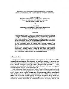
DBLP database allows us to find such clusters in computer science. Fig. 11 demonstrates our method’s ability to find communities and proximity graphs for more than two seed nodes. In this case, we search in the DBLP database for the well-known computer scientists Rivest, Adelman, Shamir and Knuth. The result shows the close relationship between the first three authors, and the connections with subcommunities of Israeli cryptographers and noted algorithms experts. Using proximities to find communities in databases like DBLP may also be useful for unaliasing, or correcting errors introduced when the same person shows up with two different labels [3]. By combining our work with string matching and other record linkage techniques, proximity graphs could contribute to a wide body of work on deduplication in databases [27]. Another way of approaching community detection is by defining and characterizing the community around a single node. To demonstrate this we use the Netflix data and build a community around a single movie m by calculating the proximities between that movie and all other movies in the network. By looking at the collection of movies that are closest to m, we can get a sense of whether it is part of a well-defined cluster of movies or is somewhat isolated in movie space. To demonstrate this, we selected two movies from the Netflix database: Barton Fink and Speed. These movies had near identical popularity, each scoring an average rating 3.5 (out of 5) with over 75,000 votes cast. However, Barton Fink is a quirkier movie, harder to characterize, and less accessible to a vast audience, while Speed belongs to the well-defined genre of action-thrillers. We wanted to see if the proximity graphs built on these two movies would show that one was part of a community of movies while the other wasn’t. In fact, this was true. After calculating all proximities, Barton Fink’s closest movie was Miller’s Crossing, with a proximity of 0.765. In contrast, Speed’s closest neighbor was Air Force One with proximity 1.148, and had a total of 44 films with proximity greater

7.3 Proximities for Community Detection Measuring proximity between known authors in a particular field can identify interesting clusters of researchers in that field. The

Boaz Barak 50(

1.0

Eran Tromer 22

Adi Shamir 169

5.0

Stephen Guattery 10

2.0 5.0 1.0 8.0 Shafi Goldwasser 157 Oded Goldreich 400

2.0

Leonard M. Adleman 76

30.0 3.0

Noel Walkington 33

2.0 16.0

19.0

7.0

Silvio Micali 178

5.0

Ronald L. Rivest 236

4.0

2.0 Frank Thomson Leighton 347

4.0 Robert W. Floyd 22

9.0

3.0

4.0 2.0 3.0

James H. Morris Jr. 8

1.0

Gary L. Miller 154

Vaughan R. Pratt 40 1.0 1.0

Donald E. Knuth 42

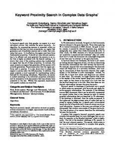
Another example uses data from the Internet Movie Database, or IMDB [15]. Figure 1 (shown in the Introduction) demonstrates how proximity graphs can reveal a community of actors from this dataset, with noticeable subcommunities: the Marx brothers, late 20th century film stars, and singers in movies from an earlier era. Figure 13 shows how drawing a proximity graph as a directed graph can reveal interesting temporal properties. A query connecting Doris Day with Halle Berry is displayed as a directed k-layered graph, where actors are placed as closer to one endpoint or another based on their proximity to those endpoints. Direction on the edges represents increasing distance from the source node (Day). Our measures are not only able to extract an interesting path from Day to Berry, but also are able to “layer” the intermediating actors showing temporal progression from one era to another. Doris [I] Day 1949

Figure 11: Proximity graph for computer scientists Rivest, Knuth, Shamir and Adelman from the DBLP co-authorship graph. The resultant graph shows other well-known colleagues, resulting in an interesting academic community. CFEC=1.30e+1. Subgraph captures 99.6% with minsize = 12.

6.0 Bob Hope 7851

7.0

20.0

7.0

Elizabeth Taylor (I) 6936

than 0.765. We show the difference between the two movies in a different way in Figure 12. This graph shows each movie with its 10 closest neighbors, and links between movies that have high proximity to each other. We see that not only does Barton Fink have lower proximity values to its neighbors, but that those neighbors also are not closely connected to each other, In fact, only two of its neighbors are close in proximity to each other. On the other hand, Speed’s neighbors are often closely related to each other, and make up an easily recognizable genre of tense action movies. In addition, this cluster has two subclusters - political intrigue thrillers (Air Force One, Murder at 1600, Executive Decision, etc.) and the rogue-cop-saves-the-day-again action movie subcluster (Die Hard 2, Lethal Weapon 2, Lethal Weapon 3).

17.0

Millers Crossing Barton Fink

Mean Streets

Down by Law Wild at Heart The Hudsucker Proxy

The Man Who Wasnt There

Murder at 1600

The Client

Michael Jackson (I) 2796

12.0

Barbra Streisand 3372

11.0

9.0 Madonna (I) 4065

8.0

Nicole Kidman 3839 10.0

Outbreak

In the Line of Fire

Halle Berry 4161

Figure 13: Proximity graph between Halle Berry and Doris Day showing the community connecting them as a directed graph. CFEC=4.97e-7. Subgraph captures 78.3% with minsize = 8, maxsize = 10.

Executive Decision

Air Force One

Speed

Frank Sinatra 7677

Drugstore Cowboy

Blood Simple

Mystery Train

13.0 8.0

8.0

7.0

Ed Wood

24.0

U.S. Marshals

Die Hard 2: Die Harder Lethal Weapon 2 Lethal Weapon 3

Figure 12: Proximity graph showing communities around Barton Fink and Speed for the Netflix data

7.4 Showing Proximities via Directed Graphs to Show Temporal Effects

7.5 Proximities For Dense Graphs: Making a Similarity Measure More Reliable by Sparsification The usual targets of the CFEC proximity measure are datasets associated with sparse similarity functions, which are readily modeled as weighted graphs. That is, we directly measure similarity for only a relatively small number of objects, and CFEC proximity measurement fills in the missing similarity values. Interestingly, a further application of CFEC proximity is for datasets with dense similarity measures, where we are given an explicit similarity value between many or all object pairs. Apparently, a network-based proximity measure such as CFEC should be superfluous, as all similarities are already given. However, often, we have confidence only in the highest similarities, whereas most of the given similarities are not considered reliable. One example is the bioPIXIE

dataset [21], where pairwise functional relationships between proteins were compiled by combining information from multiple heterogeneous sources. While some evidence for pairwise relationships can be found for almost any two proteins, substantial evidence for functional relationships exists for far fewer protein pairs. Consequently, it was suggested to use only the similarities for which we have high confidence. This way, relationships between protein pairs are defined by a network of reliable relationships. In such cases, when given a dense similarity measure, we would like to assess the competitiveness of the CFEC proximity measure– based on combining many reliable strong similarities– against a direct, but possibly less reliable similarity measure. (This is similar in spirit to local linear embedding algorithms such as Isomap [25], where geodesic distances, computed by summing multiple short, “reliable” distances, are preferred over direct distances.) Based on the above observations, we conducted a study with the Netflix dataset. This dataset enables us to evaluate the performance of the CFEC similarity measure from a unique perspective, by comparing how CFEC fares against direct similarities. Moreover, it suggests a new application for CFEC proximity, as a way of estimating values associated with nodes. The Netflix dataset was gathered by the online video rental firm Netflix, and published as part of a contest [22]. The goal of the contest is to accurately predict user ratings on movies. The dataset contains over 100 million ratings from 480,000 randomly-chosen, anonymous Netflix customers over 17,000 movie titles. Each rating is an integer between 1 to 5. We can directly measure the similarity between two movies as long as the two movies share ratings by the same users. Let us denote the common support of two movies i and j as N (i, j), which is the set of users that rated both movies. A suitable measure of distance would be the mean squared error (MSE) between the ratings of the two movies, defined as: P 2 u∈N(i,j) (ru (i) − ru (j)) MSE(i, j) = |N (i, j)| where ru (i) ∈ {1, . . . , 5} is the rating of movie i by user u. Certainly, as |N (i, j)| grows, the resulting MSE(i, j) is more reliable, because it is based on more information. In other words, a distance measured for two movies co-rated by 1000 users is more significant than if they were co-rated by only 100 users. Consequently, it is crucial to shrink the movie-movie distances towards the global mean as the size of their support set decreases. In practice, this way we can measure the similarity of almost any two movies. Similarity values directly lead to a rating prediction rule. Given a user u and a movie m such that we want to predict the corresponding rating ru (m), we can rely on all the movies rated by user u, denoted by N (u). The estimate would be: P i∈N(u) sim(m, i) · ru (i) P ru (m) ∼ (10) i∈N(u) sim(m, i)

where sim(m, i) is a non-negative similarity measure between the movies m and i. We measured the quality of the prediction rule with a Netflixsupplied probe dataset containing pairs for which we know the true ratings. We selected 100,000 representative pairs out of this probe dataset. Prediction quality is measured as the root mean squared error (RMSE) between the predicted and true ratings. Direct similarities can be taken as a decreasing function of the shrunk MSE values. Accordingly, we define sim(m, i) = exp(−MSE(m, i)). By applying the prediction rule (10), we predicted the scores for the 100,000 probe pairs with a resulting RMSE of 1.01.

Alternatively, we could rely on only the significant relations, those involving movie-pairs with low respecting shrunk MSE values, and then compute the similarity between movie pairs using our proximity measure. More specifically, our graph contained 17,770 nodes (corresponding to movies), and each movie was linked to its 50 most similar movies by an edge of weight exp(−MSE(m, i)). As before, we employed the prediction rule (10), but this time using the CFEC proximity function: sim(m, i) =CFEC(m, i). This yields better predictions, reflected by a lower RMSE of 0.975. For comparison, Cinematch, Netflix’ proprietary rating system, produced scores for a comparable dataset with RMSE of 0.951. It appears that replacing direct proximities with CFEC proximities goes a long way in reducing the RMSE towards the result of the well tuned Cinematch system, even before applying other potential improvements. Besides being an encouraging indication of the validity of the CFEC proximity measure, the Netflix dataset also provides a new application for network proximity measurement, which we hope to pursue further. There are some details concerning efficient implementation here. The average number of ratings per user is about 210. Thus, a naive calculation of prediction rule (10) based on CFEC proximity requires, on average, the computation of 210 CFEC proximities, which is excessively expensive. However, since we have at most 5 distinct rating values by a user, we can significantly speed up the computation by merging all movies that were rated equally by the same user. This way, when we need to estimate the rating of movie m by user u, we merge all nodes corresponding to movies rated 1 by u into a single super-node v1 ; similarly, all movies in {i|i ∈ N (u), ru (i) = α} are merged into a super-node vα for α = 1, . . . , 5. When merging nodes, weights of duplicated edges are accumulated. Thus, to estimate ru (m) we need to compute only 5 CFEC values, which are CFEC(m, v1 ), CFEC(m, v2 ), . . . , CFEC(m, v5 ) and prediction rule (10) becomes: P5 α=1 CFEC(m, vα ) · α ru (m) ∼ P 5 α=1 CFEC(m, vα )

As a result, we achieved an average computation time of 3 seconds per estimate on a 2.6GHz Pentium-4 PC.

8. CONCLUSIONS Networks are a ubiquitous data representation, motivating the search for good methods of measuring proximities among network objects. We found that obvious, simplistic approaches have limitations that make them inappropriate for many kinds of real life, adhoc networks. Consequently, we introduced a proximity measure based on the notion of cycle-free effective conductance (CFEC). CFEC proximity was shown to exhibit many desired characteristics. While no proximity measure can be suitable for all kinds of data, the methodical examination that led to the choice of CFEC proximity suggests that it will be useful for a wide range of networked data. In particular, we observed good results with several practical datasets. A proximity measure for networked objects can be much more useful in data analysis when accompanied by a way of explaining and demonstrating measured proximity values. CFEC proximity allows us to compute proximity graphs, which are small portions of the network that are aimed at capturing proximity values. A significant benefit is that an analyst studying relationships between nodes in a large network can focus on only small portions of a network that are relevant to the measured proximity. This is far more practical than displaying and manually exploring a network with thousands or even millions of nodes. Moreover, proximity

graphs are of interest beyond their application to explaining measured proximity values. They can be regarded as an extension of [13] “connection subgraphs” introduced by Faloutsos et al [10]. Connection subgraphs provide a compact representation of the relationships between two network objects. Proximity graphs can serve the same purpose, while explicitly capturing CFEC proximity. In this [14] application, proximity graphs have the advantages of showing relationships between more than two endpoints, accommodating paths in directed graphs, and efficient approximation by solving an opti[15] mization problem that has tunable parameters. [16] We experimented with four datasets that shared certain properties, such as apparent log-normal distribution of CFEC proximities, small-world phenomena, and the ability to extract proximities using small subgraphs. In the future, we would like to understand [17] what properties would make network datasets unsuitable for CFEC proximity. Also, we would like to study whether “natural” self[18] organizing networks tend to allow extracting proximity using relatively small subgraphs, as we observed experimentally. We invite the reader to explore a web site that demonstrates prox[19] imity graphs, at http://public.research.att.com/˜volinsky/ cgi-bin/prox/prox.pl. On this page the user can create [20] proximity graphs from the IMDB or DBLP databases. Queries take only a few seconds to execute, including generation of the candidate graph and and creating and rendering the proximity graph. The [21] user can also experiment with different values of the parameters α, minsize, and maxsize.

9.

REFERENCES

[1] A.-L. Barabasi and R. Albert. Emergence of scaling in random networks. Science, 286:509–512, October 1999. [2] R. M. Bell, Y. Koren, and C. Volinsky. Modeling relationships at multiple scales to improve accuracy of large recommender systems. In KDD ’07: Proceedings of the 12th ACM SIGKDD international conference on Knowledge discovery and data mining, 2007. [3] I. Bhattacharya and L. Getoor. Relational clustering for multi-type entity resolution. In Proc. 11th ACM SIGKDD Workshop on Multi Relational Data Mining, pages 3–11, 2005. [4] B. Bollobas. Modern Graph Theory. Springer-Verlag, 1998. [5] U. Brandes and D. Fleischer. Centrality measures based on current flow. In Proc. 22nd Symp. Theoretical Aspects of Computer Science (STACS ’05), pages 533–544. LNCS 3404, Springer-Verlag, 2005. [6] J. D. Cohen. Drawing graphs to convey proximity: an incremental arrangement method. ACM Transactions on Computer-Human Interaction, 4(3):197–229, 1997. [7] T. H. Cormen, C. L. Leiserson, and R. L. Rivest. Introduction to Algorithms. McGraw-Hill and the MIT Press, 1990. [8] DBLP computer science bibliography. dblp.uni-trier.de. [9] P. G. Doyle and J. L. Snell. Random Walks and Electrical Networks. The Mathematical Association of America, 1984. http://arxiv.org/abs/math.PR/0001057. [10] C. Faloutsos, K. S. McCurley, and A. Tomkins. Fast discovery of connection subgraphs. In Proc. 10th ACM SIGKDD Conference, pages 118–127, 2004. [11] G. Flake, S. Lawrence, and C. L. Giles. Efficient identification of web communities. In Proc. 6th Sixth ACM SIGKDD Conference, pages 150–160, Boston, MA, August 20–23 2000. [12] M. R. Garey and D. S. Johnson. Computers and Intractability, A Guide to the Theory of NP-Completeness.

[22] [23]

[24]

[25]

[26]

[27]

W.H. Freeman and Company, New York, 1979. D. Gibson, J. M. Kleinberg, and P. Raghavan. Inferring Web Communities from Link Topology. In Proceedings of the 9th ACM Conference on Hypertext and Hypermedia, pages 225–234, Pittsburgh, Pennsylvania, June 1998. E. Hadjiconstantinou and N. Christofides. An efficient implementation of an algorithm for finding k shortest simple paths. Networks, 34:88–101, 1999. Internet Movie Database. www.imdb.com. M. M. John Hershberger and S. Suri. Finding the k shortest simple paths: A new algorithm and its implementation. In Proc. 5th Workshop on Algorithm Engineering and Experimentation (ALENEX ’05), pages 26–36. SIAM, 2003. N. Katoh, T. Ibaraki, and H. Mine. An efficient algorithm for k shortest simple paths. Networks, 12:411–427, 1982. Y. Koren, S. C. North, and C. Volinsky. Measuring and extracting proximity in networks. In Proc. 12th ACM SIGKDD Conference, pages 245–255, 2006. K. Lang. Finding good nearly balanced cuts in power law graphs. Technical report, Yahoo Research Labs, 2004. D. Liben-Nowell and J. M. Kleinberg. The link prediction problem for social networks. In CIKM, pages 556–559. ACM, 2003. C. L. Myers, D. Robson, A. Wible, M. A. Hibbs, C. Chiriac, C. L. Theesfeld, K. Dolinski, and O. G. Troyanskaya. Discovery of biological networks from diverse functional genomic data. Genome Biology, 6:R114, 2005. Netflix prize. www.netflixprize.com. A. Popescul and L. H. Ungar. Statistical relational learning for link prediction. In Proc. Workshop on Learning Statistical Models from Relational Data (IJCAI ’03), 2003. R. Salakhutdinov, A. Mnih, and G. Hinton. Restricted Boltzmann machines for collaborative filtering. In Proceedings of the 24th International Conference on Machine Learning (ICML 2007), pages 791–798, 2007. J. B. Tenenbaum, V. de Silva, and J. C. Langford. A global geometric framework for nonlinear dimensionality reduction. Science, 290:2319–2323, 2000. H. Tong and C. Faloutsos. Center-piece subgraphs: problem definition and fast solutions. In Proc. 12th ACM SIGKDD Conference, pages 404–413, 2006. W. E. Winkler. The state of record linkage and current research problems. Technical report, Statistical Research Division, U.S. Bureau of the Census, 1999.