Extracting Evolving Pathologies via Spectral Clustering - Springer Link

Extracting Evolving Pathologies via Spectral Clustering Elena Bernardis, Kilian M. Pohl, and Christos Davatzikos Section of Biomedical Image Analysis, Department of Radiology, University of Pennsylvania, Philadelphia, PA 19104

Abstract. A bottleneck in the analysis of longitudinal MR scans with white matter brain lesions is the temporally consistent segmentation of the pathology. We identify pathologies in 3D+t(ime) within a spectral graph clustering framework. Our clustering approach simultaneously segments and tracks the evolving lesions by identifying characteristic image patterns at each time-point and voxel correspondences across time-points. For each 3D image, our method constructs a graph where weights between nodes capture the likeliness of two voxels belonging to the same region. Based on these weights, we then establish rough correspondences between graph nodes at different time-points along estimated pathology evolution directions. We combine the graphs by aligning the weights to a reference time-point, thus integrating temporal information across the 3D images, and formulate the 3D+t segmentation problem as a binary partitioning of this graph. The resulting segmentation is very robust to local intensity fluctuations and yields better results than segmentations generated for each time-point. Keywords: 4D segmentation, longitudinal tracking, MRI white matter lesion.

1 Introduction The diagnosis of white matter brain lesions often involves the analysis of longitudinal MR brain scans. This type of analysis can greatly benefit from accurately segmenting the lesions across the scans. However, the task is difficult to perform when done for each time-point individually as lesions are often hard to detect. They might appear very faint and white matter might be erroneously identified as lesions due to intensity fluctuations. These issues can be minimized by considering all time-points during segmentation, as lesions show up more clearly at later time-points and intensity fluctuations of white matter are not consistent across time-points. We propose an algorithm to extract 3D+t lesions by simultaneously capturing structural and temporal consistency in a spectralgraph framework. While several 3D+t methods for temporally consistent healthy tissue segmentation [7,13,5,8,15] and for 3D lesion extraction [12,6,11,1] have been proposed in the literature, few approaches have been explored to study longitudinal lesion changes [14,9]. An atlas of a healthy population is often relied upon both for the temporally consistent segmentation of healthy tissues of adult brains [8], as well as for 3D lesion segmentation, which generally flag lesions as outliers. These outliers are detected by first estimating intensity distributions for the pathology and then incorporating contextual information in the classification [12], computing spatial posterior probabilities of each tissue in a J.C. Gee et al. (Eds.): IPMI 2013, LNCS 7917, pp. 680–691, 2013. c Springer-Verlag Berlin Heidelberg 2013 

Extracting Evolving Pathologies via Spectral Clustering Affinities

Affinities

Affinities

4D segmentation

Contours

time T

time 2

time 1

3D+T images

681

Correspondences − Fig. 1. Method Overview. First, we construct pairwise affinities Q+ t and Qt for each 3D image It to capture the characteristic patterns of lesions vs. background. Second, we compute rough correspondences C between time-points by finding best affinities’ matches. Affinities are then aligned to the first-time point and combined into one affinity matrix W , which now carries both structural and temporal information. Finally, we use spectral clustering to find the final 3D+t partition X, which is then back-projected to each It .

Bayesian framework [6], or adding topological constraints in addition to the statistical atlases [11]. Alternatively, [1] uses k-nearest neighbors classification to generate a label map outlining lesions. Adapting these lesion segmentation methods to the temporal domain is not straightforward as not only the lesions have to be interpreted as abnormal tissue not captured by the atlas, but their appearance across time-points has also to be taken into account. Alternatively, extensions to integrate spatial and temporal information in 3D+t lesion models include characterizing lesions by building a spatiotemporal lesion evolution model [14], or capturing implicit lesion information at each voxel by first computing displacement fields between time-points and then clustering the evolving lesions based on vector field operators [9]. We propose a method that does not rely on comparisons to healthy tissue, and that seamlessly integrates the lesion segmentation and tracking steps into one principled approach. We base our approach on spectral clustering [10,16], which has the ability to grasp the structural organization of an image from the global integration of local cues. Spectral clustering has been successfully used for the automatic segmentation of small, round structures (e.g. epithelial cells or lymphocytes) in 2D microscopic images [3], and extended to extract tubular structures in 3D microscopic images [4]. Images are represented by a graph, where nodes in the graph correspond to voxels in the image.

682

E. Bernardis, K.M. Pohl, and C. Davatzikos

Weights associated to edges between graph nodes capture pair-wise affinities between voxels. Positive affinities indicate the likelihood of two voxels belonging to the same region while the opposite is true for negative affinities. By computing the top eigenvectors of this weight matrix, each voxel is represented by a point in the embedding space. The desired segmentation is obtained by straight-forward clustering of the voxels in this embedding space. Our spectral graph method extracts lesions from longitudinal MR scans by defining grouping cues that distinguish lesions from healthy tissue. Specifically, we first construct pairwise affinities from each 3D image to characterize brighter regions of varying shapes and sizes. We then reduce the complexity of the 3D+t segmentation task by transforming it into a 3D one. We do so by explicitly tracking the graph nodes across time-points. For each node, we estimate a possible evolution direction of the pathology. Correspondences between adjacent time-points are then found by best affinities matching of the nodes along this direction. We use these correspondences to align each graph to a reference time-point, so that weights can be combined into one graph. This new graph now captures both structural and temporal affinities between nodes. To the best of our knowledge, this way of enforcing temporal consistency is very different in nature from any temporal consistent segmentation approach in medical imaging. Our method is fully automatic and depends only on a few parameters. Additional time-points can be easily added to the graph as the method only requires computing the additional grouping cues at the new time-point as well as the projections to the previous one. Finally, our method is purely intensity-based and does not use any prior knowledge about the lesions other than that they are brighter than their background. While we test the approach only on longitudinal MR scans showing brain lesions, our method should be applicable to many other pathologies that full-fill these requirements.

2 Segmenting 3D+t Pathologies by Spectral Graph Partitioning We segment lesions from 3D+t MR via a spectral graph theoretic framework. We assume the scans of each time are pose-corrected, so that across time-points healthy tissue remains constant and only the evolving pathology is changing. An overview of our method is given in Fig. 1. For each time-point, we compute − pairwise voxel affinities, called attraction Q+ t and repulsion Qt , that capture differences between high and low intensity regions and whether two voxels might belong to a lesion region (Sec. 2.1). We then determine correspondences Ct between voxels at different time-points (Sec. 2.2) by tracking graph nodes. Given the correspondences, we map the affinities at each time-point to a reference to generate a new graph where weights now also carry temporal information (Sec. 2.3). The final 3D+t segmentation is found by partitioning this graph via spectral clustering (Sec. 2.4). 2.1 Creating a Graph for Each Time-Point: Computing Affinities in 3D We start by constructing the graph Gt (N, E, Wt ) at each time point t = 1, . . . T . Let It be the 3D scan associated with time-point t. Voxels of It are represented as nodes N in the graph and the N × N weight matrix Wt captures the affinity of the edges E

Extracting Evolving Pathologies via Spectral Clustering b: pairwise attractions between nodes and

a: image intensity

c: pairwise repulsions p between nodes and
  
  





Intensity Attraction
Mij

j2

683





 

j1

i

peak-valley-peak i

j1

j2

i

j1

j2

Intensity Attraction
M


  
  





ij

i





 

j1 j2

peak-peak-peak i

j1

j2

i

j1

j2

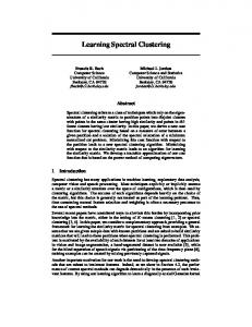
Fig. 2. Pairwise affinities. a: Image It with two neighboring nodes scenarios highlighted. In each case we plot, for j ∈ Nb (i), nodes at increasing radii of i along one direction b; b: intensities It (j) (blue), maximum intensity differences ΔMij (gray) and final pairwise attractions Q+ (i, j) (green). c: intensities Ij (blue) and final pairwise repulsions Q− (i, j) (red), computed as a func− tion of relative and absolute repulsion terms Q− rel (i, j) and Qabs (i, j) (both in gray). The absolute (gray star) is only direction dependent so it remains constant for all j ∈ Nb (i). minimum mabs i

between voxels. Affinities are composed of an attraction and a repulsion term, which we now define in further detail. Attraction Q+ t . Since lesions appear bright in Flair MR scans, attraction should be large between neighboring voxels with high and similar intensities. We measure this type of attraction between voxels (i, j) as a function of the maximum intensity difference ΔMij := maxs∈line(i,j) |It (i) − It (s)| attained along the 3D line(i, j) connecting them, where It (i) is the intensity at node i, and j is a node in i’s neighborhood N (i) = {j ∈ N (i)|d(i, j) ≤ ra } with attraction radius ra . We then define the pairwise attraction Q+ (i, j) between (i, j) as [2]:   2  1 ΔMij + Qt (i, j) := exp − 2 (1) σa δi where δi := | maxj∈N (i) Ij −minj∈N (i) Ij | is the intensity range of the entire neighborhood N (i) and σa is a fixed parameter. Figure 2b visualizes Q+ t (i, j) and ΔMij along one sample line as j moves away from i. ΔMij enforces a decreasing affinity once j has passed the node with maximum intensity difference from i. Furthermore, scaling ΔMij by the neighborhood intensity range δi at each node effectively normalizes the affinities within each neighborhood. This scaling has also the effect of enhancing weaker

684

E. Bernardis, K.M. Pohl, and C. Davatzikos

intensity regions, thus allowing to capture faint regions near a salient one, which can be easily missed. Repulsion Q− t . To extract brighter regions from the darker background, we add a repulsion term between background voxels and possible lesion ones. We denote high intensity regions by ‘peaks’ and low intensity regions by ‘valleys’. Let the neighborhood of i be N (i) = {j ∈ N (i)|d(i, j) ≤ rr } with repulsion radius rr . A simple definition of repulsion between nodes i, j could be defined by their intensity difference: Q− rel (i, j) := |It (j) − It (i)|.

(2)

Q− rel

would ignore the relative location of i and j with Setting repulsion solely on respect to the peaks and valleys. We thus need to estimate whether i, j lie both on the same peak, both on peaks but are separated by a valley, or one on a peak and the other in a valley (illustrated in Fig. 2a). We achieve this by determining the minimum intensity mrel ij := mins∈line(i,j) It (s) attained between i and j. We then measure for i and j the rel intensity difference to this minimum: Δmi := |It (i)−mrel ij | and Δmj := |It (j)−mij | respectively. When the intensity of i is closer to the minimum compared to that of j, i.e. Δmi = min(Δmi , Δmj ), then the node i is adjacent to a region of higher intensity (since all nodes j are at higher intensity - as in the case of node i in the second row of Fig. 2), so we do not want i to repel its neighbors j. On the other hand, if j’s intensity is closer, we then have the two possible scenarios illustrated in first row of Fig. 2 : peak(i)-valley(j1) or peak(i)-valley-peak(j2). In both cases, we want the repulsion term between i and j to capture the presence of the valley, i.e. a measure of the intensity drop attained between them. How much repulsion is added between these two nodes should depend on how much the intensity of node j differs from the absolute minimum := minj∈line(i,k) mrel intensity mabs i ij (gray star in Fig. 2c) attained along the entire line (i.e. k is the farthest node along that direction line). We thus define:  abs |mi − It (j)| if Δmj = min(Δmi , Δmj ) − Qabs (i, j) := (3) 1 otherwise. We can finally define the repulsion between nodes i, j as a function of Q− rel , weighted : by a function of Q− abs      − 2  2   − Q Q (i, j) (i, j) 1 abs rel 1 − exp − (4) Q− t (i, j) := exp − 2 σabs δ(i) σrel where σabs and σrel are fixed parameters and δi is again the intensity range of the − neighborhood N (i). Figure 2c illustrates how both Q− abs (i, j) and Qt (i, j) vary for nodes lying on the same line with two different intensity scenarios. In the top row, we have the configuration peak(i)-valley(j1) and peak(i)-valley-peak(j2). In the bottom row, all three nodes i, j1 , j2 belong to the same peak. The final repulsion Q− t (i, j) is highlighted in a red. The weights Wt at time-point t are then given by subtracting the repulsion Q− t from : the attraction Q+ t − Wt = Q+ (5) t − Qt . When repulsion is higher than the attraction between two nodes, the weights will have negative entries. This completes our definition of the graph Gt at time point t.

Extracting Evolving Pathologies via Spectral Clustering

685

2.2 Establishing Correspondences between Time-Points To combine the affinities computed at each time-point, we need to track the changes across the graphs G1 , . . . , GT . This is achieved in two steps. First, we compute the nodes’ correspondences Ct→t−1 from each time-point to the previous one. Then, we iteratively find the correspondences at each node to a reference time-point. We choose the first time-point as our reference for convenience since lesions only expand in time. We start by finding the correspondences Ct→t−1 to the previous time-point. Namely, for each for node i at time t, we find within the rc radius neighborhood of i the node j at time t − 1 whose affinities at t − 1 best match the affinities of i at time t. To achieve this, we reformat the weights Wt (i, :) of Eqn. 5 so that the affinities Wt (i, :) at i can be written as a 1 × J vector Wt (i, :), where J is the number of neighbors of i and entries in this vector correspond to the same neighborhood (relative) coordinates with respect to the center node i. Weights at each node are normalized by their outgoing  −1 ˜ t (i, :) = W  (i, :)[ . The correspondence of i to the connections, i.e. W t j Wt (i, j)] previous time-point is then defined by the voxel which minimizes the dot product d ˜ t: between the corresponding normalized weights W ˜ t (i, :), W ˜ t−1 (j, :)), Ct→t−1 (i) = argminj∈Ne (i) d(W

(6)

where we define the eligible neighbors Ne (i) ⊂ N (i) based on the evolving direction of the lesion. Given that the contour of the lesion are closed, we can think of the contours always evolving along the normal of the contour. We therefore compute this direction based on the affinities Wt at each time-point. Specifically, letting ix , iy , iz be the 3D spatial coordinates of voxel i corresponding to node i, we define at each node the evolution vector vt (i) ∈ R3 : ⎞ ⎛ jx − ix

vt (i) = Wt (i, j) ⎝jy − iy ⎠ . (7) jz − iz j∈N (i) For nodes near lesions, vt will always point towards the center of the nearest highest intensity area, i.e. towards the interior of the lesion at that time-point. Ne (i) could be defined by nodes along vt (i) (for regions expanding from t − 1 to t) or in the opposite direction −vt (i) (for regions contracting from t − 1 to t). Since lesions only expand in time, we restrict Ne (i) to nodes in direction vt (i). Fig. 3a, shows sample vectors vt . Finally, we determine the correspondences at each node to the first time-point, setting C1 (i) = i, by iterating the following recursion: Ct→1 (i) = Ct−1→1 (Ct→t−1 (i)).

(8)

2.3 Graph Setup across Time-Points: Aligning Affinities Once the correspondences Ct→1 have been computed, we can align the attraction and − repulsion cues Q+ t (i, j) and Qt (i, j) computed in Sec. 2.1 to obtain the aligned graphs Gt→1 (N, E, Wt→1 ). We compute the aligned attraction and repulsion, denoted by Q+ t→1 and Q− t→1 , separately to keep track of each cue’s influence. For simplicity, we let Ct (i) = Ct→1 (i) in the remainder of this section.

686

E. Bernardis, K.M. Pohl, and C. Davatzikos a: evolution vectors

b: original affinities

c: aligned affinities

region at time t

region at time 1

Fig. 3. Tracking temporal changes. a: Image It and evolution vector vt at each node. Vectors for nodes n1 , n2 , n3 are highlighted in yellow. For these nodes, we also illustrate on It , the corresponding node nk at t = 1 (region boundary at It=1 traced in green); b: attraction Q+ t and + − for n , n , n , n ; c: aligned attraction Q and repulsion Q at n . repulsion Q− 1 2 3 k k t t→t−1 t→t−1

One outstanding issue is what happens if multiple nodes at time t point to the same point at time 1, as well as those points at time 1 that have no correspondence at time t . We solve this issue by averaging as well as interpolating. For each node i that shifts to a new position k, i.e. Ct (i) = k and k = i, we find all other nodes S that also shift to that location, i.e. S = {s ∈ S|C(s) = k}. A sample scenario is depicted in Fig. 3a. For each one, we obtain the aligned cues at the new node k by averaging the ones from the originating nodes (see Fig. 3b-c): Q± t→1 (Ct (i), :) =

1 |i ∪ S|



Q± t (s, :).

(9)

s∈{i∪S}

For the remaining nodes, i.e. fixed nodes with Ct (i) = i such that no other node maps to i (i.e. there are no other nodes s such that Ct (s) = i), we simply leave the affinities ± unchanged: Q± t→1 (i, :) = Qt (i, :). The cues can then be collapsed into one graph by normalizing attraction and repulsion separately and then combining them to obtain the final cues: Q± =

T

t=1

−1 Q± t→1 DQ+

t→1

−1 + DQ Q± + t→1

(10)

t→1

where DQ is a diagonal matrix with entries D(i, i) = j Q(i, j). We normalize each cue separately, to keep track of how they factor in at each node. The final weight matrix W = Q+ − Q− contains pairwise affinities between nodes that capture both structural and temporal information between them. 2.4 Graph Segmentation via Spectral Clustering We will now find the 3D+t segmentation X of our images by applying spectral partitioning on the constructed graph G(N, E, W ).

Extracting Evolving Pathologies via Spectral Clustering

687

Spectral clustering is based on the following grouping criterion [16]: max ε =

within-group attraction between-group repulsion + total degree of attraction total degree of repulsion

(11)

Let the partition X of graph G be represented as a N × k binary matrix, so that X(i, g) equals 1 if node i belongs to group g. The criterion can be then formulated in the following matrix form: maximize

ε(X) =

k

XgT W Xg

XgT DXg

(12)

X ∈ {0, 1}N ×k , X1k = 1N

(13)

g=1

subject to

where 1N denotes the N × 1 vector of 1’s , and the weights are normalized by D, the diagonal matrix containing the degrees of W = Q+ − Q− , thus D(i, i) = j Q+ (i, j) − Q− (i, j). As was shown in the original framework [10], normalizing each node by its outgoing connections adds a sense of group balance. A near-global optimal solution can be computed by solving for the top k eigenvectors of the normalized matrix W [16]. Since we are seeking only a binary segmentation, the final voxel labeling can be obtained by simply thresholding the top second eigenvector (thus needing only k = 2). The 3D+t segmentation mask can finally be displayed on each individual 3D image It by back-tracking the nodes to obtain the segmentations X1→t at each It .

3 Experiments We apply our method to extract white matter lesions from longitudinal MR brain scans. We start by describing our data and provide implementation details for our method. We then illustrate results on 4D images and compare them to individual 3D segmentations. Baseline and follow-up scans were acquired on 1.5-Tesla scanners, with a 36 months interval for the follow-ups. All modalities have been rigidly registered to T1 using FSLs Flirt tool. For the first group, images belong to subjects with diabetes-2 and T = 2 timepoints. The T1 images are skull-stripped using an automated tool and the brain masks are then manually corrected. For the second group, images belong to healthy subjects and lesions are due to normal aging, T = 3 and skull-stripping is not applied a priori. For all our experiments, we only use Flair image modalities so lesions always appear as higher intensity regions embedded within the brain’s white matter. By definition, white matter lesions lie solely within the white matter of the brain and, in Flair images, always have higher intensity than the average intensity of the brain. We observe that the darker regions, such as cerebrospinal fluid (CSF) and ventricles, on the other hand always have intensities lower than the average. To create stronger attraction and repulsion cues between regions, we ‘invert’ the darker regions by taking It = |It − mean(It )| at each time-point. We therefore seek to extract lesions, CSF and

688

E. Bernardis, K.M. Pohl, and C. Davatzikos b: 3D output

c: 3D+t results

a: image t=2

b: 3D output

c: 3D+t results

appearing

enhancing

false positive

refining

a: image t=1

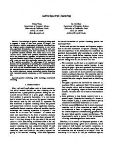
Fig. 4. 3D+t versus 3D segmentation. a: input It for 2 time-points; b: contours extracted from 3D segmentation Xt ; c: contours extracted from our final 3D+t segmentation X1→t . Both timepoints benefit from each other. In each row, we illustrate different scenarios in which 3D+t improves over 3D by: (i) refining contours; ii) eliminating false-positives (i.e. lesions that disappear in time); (iii) enhancing fainter regions and segmenting regions that would otherwise not be detected, which includes (iv) enhancing at earlier time-points lesions that will appear at later times.

ventricles from their common white matter background. Once a segmentation is found for this new image, we simply threshold out regions below the original intensity average to obtain the final lesions. We then apply our new graph construction to the It images. To compute affinities and correspondences, we adopt 3D neighborhoods N (i) = {j ∈ N (i)|d(i, j) ≤ r and directions b = (θ, φ)} with radii rr = 30 and ra = rc = 10 for repulsion, attraction and correspondences respectively. Neighbors are computed along spherical coordinate directions [θ = 0, φ = {0, ±π/4, ±π/2, ±3π/4, π}], [θ = ±π/2, φ = ±π/4], [θ = 0, φ = {±π/4, ±π/2, ±3π/4}]. We set σa = σrel = 0.3 and σabs = 0.5. Parameters are fixed for all images. We apply spectral clustering as described in Sec. 2.4, on the combined weight matrix W = Q+ −Q− and use the online code provided by [16] to solve for the final segmentation X. Running time for clustering the final graph G with W = Q+ − Q− is approximately 150 seconds for initial image sizes [128, 128, 30]. Figures 5 and 6 show 4D segmentation results for two different subjects, with T = 2 and T = 3 time-points respectively. For each X1→t , we visualize the contours extracted from the final 4D segmentation binary masks.

Extracting Evolving Pathologies via Spectral Clustering t=1

t=2

t=1

t=2

t=1

z=1

z=2

z=3

z=4

z=5

z=66

689 t=2

Fig. 5. Our 3D+t segmentation results for T = 2 time-points. Input images It together with final lesion contours extracted from X1→t at each time-point are shown for increasing z’s. For better visualization, disconnected lesions in 3D are illustrated with different colors.

We compare our results with the individual 3D segmentations by applying spectral − clustering directly on the individual weights Wt = Q+ t − Qt at each time-point t given by Eqn. 5. As illustrated for one subject in Fig. 4, advantages of 3D+t include: i) enhancing and/or detecting fainter regions at one time-point that appear more salient an another time; ii) refining boundaries; iii) eliminating false-positives, i.e. brighter regions due only to local intensity fluctuations at an earlier time-point that do not appear at later time-points. Clearly, if there is a consistent noisy region throughout all the time-points, the method would not be able to tell the difference. Note that appearing lesions are a special case of scenario (i): if a lesion appears at time t for the first time, all points on the contour of this new lesion will end up being matched to a single point at t − 1, corresponding to the center of the lesion at time t, thus defining an artificial ‘seed’ at t − 1. The appearing lesion will be properly detected at t and later time-points even if not present at the earlier ones. Alternatively, the lesion might be additionally enhanced if some faint region is already present but not sufficiently salient for a 3D segmentation to pick it up. As shown in Fig. 4, enforcing temporal consistency allows both earlier and later time-points to benefit from each other.

690

E. Bernardis, K.M. Pohl, and C. Davatzikos

t=1

t=2

t=1

t=3

z=1

z=2

z=3

z=4

z=5

z=6

t=2

t=3

Fig. 6. Our 3D+t segmentation results for T = 2 time-points. Input images It together with final lesion contours extracted from X1→t at each time-point are shown for increasing z’s. For better visualization, disconnected lesions in 3D are illustrated with different colors.

4 Conclusions We segment evolving pathologies via spectral graph clustering. At each time-point, we construct affinities that properly capture structural agreement and yield good segmentations, even when used in isolation for 3D segmentation. Across time-points, we track nodes that lie within an estimated pathology evolution direction by finding best matches of node affinities. The computed correspondences are used to align and combine affinities across time-points. Our method relies on two assumptions: regions of interest have higher intensities than their common background (for affinities computations), and 3D images are linearly registered (for node tracking). While we applied the method only to expanding lesions, expansion of the regions of interest is not required. Thanks to our graph construction, our final 3D+t segmentation has the same complexity as the 3D segmentations at each time-point. The method is scalable in time, as adding an additional time-point only requires computing the affinities and correspondences for the new image, and adding the aligned information to the already existing aligned graph from the other images for the final clustering step. As shown in our ex-

Extracting Evolving Pathologies via Spectral Clustering

691

periments, adding temporal information to segment the lesion allows all time-points to benefit from each other. Finally, while we used the correspondences only to enforce temporal consistency in the segmentation, they could also be used in future work to explicitly analyze the temporal shape changes of the extracted pathologies. Acknowledgments. This project was supported in part by the Institute for Translational Medicine and Therapeutics’ (ITMAT) and in part by NIH Grants UL1RR024134 and 5R01EB009234.

References 1. Anbeek, P., Vincken, K., Viergever, M.: Automated ms-lesion segmentation by k-nearest neighbor classification. In: Med. Image Comput. Comput. Assist. Interv. (July 2008) 2. Bernardis, E., Yu, S.X.: Robust segmentation by cutting across a stack of gamma transformed images. In: Cremers, D., Boykov, Y., Blake, A., Schmidt, F.R. (eds.) EMMCVPR 2009. LNCS, vol. 5681, pp. 249–260. Springer, Heidelberg (2009) 3. Bernardis, E., Yu, S.X.: Pop out many small structures from a very large microscopic image. Medical Image Analysis 15(5), 690–707 (2011) 4. Fragkiadaki, K., Zhang, W., Shi, J., Bernardis, E.: Structural-flow trajectories for unravelling 3D tubular bundles. In: Ayache, N., Delingette, H., Golland, P., Mori, K. (eds.) MICCAI 2012, Part III. LNCS, vol. 7512, pp. 631–638. Springer, Heidelberg (2012) 5. Habas, P., Kim, K., Corbett-Detig, J., Rousseau, F., Glenn, O., Barkovich, A., Studholme, C.: A spatiotemporal atlas of MR intensity, tissue probability and shape of the fetal brain with application to segmentation. NeuroImage 53(2), 460–470 (2010) 6. Prastawa, M., Gerig, G.: Automatic ms lesion segmentation by outlier detection and information theoretic region partitioning. In: Med. Image Comput. Comput. Assist. Interv. (September 2008) 7. Prastawa, M., Gilmore, J., Lin, W., Gerig, G.: Automatic segmentation of MR images of the developing newborn brain. Medical Image Analysis 9(5), 457–466 (2005) 8. Reuter, M., Fischl, B.: Avoiding asymmetry-induced bias in longitudinal image processing. NeuroImage 57(1), 19–21 (2011) 9. Rey, D., Subsol, G., Delingette, H., Ayache, N.: Automatic detection and segmentation of evolving processes in 3D medical images: Application to multiple sclerosis. Medical Image Analysis 6(2), 163–179 (2002) 10. Shi, J., Malik, J.: Normalized cuts and image segmentation. IEEE Trans. Pattern Analysis Machine Intelligence 22(8), 888–905 (2000) 11. Shiee, N., Bazin, P., Pham, D.: Multiple sclerosis lesion segmentation using statistical and topological atlases. In: Med. Image Comput. Comput. Assist. Interv. (October 2008) 12. Van Leemput, K., Maes, F., Vandermeulen, D., Colchester, A., Suetens, P.: Automated segmentation of multiple sclerosis lesions by model outlier detection. IEEE Transactions on Medical Imaging 20(8), 677–688 (2001) 13. Weisenfeld, N., Warfield, S.: Automatic segmentation of newborn brain MRI. NeuroImage 47(2), 564–572 (2009) 14. Welti, D., Gerig, G., Rad¨u, E.-W., Kappos, L., Sz´ekely, G.: Spatio-temporal segmentation of active multiple sclerosis lesions in serial MRI data. In: Insana, M.F., Leahy, R.M. (eds.) IPMI 2001. LNCS, vol. 2082, pp. 438–445. Springer, Heidelberg (2001) 15. Xue, Z., Shen, D., Davatzikos, C.: CLASSIC: Consistent longitudinal alignment and segmentation for serial image computing. NeuroImage 30(2), 388–399 (2006) 16. Yu, S.X., Shi, J.: Understanding popout through repulsion. In: IEEE Proc. Computer Vision and Pattern Recognition, pp. 752–757 (2001)