IEEE TRANSACTIONS ON INFORMATION THEORY, VOL. 50, NO. 11, NOVEMBER 2004
2657
Extrinsic Information Transfer Functions: Model and Erasure Channel Properties Alexei Ashikhmin, Member, IEEE, Gerhard Kramer, Member, IEEE, and Stephan ten Brink, Member, IEEE
Abstract—Extrinsic information transfer (EXIT) charts are a tool for predicting the convergence behavior of iterative processors for a variety of communication problems. A model is introduced that applies to decoding problems, including the iterative decoding of parallel concatenated (turbo) codes, serially concatenated codes, low-density parity-check (LDPC) codes, and repeat–accumulate (RA) codes. EXIT functions are defined using the model, and several properties of such functions are proved for erasure channels. One property expresses the area under an EXIT function in terms of a conditional entropy. A useful consequence of this result is that the design of capacity-approaching codes reduces to a curve-fitting problem for all the aforementioned codes. A second property relates the EXIT function of a code to its Helleseth–Kløve–Levenshtein information functions, and thereby to the support weights of its subcodes. The relation is via a refinement of information functions called split information functions, and via a refinement of support weights called split support weights. Split information functions are used to prove a third property that relates the EXIT function of a linear code to the EXIT function of its dual. Index Terms—Concatenated codes, duality, error-correction coding, iterative decoding, mutual information.
I. INTRODUCTION
T
HE seminal paper of Gallager [1, p. 48] suggested to evaluate the convergence behavior of iterative decoders for low-density parity-check (LDPC) codes by tracking the probability distributions of extrinsic log-likelihood ratios ( -values). The procedure is particularly simple for erasure channels (ECs) because one must compute only the fraction of erasures being passed from one component decoder to another. For example, this is done in [2], [3] for irregular LDPC codes. However, for other channels, one must track entire probability density functions. A detailed analysis for such cases is described in [4], [5], where the procedure is called density evolution. Density evolution can be simplified in several ways. First, empirical evidence shows that good EC codes are also good for many practical channels. This motivates designing codes for ECs, and then adapting the design for the actual channel [6,
Manuscript received March 25, 2003; revised March 15, 2004. The material in this paper was presented in part at the Conference on Information Sciences and Systems, Princeton University, Princeton, NJ, March 2002; the IEEE International Symposium on Information Theory, Lausanne, Switzerland, June/July 2002; and the 3rd International Symposium on Turbo Codes, Brest, France, September 2003. A. Ashikhmin and G. Kramer are with Bell Laboratories, Lucent Technologies, Murray Hill, NJ 07974 USA (e-mail:
[email protected];
[email protected]). S. ten Brink was with Bell Laboratories, Lucent Technologies, Crawford Hill, NJ. He is now with Realtek, Irvine, CA 92618 USA (e-mail: stenbrink@ realtek-us.com). Communicated by S. Litsyn, Associate Editor for Coding Theory. Digital Object Identifier 10.1109/TIT.2004.836693
Ch. 6]. A second approach is to track only one number per iteration rather than density functions. For instance, one might track a statistic of the extrinsic -values based on their mean, variance, an error probability, a fidelity or a mutual information [7]–[17]. We refer to [13, Sec. IV] and [18] for a comparison of some of these tools. We consider tracking a per-letter average mutual information, i.e., we use extrinsic information transfer (EXIT) charts. Several reasons for choosing EXIT charts are as follows. • Mutual information seems to be the most accurate statistic [13, Sec. IV], [18]. • Mutual information is the most robust statistic, in the sense that it applies without change to the widest range of channels, modulations, and detectors. For instance, EXIT functions apply to ECs without change. They further apply to symbol-based decoders [19] and to suboptimal decoders such as hard-decision decoders. • EXIT functions have analytic properties that have useful implications for designing codes and iterative processors. One aim of this paper is to justify the last claim. For example, we prove that if the decoder’s a priori -values come from a binary EC (or BEC) then the area under an EXIT function is one minus a conditional entropy. This property is used to show that code design for BECs reduces to a curve-fitting problem for several classes of codes including parallel concatenated (PC or turbo) [20], serially concatenated (SC) [21], LDPC, and repeat–accumulate (RA) codes [22], [23]. This fact gives theoretical support for the curve-fitting techniques already being applied in the communications literature, see, e.g., [24]–[30]. The success of these techniques relies on the robustness of EXIT charts: the transfer functions change little when BEC a priori -values are replaced by, e.g., a priori -values generated by transmitting binary phase-shift keying (BPSK) symbols over an additive white Gaussian noise (AWGN) channel. Moreover, the resulting transfer functions continue to predict the convergence behavior of iterative decoders rather accurately. For the special case of LDPC codes, the area property is related to the flatness condition of [31] and has similar implications. For both LDPC and RA codes on a BEC, the curve-fitting technique is known through a polynomial equation [2], [23]. However, the area property applies to many communication problems beyond LDPC or RA decoding. For instance, it applies to problems with PC codes, SC codes, modulators, detectors, and channels with memory. A second property we prove is that EXIT functions for BECs can be expressed in terms of what we call split information functions and split support weights. The former are refinements of the information functions of a code introduced in [32], while
0018-9448/04$20.00 © 2004 IEEE
2658
IEEE TRANSACTIONS ON INFORMATION THEORY, VOL. 50, NO. 11, NOVEMBER 2004
the latter are refinements of the weight enumerators of a code [33]–[35]. The split information functions are used to prove a third property that relates the EXIT function of a linear code to the EXIT function of its dual. As far as we know, these are the first applications of information functions and support weights to a posteriori probability (APP) decoding. This paper is organized as follows. The first part of the paper, comprising Sections II and III, deals with general channels. In Section II, we describe a decoding model that can be used for a wide variety of communication problems. In Section III, we use this model to define EXIT functions and derive general properties of such functions. The second part of the paper deals with BECs. In Section IV, we derive several properties of EXIT functions when the a priori -values are modeled as coming from a BEC. Sections V–VIII show how the area property guides code design. Section IX summarizes our results. II. PRELIMINARIES A. EXIT Chart Example Consider the EXIT chart for an LDPC code. Such a code is often represented by a bipartite graph whose left vertices are called variable nodes and whose right vertices are called check nodes (see [4]). Suppose the variable and check nodes have -regular degrees and , respectively, so that we have a and, as is often LDPC code. The code has a design rate of done, we assume the code is long and its interleaver has large girth. Suppose we transmit over a BEC with erasure probability . A belief-propagation decoder then passes only one of three proband (erasure). As we will show, the EXIT abilities: functions turn out to be one minus the fraction of erasures being passed from one side of the graph to the other, i.e., the analysis is equivalent to that of [2]. Fig. 1 shows the EXIT functions and . The curve for the check nodes is when the one starting at on the axis, and its functional form is . The curve for the variable nodes depends on and is given by . The decoding trajectories are depicted in Fig. 1 by the dashed , we begin lines marked with arrows. For instance, when axis at and move right to the check-node on the curve. We then move up to the variable-node curve marked , back to the check-node curve, and so forth. The curve does not intersect the check-node curve, which means the decoder’s per-edge erasure probability can be made to approach zero. We say that there is an open convergence tunnel between curve intersects the checkthe curves. In contrast, the node curve, which means the decoder gets “stuck.” Convergence , and is therefore called is, in fact, guaranteed if a threshold for this decoder. B. Decoding Model Consider the decoding model shown in Fig. 2. A binary-symmetric source produces a vector of independent information bits each taking on the values and with probability . An encoder maps to a binary length codeword . We write random variables using upper case letters and their realizations
Fig. 1. EXIT chart for a (2; 4)-regular LDPC code on the BEC.
Fig. 2.
A decoding model for PC and SC codes.
by the corresponding lower case letters. For example, we consider to be a realization of . The decoder receives two vectors: a noisy version of and a noisy version of , where is either or . We call the to channel the commuthe extrinsic nication channel, and the to channel channel. One might alternatively choose to call the extrinsic channel the a priori channel because we use its outputs as if they were a priori information. However, we will consider iterative decoding where this channel models extrinsic information [36] coming from another decoder rather than true a priori information. Either way, the terminology “extrinsic” reminds us that originates from outside the communication channel. that Fig. 2 depicts how we will model the information the component decoders of a PC or SC code receive. For example, suppose we perform iterative decoding for an SC code. The inner decoder receives extrinsic information about the input . The outer encoder, in bits of the inner encoder, so we set contrast, receives extrinsic information about the output bits of . In both cases, the extrinsic the outer encoder, so we set channel is an artificial device that does not exist. We introduce it only to help us analyze the decoder’s operation. Often both the communication and extrinsic channels are memoryless, but we remark that the area property derived below remains valid when the communication channel has memory. For example, suppose we parse the bits into 4-bit blocks, and map each of these blocks to a 16 quadrature amplitude modulation (16-QAM) symbol. We send these symbols through an AWGN channel and they arrive at the receiver as . We view the communication channel as including the parser,
ASHIKHMIN et al.: EXTRINSIC INFORMATION TRANSFER FUNCTIONS
Fig. 3.
2659
of the bits in . The appropriate model is then Fig. 3 (or Fig. 2) and an extrinsic channel that is absent or completely with noisy. for the vector with the For further analysis, we write th entry removed, i.e., . We expand the numerator in (3) as
A decoding model with two encoders.
the 16-QAM mapper, and the AWGN channel. This channel has a 4-bit “block memory” but the area property applies. (Of course, for such channels the property’s applicability to iterative decoding is hampered by the fact that the extrinsic channels are not accurately modeled as BECs.) As a second example, suppose we map onto BPSK symbols that are sent over an intersymbol interference (ISI) channel. The communication channel now consists of the BPSK mapper and the ISI channel. We will write for the capacity of the communication channel. Fig. 3 depicts another decoding model with two encoders. In fact, Fig. 3 includes Fig. 2: let Encoder 1 be the Encoder in choose Encoder 2 to be the identity mapping, Fig. 2, and if choose Encoder 2 to be Encoder 1. The reason and if for introducing the second encoder is that, when dealing with LDPC or RA codes, we need to make Encoder 1 the identity mapping and Encoder 2 a repetition code or single parity-check code. This situation is not included in Fig. 2. and An even more general approach is to replace with a combined channel . Such a model could be useful for analyzing the effect of dependencies between the channel and a priori -values. For other problems, the vector might have complex entries and Encoder 1 might be a discrete-time linear filter. We will, however, consider only the model of Fig. 3. Let be the length of , , , and . The decoder uses and to compute two estimates of : the a posteriori -values and , gives the extrinsic -values . The symbol , a priori information about the random variable with -value (1) is the probability that conwhere . Similarly, for memoryless comditioned on the event munication channels, the symbol gives information about the with -value random variable (2) We will use (2) when dealing with PC codes in Section VIII. For simplicity, we assume that all random variables are discrete. Continuous random variables can be treated by replacing certain probabilities by probability density functions. The decoder we are mainly interested in is the APP decoder [1] that computes the -values
(4) where and are vectors corresponding to , and where the last step follows if the extrinsic channel is memoryless. Expanding the denominator of (3) in the same way and inserting the result into (3), we have (5) where
(6) The value
is called the extrinsic -value about
.
III. EXIT FUNCTIONS A. Average Extrinsic Information An iterative decoder has two or more component decoders that exchange extrinsic -values. Alternatively, the decoders could exchange extrinsic probabilities. The ensuing analysis does not depend on how the reliabilities are represented because we use mutual information. Continuing, the from one decoder pass through an interleaver and are fed to another decoder as a priori -values . We model as being output from a channel as in Fig. 3. We define two quantities (see also [13]–[16]), namely (7)
(3)
(8)
where is the probability of the event conditioned on and . For example, suppose we perform a maximum a posteriori probability (MAP) decoding
As done here, we adopt the notation of [37, Ch. 2] for mutual information and entropies. The value is called the average is called a priori information going into the decoder, and
2660
IEEE TRANSACTIONS ON INFORMATION THEORY, VOL. 50, NO. 11, NOVEMBER 2004
the average extrinsic information coming out of the decoder. as a function of . An EXIT chart plots all have the same disConsider first , and suppose the tribution, and that the extrinsic channel is memoryless and time invariant. We then have (9) We further have because is binary. We will usually consider codes for which the are uniform and identically can distributed, and codes and extrinsic channels for which take on all values between and . Consider next . Observe from (6) that is a function of , and that and are interchangeable since one and defines the other. This implies (see [38, Sec. 2.10]) (10) rather than simply because better We will use reminds us of the word a priori. Some authors prefer to add , and similarly for entropies commas and write with multiple random variables. However, we will adhere to the notation of [37]. The following proposition shows that the inequality in (10) is in fact an equality for APP decoders with extrinsic message passing.
Fig. 4. EXIT chart for repetition codes on BECs (upper three solid lines), a BSC (lower solid line), and BPSK on an AWGN channel (dashed line).
extrinsic channels are binary-symmetric channels (BSCs) with crossover probabilities and , respectively. We now have
Proposition 1: (11)
where
Proof: See Appendix A. We remark that for non-APP decoders, the average extrinsic information put out by the decoder will usually not satisfy (10) with equality. The import of Proposition 1 is that we need to consider only random variables in front of the decoder, i.e., we have
is the binary entropy function. For the case we use (12) to compute
and
(12) (14) B. Examples Example 1: (Repetition Codes on a BEC) Consider Fig. 2 with a length repetition code. Suppose the communication and extrinsic channels are BECs with erasure probabilities and , . Furthermore, respectively. We have we have for the case
(13) where the second step follows by the symmetry of the code. We versus in Fig. 4 where we have chosen and plot . Example 2: (Repetition Code on a BSC) Consider the repetition codes of Example 1, but where the communication and
Similar curves can be computed for . We plot in Fig. 4 for with (it is the lowest solid curve). We , i.e., is approximately thus have the same as in Example 2. Observe that the BSC curve is close to but below the BEC curve. Similar observations concerning thresholds were made in [6, Chs. 6 and 7]. Example 3: (Repetition Code on an AWGN Channel) Consider the repetition codes of Example 1, but where the communication and extrinsic channels are BPSK-input AWGN chanand , respectively. We convert nels with noise variances these variances to the variances of their -values [36], namely, and , respectively. One can compute and , where
(15)
ASHIKHMIN et al.: EXTRINSIC INFORMATION TRANSFER FUNCTIONS
2661
We plot
in Fig. 4 for as the dashed curve, where so that . Observe that the AWGN curve lies between the BEC and BSC curves. Again, a similar result concerning thresholds was found in [6, Chs. 6 and 7]. In fact, recent work has shown that the BEC and BSC curves give upper and lower bounds, respectively, on the EXIT curves for repetition codes on binary-input, symmetric channels [39], [40].
Example 4: Consider LDPC variable nodes of degree . We , and Encoder use the model of Fig. 3 where is one bit, 2 is a length repetition code. We again make the communication and extrinsic channels BECs with erasure probabilities and , respectively. We compute
(16) Fig. 1 shows two examples of such curves when .
and
Example 5: Consider LDPC check nodes of degree . We and with Encoder 2 a length use the model of Fig. 3 with single parity-check code. Let the extrinsic channel be a BEC and (12) simplifies with erasure probability so that to
Example 7: (Irregular LDPC Codes) An irregular LDPC code [2] can be viewed as follows: Encoder 2 in Fig. 3 is a mixture of either repetition codes or single parity-check codes. For example, suppose that 40% and 60% of the edges are connected to degree- and degree- variables nodes, respectively. and , we have Inserting (16) into (19) with (20) are here the same as the left degree distribution coeffiThe of [2]. cients IV. ERASURE CHANNEL PROPERTIES The rest of this paper is concerned with the special case where the a priori symbols are modeled as coming from a BEC with erasure probability . We derive three results for EXIT functions for such situations. The first, an area property, is valid for any codes and communication channels. The second, an equation showing how to compute EXIT functions via the Helleseth–Kløve–Levenshtein information functions of a code [32], is valid when both the communication and extrinsic channels are BECs. The third, a duality property, relates the EXIT functions of a linear code and its dual. A. Area Property
(17) An example of such a curve with
We have
is plotted in Fig. 1.
Example 6: Consider Example 4 but where has bits single parity-check code. and Encoder 2 is a length is thus a systematic code. We The code with codewords compute
(18) We will use (18) for generalized LDPC codes in Section VII-A.
(21) where (22)
Let be the area under the EXIT function. We have the following result. Theorem 1: If the extrinsic channel (i.e., a priori channel) is a BEC, then for any codes (linear or not) and any communication channel (memoryless or not) we have
C. Mixtures of Codes Suppose we split into several vectors , , and encode each separately. Let and be those portions of the respective and corresponding to , and denote the length of by . Equation (8) simplifies to
(23) Proof: See Appendix B. Note that
(19)
and are the th entries of and , respectively, , and is the expression in square brackets in (19). is simply the average extrinsic information for Observe that is the average component code . Thus, the EXIT function of the component EXIT functions . This mixing property is known and was used in [24]–[28] to improve codes. where
which implies . We will consider prifor all so that . marily cases where For instance, suppose that Encoder 2 is linear and has no idle components, i.e., Encoder 2’s generator matrix has no all-zeros for all so that (23) becomes columns. This implies (24)
2662
IEEE TRANSACTIONS ON INFORMATION THEORY, VOL. 50, NO. 11, NOVEMBER 2004
TABLE I EXIT FUNCTIONS FOR SYSTEMATIC LINEAR BLOCK CODES
Furthermore, if both Encoders 1 and 2 are one-to-one (invertible) mappings then we can interchange , , and . For example, we can write (24) as (25) An important consequence of Theorem 1 is that it restricts the form of the EXIT function. Moreover, one can sometimes relate to the code rate, as shown in several examples below. We remark that we will use two definitions of rate interand . In most cases, these changeably: two rates are identical, but if Encoder 2 is not a one-to-one mapping then the second rate is smaller than the first. We will . ignore this subtlety and assume that Example 8: (Scramblers) Suppose Encoder 1 in Fig. 3 is a filter or scrambler, i.e., it is a rate one code. Suppose further that Encoder 2 is the identity mapping and the communication channel is memoryless. We then have and so that (25) gives (26) The area is therefore if independent and uniformly distributed binary inputs maximize (26). This result was discovered in [41] and motivated Theorem 1. Example 9: (No Communication Channel) Suppose there is no communication channel. Such a situation occurs for the outer . The area decoder of an SC code for which we also have (24) is thus (27) Several EXIT functions for this situation are given in Table I, to mean the average extrinsic information where we write when . The functions are plotted in Fig. 5. We will show that (27) has important consequences for code design. Example 10: Consider Fig. 2 with . This situation fits the decoding of the inner code of an SC code (Section V) and the , component codes of a PC code (Section VIII). We have , and
Fig. 5.
EXIT chart for the systematic linear block codes of Table I.
Example 12: Consider the LDPC variable nodes of Example , so (25) becomes 4. We have (30) Example 13: Consider the LDPC check nodes of Example 5. There is no communication channel, so we apply (27) with and to obtain (31) B. EXIT and Information Functions of a Code The information function in positions of a code was defined in [32] as the average amount of information in positions of . More precisely, let be the code length and be of size . Let with the set of all subsets of . We write
(28) Observe that, by definition, we have Example 11: Consider Fig. 2 with and (25) becomes
.
Let be a linear code and the dimension of mation function in positions of is
. We have
. The infor(32)
(29)
ASHIKHMIN et al.: EXTRINSIC INFORMATION TRANSFER FUNCTIONS
We write the unnormalized version of
2663
as
so that in (36) we have if else.
(33) We remark that the above definitions and the following theory can be extended to nonlinear codes (cf. [32]). Consider the following simple generalization of . Let be in Fig. 3. Suppose Encoders the code formed by all pairs code (which 1 and 2 are linear, and that is a linear means that has dimension ). Let be the set of all subsets of the form of where
In other words, is the set of subsets of positions from the first positions of , and positions from the last positions positions of . We define the split information function in of as (34) We write the unnormalized version of
as
Theorem 2: If the extrinsic and communication channels are BECs with respective erasure probabilities and , and if Encoders 1 and 2 are linear with no idle components, then we have
(36)
(39)
The resulting EXIT curve coomputed from (36) is (13). Example 15: (No Communication Channel) Suppose (see Example 9), in which case we have
(40) Example 16: (MAP Decoding) Recall from Section II-B that MAP decoding of the bits in corresponds to Fig. 2 with , i.e., there is no a priori information. We have and (41) Note that the decoder’s average erasure probability is simply . For instance, suppose we transmit using an maximum distance separable (MDS) code [42, Ch. 11]. Any positions of such a code have rank for , and rank for . This implies
(35) We remark that is the information function of Encoder 1, is the information function of Encoder 2. and The following theorem shows that EXIT functions on a BEC can be computed from the split information functions. We write for the average extrinsic information when and when there is no communication channel, and and .
,
if if
(42)
and if if
.
(43)
Inserting (42) and (43) into (41), we obtain (44) We point out that only few binary MDS codes exist. However, most of the theory developed above can be extended to -ary sources and codes. For example, suppose is a -ary vector, Reed–Solomon code over GF , and Encoder 1 is an . Reed–Solomon codes are MDS and the average symbol erasure probability turns out to be precisely (44).
Proof: See Appendix C. Theorem 2 can be used to prove Theorem 1 for BEC communication channels: integrating (36) with (108), we have
C. EXIT Functions and Support Weights The information functions of a code are known to be related to the support weights of its subcodes [32]. The support weight of a code is the number of positions where not all codewords of are zero. For example, the code (45)
(37) Example 14: (Repetition Codes) Consider the repetition codes of Example 1. We compute if else
(38)
has . The th support weight of is the number of unique subspaces of of dimension and support weight . For example, the code (45) has
(46)
2664
IEEE TRANSACTIONS ON INFORMATION THEORY, VOL. 50, NO. 11, NOVEMBER 2004
The sequence is the usual weight disfor , and we tribution of a code. We also have for . write The numbers have been investigated in [34], [35], and more recently in [43]–[48]. For instance, it is known that can as follows (see [32, Theorem 5]): be written in terms of the
(47) where for all we define we write
and
, and for
The numbers are known as Gaussian binomial coefficients [42, p. 443]. The have been determined for some codes. For simplex code has (see [32, Sec. IV]) instance, the
Fig. 6.
EXIT chart for the [7; 3] simplex code and its dual.
For example, for if else.
for
we have
(48)
Inserting (48) into (47), and performing manipulations, we have (see [32, Sec. IV]) (49)
) The simplex Example 17: (Simplex Code with code is a single parity-check code. Equation (49) yields
(50) .
Inserting (50) into (40), we have Example 18: (Simplex Code with code has
) The
simplex
(51) Inserting (51) into (40), we have (52)
(54) and
,
,
,
. In fact, we easily compute (55)
for general . This shows that it can be simpler to compute directly rather than through (47). D. Split Support Weights motivates The fact that can be expressed in terms of the can be written in terms of appropriate the question whether generalizations of the . This is indeed possible, as we proceed to show. Consider again the linear code formed by all pairs in Fig. 3. We define the split support weights of as the number of unique subspaces of that have dimension , support weight in the first positions of , and support weight in the last positions of . We have the following generalization of (47). Theorem 3:
where where
. This curve is plotted in Fig. 6 as the solid line, .
Example 19: (Uncoded Transmission) Consider the uncoded transmission of bits. We use [35, eq. (7)] to compute (53)
(56) Proof: See Appendix D for a sketch of the proof.
ASHIKHMIN et al.: EXTRINSIC INFORMATION TRANSFER FUNCTIONS
2665
We remark that in (56) could be larger than the dimensions of the code for Encoders 1 and 2. Thus, it is not immediately and the support weights for Encoders 1 clear how to relate and 2. Example 20: (Input–Output Weight Enumerators) Suppose Encoder 2 is the identity mapping. The are then the used in [21], [49] to determine the input–output weight enumerator function for the code generated by Encoder 1. Example 21: (Simplex Code) Consider a systematic genersimplex code, and suppose that ator matrix for the Encoder 1 transmits the systematic bits while Encoder 2 transredundant bits. We have mits the and , and compute if else. For instance, for
(57)
we use (57) in (56) to obtain Fig. 7.
(58)
Example 22: (Identity and Simplex Code) Suppose Encoder 1 transmits the information bits directly, and Encoder 2 generates the simplex code. We have and , and compute
EXIT chart for Example 22 (solid lines) and Example 25 (dashed lines).
E. Duality Property in Fig. 3. Consider the linear code formed by all pairs be the EXIT function of the dual code of , i.e., Let is an code. We have the following result. Theorem 4: If the extrinsic and communication channels are BECs with respective erasure probabilities and , then we have (62)
of For example, for
if else.
(59)
Proof: See Appendix E. If there is no communication channel
we use (59) in (56) to obtain
, then we have (63)
(60)
Example 23: (LDPC Check Nodes) Consider the LDPC check nodes of Example 5 for which there is no communication channel. The duals of single parity-check codes are repetition tells us that the repetition codes, and Example 4 with code curve is . We apply (63) and obtain (64)
Note that is the of (51). We use (60) in (36) to compute the EXIT curve to be
(61)
This duality result was described in [6, Lemma 7.7]. We remark is rather accurate for channels that (63) with replaced by such as AWGN channels (see [60]). The use of (63) in this way is called a “reciprocal channel approximation” in [6, Lemma 7.7]. This approximation was used to design good codes in [27], [30]. The more general (62) was used in the same way for RA codes in [28]. Example 24: (Hamming Codes) The dual of a simplex code Hamming is a Hamming code [42, p. 30]. Consider the code for which (52) and Theorem 4 give (65)
and . This curve is plotted for various where in Fig. 7 as the solid lines. We recover (52) by using .
The curve (65) is depicted in Fig. 6 as the dashed line.
2666
Fig. 8.
IEEE TRANSACTIONS ON INFORMATION THEORY, VOL. 50, NO. 11, NOVEMBER 2004
Encoder and iterative decoder for an SC code.
Example 25: Consider Example 22 and the code by all pairs . A generator matrix for is
formed
(66) where is the identity matrix, and is the parity-check matrix of the simplex code. A generator matrix for is (67) is the transpose of , and is the all-zeros where is that Encoder matrix. Thus, the situation for the dual code information bits, while the 1 transmits out of the columns of generator matrix of Encoder 2 is the first of (67). The corresponding EXIT function can be computed using , we use (61) and Example 22 and (62). For instance, for (62) to plot the EXIT functions shown in Fig. 7 as dashed lines. V. EXIT FOR SC CODES An SC code has an outer code and an inner code with (see Fig. 8). The outer encoder maps into coded bits . An interleaver performation bits to , and the inner encoder maps mutes the bits in to the length vector . The overall rate of the code is where and . We consider only the case where both codes are linear. An iterative decoder for the SC code is shown in Fig. 8. Consider first the outer decoder for which we use the model of Fig. 2 and . Example 9 tells us that for a BEC with we have (68) Next, for the inner decoder we use Fig. 2 with 10 tells us that
. Example
(69) We will use these area results to interpret how to design SC codes, and later RA, LDPC, and PC codes. Before proceeding, however, we caution that the interpretations rely on the accuracy of the model in Fig. 3. In particular, we assume that has independent and uniformly distributed bits, and that the extrinsic channel is a BEC, i.e., the extrinsic channel is memoryless and time invariant. These assumptions are not necessarily valid in practice even if the communication channel is a
Fig. 9.
EXIT chart for an RA code on the BEC.
BEC, e.g., for finite-length codes and many decoder iterations. A common approach to enable analysis is to study ensembles of codes rather than specific codes [1]–[4], [50]. We will not use this approach, and instead consider only sufficiently long codes and interleavers for which the EXIT analysis becomes exact. Equations (68) and (69) have the following implications. For successful decoding, the outer code EXIT curve must lie above the inner code EXIT curve. For SC codes this implies or, using (68) and (69) (70) Thus, we get the satisfying result that the overall rate must be less than capacity for successful decoding [51]. However, (68) and (69) say more. for some satisfying First, suppose that . We have (71) i.e., any area gap between the outer and inner code EXIT curves implies a rate loss compared to . In fact, if the inner code is a scrambler (i.e., a rate one code as in Example 8) , then and the area between the and (cf. Example 26 and Fig. 9). curves is exactly the rate loss
ASHIKHMIN et al.: EXTRINSIC INFORMATION TRANSFER FUNCTIONS
2667
The bound (71) means that the design of capacity-approaching codes reduces to a curve-fitting problem, i.e., one must match the outer code curve exactly to the inner code curve. Moreover, the smaller the area between the curves, the larger the number of iterations needed to achieve a desired per-edge erasure probability. The EXIT chart thus shows graphically how the decoding complexity (in terms of the number of iterations) increases as one approaches capacity. Second, if the inner code has rate less than one then we have . That is, any inner code with has an inherent capacity loss that the outer code cannot recover. do have Of course, strong codes with . However, iterative decoding is attractive just because powerful codes can be built from easily decodable component codes. will inevitably leave sigSuch component codes with nificant gaps between and . For example, suppose that the inner code is a length repetition code and that the communication channel is a BEC with . We have erasure probability , (72) with equality if and only if . Thus, repetition codes are a particularly poor choice as inner codes when iteratively decoding. Similar large gaps to capacity for certain convolutional codes are computed in Section VIII. This discussion suggests that it is a good idea to use a rate one inner code when iteratively decoding. In fact, an inner code with rate larger than one will also do, as shown in Example 26. Example 26: (RA Codes on a BEC) An RA code [22] has an accumulator (a differential encoder) as the inner code and a mixture of repetition codes as the outer code. One can further puncture the accumulator output by placing a layer of check nodes between the interleaver and accumulator, as was done in [23]. Suppose the check nodes all have edges going into the interleaver, and that the communication channel is a BEC with erasure probability . The EXIT function of the combined checknode–layer/accumulator inner decoder is (see [23, eq. (17)]) (73) The inner code rate is , which can be larger than one. One can check that the area under (73) is precisely , as required by (69). As an example of a code design, suppose we choose and connect 40% of the edges to degree- variable nodes and 60% of the edges to degree- variable nodes. We then have and, using (13) and (19) (74) The area under the curve is precisely . The EXIT and curve is plotted in Fig. 9 for erasure probabilities . In this figure, we have and . Observe that the decoder’s per-edge erasure probability can be made to approach zero for both channels. The threshold for this so that . Thus, these code is, in fact, repeat–accumulate codes cannot approach capacity.
. We then As a second example, suppose we choose have the problem that both the inner and outer code EXIT curves , and decoding cannot even begin to converge. start from This problem can be overcome in several ways: make the code systematic [23], let a small fraction of the check nodes have degree [28], or use inner or outer code doping [52]. The first of these approaches makes the code fall outside the class of serially concatenated codes, so we consider it next. VI. EXIT FOR SYSTEMATIC RA CODES has variable nodes A systematic RA code of rate and an accumulator of length . The design of [23] further check nodes each having specifies a check-node layer with edges going into the interleaver. Let be the average number of edges going into the interleaver from the variable nodes. The and , giving number of edges is both (75) Next, suppose the communication channel is memoryless with if is uniformly distributed. The areas and under the respective variable and check-node/accumulator curves are (76) (77) For successful decoding, the variable-node curve must lie above the check-node/accumulator curve, which requires . So suppose we have for some satisfying . From (76) and (77) we have (78) Equation (78) has the same implications as (71), namely, that any area gap between the two curves corresponds to a rate loss compared to . We thus again have the result that to approach capacity one must match the variable-node curve exactly to the check-node/accumulator curve. This is done in [23] by using a Taylor series expansion of an approximation to the check-node curve. The paper [23] thereby followed the approach of [53] which we discuss later in Example 27. VII. EXIT FOR LDPC CODES of an LDPC code is determined by the The design rate number of variable nodes and the number of check nodes via (see [4, Sec. II-A]) (79) The true rate could be larger than the design rate because some of the checks could be redundant. However, as is usually done, we will ignore this subtlety. Note that is the code length . Let and be the average degrees of the variable and check nodes, respectively. The number of interleaver edges is and , giving both (80)
2668
IEEE TRANSACTIONS ON INFORMATION THEORY, VOL. 50, NO. 11, NOVEMBER 2004
Suppose again that the communication channel is memoryless if is uniformly distributed. We use (19), with (30), and (31), and find that the areas under the respective variable and check-node curves are (81) (82) For successful decoding the variable-node curve must lie above the check-node curve. This implies , so suppose for some satisfying . From (81) that and (82) we have (83) Equation (83) has the same implications as (71) and (78): an area gap between the two curves translates into a rate loss compared to . We can again approach capacity only by matching the variable-node curve exactly to the check-node curve. We point out that this result is related to the flatness condition of [31]. The curve fitting is accomplished in [53] and [54] via Taylor series expansions of the check-node EXIT curve. Example 27: (Curve Fit Via Taylor Series) We follow the approach of [53] and choose a right-regular (or check-regular) LDPC code with for all check nodes. The inverse EXIT , and its Taylor series expansion curve is about is (84) It is easy to check that all the remaining terms in the expansion . are negative, so any truncation of (84) will lie above Suppose we truncate after four terms to obtain (85) and of the edges to be inWe now choose cident to degree- , - , and - variable nodes, respectively. As a result, the EXIT curve of the variable-node decoder is the . We further have right-hand side of (85) if and , while . and The resulting curve is shown in Fig. 10 with . The curve fit is rather tight near , which means the decoder needs many iterations to correct all erasures. Of course, as decreases the convergence tunnel widens. Example 28: (Unequal Error Protection) Consider the code of Example 27 and suppose we choose only so many iterations . This means that the coded bits associated so that with variable nodes of degree- , - , and - have erasure proba, , and , bilities less than respectively. Thus, if we have a systematic code, it makes sense to design the encoder to associate the information bits with the high-degree variable nodes [54].
Fig. 10.
EXIT chart for a right-regular LDPC code on the BEC.
Example 5 are replaced by other codes. For example, the paper [55] replaces the single parity-check codes by Hamming codes. The motivation for doing this is to reduce the number of decoder iterations and/or to lower the error floor. A disadvantage is that one must implement more complex APP decoders. However, we point out that low-complexity APP decoders exist for trellis codes, and also for first-order Reed–Muller and Hamming codes [56]. We next derive the design rate of generalized LDPC codes. variable nodes and check nodes. SupSuppose there are linear pose further that variable node represents a information bits going through the comcode that has the munication channel and the coded bits going through the extrinsic channel. For instance, the variable nodes of Examples repetition codes. The 4 and 12 represent average number of coded bits and degrees per variable node is (86) Similarly, suppose check node represents a code with no communication channel and with the bits going through the extrinsic channel. We write
linear coded
(87) The number of interleaver edges is both and , coded bits is and the number of constraints on the . The design rate is therefore
(88) A. Generalized LDPC Codes Generalized LDPC codes are codes where the repetition codes of Example 4 and/or the single parity-check codes of
where codes we have
and and
. For example, for LDPC .
ASHIKHMIN et al.: EXTRINSIC INFORMATION TRANSFER FUNCTIONS
2669
Fig. 12.
Fig. 11.
Encoder and iterative decoder for a PC code.
EXIT chart for a generalized LDPC code.
The decoding model for variable node is Fig. 3 with Enindependent bits directly to the communicoder 1 passing cation channel, and with Encoder 2 putting out the bits of the linear code. Suppose the communication channel is memoif is uniformly distributed. We use ryless with (19) and (25) to compute (89) (90) We again require for successful decoding, so for some satisfying . suppose We then recover (83) and again find that one must match the variable-node curve exactly to the check-node curve. Example 29: (Hamming Check-Regular Codes) Consider using Hamming codes as the check nodes. We computethe check-node EXIT curve via (49), (40), and Theorem 4, and plot it in Fig. 11 as the lower curve. We mix the variable nodes of Examples 4 and 6 by connecting one repetition codes and half of the interleaver edges to single parity-check nodes. This the other half to means that 7/15 of the variable nodes are repetition codes, and 8/15 are single parity-check codes. We therefore have , , and . The vari, and it is able-node curve is shown in Fig. 11 for reasonably well-matched to the Hamming code curve. The dewhich is close to . sign rate is
Fig. 13. Alternative iterative decoder for a PC code. The second decoder receives only y .
The vector then represents the communication channel outfor puts corresponding to Fig. 12 has going to both decoders. This overlap means from the of that one must subtract the channel -value (6) before passing it to the other component decoder. In other words, for memoryless communication channels, the new extrinsic -value is (91) where is the same as of . Furthermore, we now have
without the th component
(92) Observe that
is a function of and . One can show that , which means that (8) becomes (93)
VIII. EXIT FOR PC CODES The most common PC code puts out three kinds of bits: systematic bits , parity-check bits , and parity. check bits . The overall rate is thus An encoder and decoder structure for such a code is shown in Fig. 12. Suppose the communication channel is memoryless.
Rather than dealing with (93), suppose we use the decoder shown in Fig. 13. That is, we consider new Decoders 1 and 2 where only Decoder 1 uses . The advantage of this asymmetric approach is that one can apply all the results of Section IV.
2670
IEEE TRANSACTIONS ON INFORMATION THEORY, VOL. 50, NO. 11, NOVEMBER 2004
For example, consider Decoder 1 for which we use the model . Example 10 tells us that of Fig. 2 with (94) where
. For Decoder 2 we similarly have (95)
where . For successful decoding, Decoder 1’s curve , so must lie above Decoder 2’s curve. This implies suppose that for some satisfying . From (94) and (95) we have (96) We yet again find that an area gap between the two curves translates into a rate loss compared to . The design of capacity-approaching PC codes thus reduces to a curve-fitting problem, as is the case for SC, RA, and LDPC codes. The areas (94) and (95) have further implications. Just like then we must have the inner code of an SC code, if
Similarly, if
Fig. 14.
EXIT chart for a PC code.
For instance, suppose we choose plot the EXIT curves in Fig. 14 for and . We have
so that . We , where which implies (see (94))
then we must have
In either case, the component code has an inherent capacity loss and that the other code cannot recover. For example, if Encoder 1 is a low-memory convolutional code with rate less than one, then one will have a significant gap between and in (96). We illustrate this point with the following example. Example 30: (Turbo Code) Suppose Encoders 1 and 2 are accumulators for which of every bits are punctured. We have and compute the respective first and second decoder EXIT curves to be
(97) (98) The curve (97) follows by replacing in (73) with , and then noting that the extrinsic -value is a sum of an accumulator -value and a channel -value. The curve (98) is simply (73). , and We thus have
This is less than nent code with capacity.
, so that any choice of second compocannot make the overall code approach
A. Nonsystematic PC Codes Nonsystematic PC codes have the same encoder structure as in Fig. 12 except that no is transmitted. The rate is therefore and (94) becomes (101) which has the same form as (95). We again find that the design of capacity-approaching codes reduces to a curve-fitting problem. One can further make similar statements about the component codes as was done above for systematic PC codes. As a final remark, RA codes can be converted to nonsystematic PC codes as described in [57]. The conversion involves splitting the inner code into two parts, and considering each part as a new component code. The paper [14] shows that this trick can improve decoding efficiency.
(99)
IX. SUMMARY
(100)
A decoding model was introduced that applies to a wide variety of code structures and communication problems. EXIT functions were defined for this model by averaging per-letter mutual informations. Various properties of these functions were derived when transmitting information over a BEC. An
, so that Equality holds in (99) if and only if for all interesting cases. We cannot, therefore, approach capacity regardless of which second component code we choose.
ASHIKHMIN et al.: EXTRINSIC INFORMATION TRANSFER FUNCTIONS
2671
area property was used to show that the design of capacity-approaching codes reduces to a curve-fitting problem for SC, RA, LDPC, and PC codes. A duality property lets one compute the EXIT function of a linear code from the EXIT function of its dual. We suspect that other interesting EXIT properties can yet be found. Potential extensions of our results could be as follows. • The connection between EXIT functions and information functions motivates further investigations of support weights. • Closed-form EXIT functions for convolutional codes on BECs would help explain how to design PC codes. • Empirically, EXIT functions are robust to changes in the communication and extrinsic channels. For example, consider two modulators with different bit-to-symbol mappings but the same rate. The area property suggests that the area under both EXIT curves should be the same, and this is indeed approximately true for a wide range of mappings [9, Fig. 3], [41, eq. 12]. To understand the robustness better, bounds on EXIT functions for non-BEC channels would be helpful, and might improve the existing EXIT chart performance predictions. Some recent progress on this problem for LDPC codes has been reported in [39] and [40].
The extrinsic channel is a BEC, so let be the set of positions of that were not erased, not including position . We have (106) where
. Inserting (106) into (105), we have
(107) where is the extrinsic channel erasure probability, and where according to the number of we have partitioned the set of . We find that (see [58, p. 303]) erasures in (108) The integral (108) is in fact a special case of Euler’s integral of the first kind, or the beta function. Using (21), (104), (107), and (108), we have
(109) APPENDIX A PROOF OF PROPOSITION 1
It remains to show that the triple sum in (109) collapses to . Consider the vector of length , and observe that in different ways. For example, for we can expand we have the following six expansions:
We expand
(102) This last term is simply is binary, we have
. Thus, because . We further have We sum these expansions and divide by
to obtain (110)
(103) The entropy has the same form as (110) except that one must add to the conditioning of all entropies. Inserting the result into (109) proves Theorem 1.
This proves (11). APPENDIX B PROOF OF THE AREA PROPERTY
APPENDIX C PROOF OF THEOREM 2
The terms in the sum of (12) are (104) We expand the conditional entropy as (105)
Consider again (104), and note that because Encoder 2 has no idle components. Let and be the sets of positions without erasures in the respective and , not including position for . For linear codes, we have (111)
2672
IEEE TRANSACTIONS ON INFORMATION THEORY, VOL. 50, NO. 11, NOVEMBER 2004
Averaging over all
and
and
positions, we obtain
is the unnormalized split information function of the where dual code. Inserting (118) into (36), we have
(112) We move the sum over and and write
inside the square brackets
(119) We make the change of variables and collect terms to write
and
,
(113) Finally, we use (113) in (112), and subtract (112) from one. The result is (36). (120)
APPENDIX D PROOF OF THEOREM 3 We give a sketch of the proof. For a given be the linear code formed by those codewords of zero in those positions not in . Define
, let which are all
The double sum is simply one. This proves (62). REFERENCES
(114) and let be the number of sets One can check that
in
such that
.
(115) Using arguments similar to those in [35, Lemma 1] (see also [42, Ch. 5.2]), we have (116) for , equations for
, and . Solving this set of and using (115) proves Theorem 3.
APPENDIX E PROOF OF THE DUALITY PROPERTY We use [32, Corollary 3] (see also [59, Lemma 2.0]) to write (117) where is the split information function of the dual code. We can rewrite (117) as (118)
[1] R. G. Gallager, Low-Density Parity-Check Codes. Cambridge, MA: MIT Press, 1963. [2] M. G. Luby, M. Mitzenmacher, M. A. Shokrollahi, D. A. Spielman, and V. Stemann, “Practical loss-resilient codes,” in Proc. 29th Annu. ACM Symp. Theory of Computing, 1997, pp. 150–159. [3] M. G. Luby, M. Mitzenmacher, M. A. Shokrollahi, and D. A. Spielman, “Efficient erasure correcting codes,” IEEE Trans. Inform. Theory, vol. 47, pp. 569–584, Feb. 2001. [4] T. J. Richardson and R. L. Urbanke, “The capacity of low-density parity-check codes under message-passing decoding,” IEEE Trans. Inform. Theory, vol. 47, pp. 599–618, Feb. 2001. [5] T. J. Richardson, A. Shokrollahi, and R. L. Urbanke, “Design of capacity-approaching low-density parity-check codes,” IEEE Trans. Inform. Theory, vol. 47, pp. 619–637, Feb. 2001. [6] S. Y. Chung, “On the construction of some capacity-approaching coding schemes,” Ph.D. dissertation, MIT, Cambridge, MA, 2000. [7] S. ten Brink, “Convergence of iterative decoding,” Electron. Lett., vol. 35, no. 10, pp. 806–808, May 1999. [8] D. Divsalar, S. Dolinar, and F. Pollara, “Low complexity turbo-like codes,” in Proc. 2nd Int. Symp. Turbo Codes, Sept. 2000, pp. 73–80. [9] S. ten Brink, “Designing iterative decoding schemes with the extrinsic information transfer chart,” AEÜ Int. J. Electron. Commun., vol. 54, no. 6, pp. 389–398, Dec. 2000. [10] S. Y. Chung, T. J. Richardson, and R. Urbanke, “Analysis of sum-product decoding of low-density parity-check codes using a Gaussian approximation,” IEEE Trans. Inform. Theory, vol. 47, pp. 657–670, Feb. 2001. [11] H. El Gamal and A. R. Hammons Jr, “Analyzing the turbo decoder using the Gaussian approximation,” IEEE Trans. Inform. Theory, vol. 47, pp. 671–686, Feb. 2001. [12] K. Narayanan, “Effect of precoding on the convergence of turbo equalization for partial response channels,” IEEE J. Select. Areas Commun., vol. 19, pp. 686–698, Apr. 2001. [13] S. ten Brink, “Convergence behavior of iteratively decoded parallel concatenated codes,” IEEE Trans. Commun., vol. 49, pp. 1727–1737, Oct. 2001.
ASHIKHMIN et al.: EXTRINSIC INFORMATION TRANSFER FUNCTIONS
[14] S. Huettinger, J. Huber, R. Johannesson, and R. Fischer, “Information processing in soft-output decoding,” in Proc. Allerton Conf. Communication, Control, and Computing, Allerton, IL, Oct. 2001. [15] J. Boutros and G. Caire, “Iterative multiuser joint decoding: Unified framework and asymptotic analysis,” IEEE Trans. Inform. Theory, vol. 48, pp. 1772–1793, July 2002. [16] J. Huber and S. Huettinger, “Information processing and combining in channel coding,” in Proc. 3rd Int. Symp. Turbo Codes, Brest, France, Sept. 1–5, 2003, pp. 95–102. [17] F. Lehmann and G. M. Maggio, “Analysis of the iterative decoding of LDPC and product codes using the Gaussian approximation,” IEEE Trans. Inform. Theory, vol. 49, pp. 2993–3000, Nov. 2003. [18] M. Tüchler, S. ten Brink, and J. Hagenauer, “Measures for tracing convergence of iterative decoding algorithms,” in Proc. 4th Int. ITG Conf. Source and Channel Coding, Berlin, Germany, Jan. 2002. [19] B. Scanavino, G. Montorsi, and S. Benedetto, “Convergence properties of iterative decoders working at bit and symbol level,” in Proc. 2001 IEEE Global Telecommunications Conf. (GLOBECOM ’01), vol. 2, 2001, pp. 1037–1041. [20] C. Berrou and A. Glavieux, “Near optimum error correcting coding and decoding: Turbo-codes,” IEEE Trans. Commun., vol. 44, pp. 1261–1271, Oct. 1996. [21] S. Benedetto, D. Divsalar, G. Montorsi, and F. Pollara, “Serial concatenation of interleaved codes: Performance analysis, design, and iterative decoding,” IEEE Trans. Inform. Theory, vol. 44, pp. 909–926, May 1998. [22] D. Divsalar, H. Jin, and R. J. McEliece, “Coding theorems for ‘turbolike’ codes,” in Proc. Allerton Conf. Communication, Control, and Computing, Allerton, IL, Sept. 1998, pp. 201–210. [23] H. Jin, A. Khandekar, and R. McEliece, “Irregular repeat-accumulate codes,” in Proc. 2nd Int. Conf. Turbo Codes, Brest, France, Sept. 2000. [24] S. ten Brink, “Rate one-half code for approaching the Shannon limit by 0.1 dB,” Electron. Lett., vol. 36, no. 15, pp. 1293–1294, July 2000. [25] D. Divsalar, S. Dolinar, and F. Pollara, “Iterative turbo decoder analysis based on density evolution,” IEEE J. Select. Areas Commun., vol. 19, pp. 891–907, May 2001. [26] M. Tüchler and J. Hagenauer, “EXIT charts of irregular codes,” in Proc. 36th Annu. Conf. Information Science and Systems, Princeton, NJ, Mar. 2002. [27] G. Caire, D. Burshtein, and S. Shamai (Shitz), “LDPC coding for interference mitigation at the transmitter,” in Proc. Allerton Conf. Communication, Control, and Computing, Allerton, IL, Oct. 2002. [28] S. ten Brink and G. Kramer, “Design of repeat-accumulate codes for iterative detection and decoding,” IEEE Trans. Signal Processing, vol. 51, pp. 2764–2772, Nov. 2003. [29] M. Tüchler, “Design of serially concatenated systems depending on the block length,” IEEE Trans. Commun., vol. 52, pp. 209–218, Feb. 2004. [30] S. ten Brink, G. Kramer, and A. Ashikhmin, “Design of low-density parity-check codes for modulation and detection,” IEEE Trans. Commun., vol. 52, pp. 670–678, Apr. 2004. [31] M. A. Shokrollahi, “Capacity-achieving sequences,” in Codes, Systems, and Graphical Models, B. Marcus and J. Rosenthal, Eds. Minneapolis, MN: Inst. Math. and its Applic., Univ. Minnesota, 2000, vol. 123, IMA Volumes in Mathematics and its Applications, pp. 153–166. [32] T. Helleseth, T. Kløve, and V. I. Levenshtein, “On the information function of an error-correcting code,” IEEE Trans. Inform. Theory, vol. 43, pp. 549–557, Mar. 1997. [33] V. K. Wei, “Generalized Hamming weights for linear codes,” IEEE Trans. Inform. Theory, vol. 37, pp. 1412–1418, Sept. 1991. [34] T. Kløve, “Support weight distribution for linear codes,” Discr. Math., vol. 106/107, pp. 311–316, 1992. [35] J. Simonis, “The effective length of subcodes,” Applicable Algebra in Eng., Commun., and Comput., vol. 5, pp. 371–377, 1994. [36] J. Hagenauer, E. Offer, and L. Papke, “Iterative decoding of binary block and convolutional codes,” IEEE Trans. Inform. Theory, vol. 42, pp. 429–445, Mar. 1996.
2673
[37] R. G. Gallager, Information Theory and Reliable Communication. New York: Wiley, 1968. [38] T. M. Cover and J. A. Thomas, Elements of Information Theory. New York: Wiley, 1991. [39] I. Land, P. A. Hoeher, S. Huettinger, and J. Huber, “Bounds on information combining,” in Proc. 3rd Int. Symp. Turbo Codes, Brest, France, Sept. 1–5, 2003, pp. 39–42. [40] I. Sutskover, S. Shamai (Shitz), and J. Ziv, “Extremes of information combining,” in Proc. Allerton Conf. Communication, Control, and Computing, Allerton, IL, Oct. 2003. [41] S. ten Brink, “Exploiting the chain rule of mutual information for the design of iterative decoding schemes,” in Proc. Allerton Conf. Communication, Control, and Computing, Allerton, IL, Oct. 2001. [42] F. J. MacWilliams and N. J. A. Sloane, The Theory of Error-Correcting Codes.. Amsterdam, The Netherlands: North-Holland, 1977. [43] T. Helleseth, T. Kløve, and J. Mykkeltveit, “The weight distribution of irreducible cyclic codes with block length n ((q 1)=N ),” Discr. Math., vol. 18, pp. 179–211, 1977. [44] C. Bachoc, “On harmonic weight enumerators of binary codes,” Des., Codes, Cryptogr., vol. 18, pp. 11–28, 1999. [45] H. Chen and J. Coffey, “Trellis structure and higher weights of extremal self-dual codes,” Des., Codes, Cryptogr., vol. 24, pp. 15–36, 2001. [46] S. Dougherty, A. Gulliver, and M. Oura, “Higher weights and graded rings for binary self-dual codes,” unpublished paper, submitted for publication. [47] O. Milenkovic, “Higher weight and coset weight enumerators of formally self-dual codes,” Des., Codes, Cryptogr., to be published. [48] O. Milenkovic, S. T. Coffey, and K. J. Compton, “The third support weight enumerators of the doubly-even, self-dual [32; 16; 8] codes,” IEEE Trans. Inform. Theory, vol. 49, pp. 740–746, Mar. 2003. [49] S. Benedetto and G. Montorsi, “Unveiling turbo codes: Some results on parallel concatenated coding schemes,” IEEE Trans. Inform. Theory, vol. 42, pp. 409–428, Mar. 1996. [50] C. Di, D. Proietti, ˙I. E. Telatar, T. J. Richardson, and R. L. Urbanke, “Finite-length analysis of low-density parity-check codes on the binary erasure channel,” IEEE Trans. Inform. Theory, vol. 48, pp. 1570–1579, June 2002. [51] C. E. Shannon, “A mathematical theory of communication,” Bell Syst. Tech. J., vol. 27, pp. 379–423, July 1948. [52] S. ten Brink, “Code doping for triggering iterative decoding convergence,” in Proc. 2001 IEEE Int. Symp. Information Theory, Washington, DC, June 2001, p. 235. [53] M. A. Shokrollahi, “New sequences of linear time erasure codes approaching the channel capacity,” in Proc. 13th Conf. Applied Algebra, Error Correcting Codes, and Cryptography (Lecture Notes in Computer Science). Berlin, Germany: Springer-Verlag, 1999, pp. 65–76. [54] P. Oswald and A. Shokrollahi, “Capacity-achieving sequences for the erasure channel,” IEEE Trans. Inform. Theory, vol. 48, pp. 3017–3028, Dec. 2002. [55] M. Lentmaier and K. S. Zigangirov, “On generalized low-density paritycheck codes based on Hamming component codes,” IEEE Commun. Lett., vol. 3, pp. 248–250, Aug. 1999. [56] A. Ashikhmin and S. Litsyn, “Fast MAP decoding of first order ReedMuller and Hamming codes,” IEEE Trans. Inform.Theory, submitted for publication. [57] S. Huettinger, S. ten Brink, and J. Huber, “Turbo-code representation of RA-codes and DRS-codes for reduced complexity decoding,” in Proc. 2001 Conf. Information Science and Systems, Mar. 21–23, 2001. [58] I. N. Bronshtein and K. A. Semendyayev, Handbook of Mathematics, 3rd ed. Berlin, Germany: Springer-Verlag, 1997. [59] F. J. MacWilliams, “A theorem on the distribution of weights in a systematic code,” Bell Syst. Tech. J., vol. 42, pp. 79–94, 1963. [60] E. Sharon, A. Ashikhmin, and S. Litsyn, “EXIT functions for the Gaussian channel,” in Proc. Allerton Conf. Communication, Control, and Computing, Monticello, IL, Oct. 2003, pp. 972–981.
0