Automatic Transfer Functions Based on Informational Divergence Marc Ruiz, Anton Bardera, Imma Boada, Ivan Viola, Member, IEEE, Miquel Feixas, and Mateu Sbert
Fig. 1. Volume renderings of the tooth data set using transfer functions obtained with different target distributions. From left to right, the target distributions used are occurrence weighted by intensity, occurrence weighted by importance (1 for enamel and 0.5 for the rest), occurrence weighted by gradient, and occurrence weighted by importance using a mask of the nerve. Abstract—In this paper we present a framework to define transfer functions from a target distribution provided by the user. A target distribution can reflect the data importance, or highly relevant data value interval, or spatial segmentation. Our approach is based on a communication channel between a set of viewpoints and a set of bins of a volume data set, and it supports 1D as well as 2D transfer functions including the gradient information. The transfer functions are obtained by minimizing the informational divergence or Kullback-Leibler distance between the visibility distribution captured by the viewpoints and a target distribution selected by the user. The use of the derivative of the informational divergence allows for a fast optimization process. Different target distributions for 1D and 2D transfer functions are analyzed together with importance-driven and view-based techniques. Index Terms—Transfer function, Information theory, Informational divergence, Kullback-Leibler distance.
1
I NTRODUCTION
A crucial step in volume rendering is the transfer function definition. This function assigns optical properties, such as color and opacity, to the data being visualized determining which structures of the volume will be visible and how they will be rendered. Transfer functions assume that volume values map directly to physical properties. The main issues involved in transfer function specification are volume data classification and management of visual properties. Different strategies have been proposed to simplify the transfer function specification [25]. Classical approaches use scalar volume data to detect boundary information between tissues and then define the transfer function. Unfortunately, overlaps between data intervals corresponding to different materials make boundary detection difficult. To overcome this limitation, derived attributes, such as first and second-order derivatives, are considered to isolate materials [22, 17, 14, 18]. In this case, the transfer function definition becomes more complex and user interaction is required. Other techniques define the transfer function on the basis of rendered images and the user selects one or more favorite images that guide further image selection [13, 24, 43]. The goal of these methods is to obtain good renderings but not necessarily good transfer functions. More recent strategies for transfer function design propose to consider other parameters, such as visibility [5, 6], or measures that can be derived from information theory [12, 2]. Despite the advances of these methods, the automatic definition of the transfer function is still an open research problem. In this paper, we present an automatic approach for transfer function design that does not require previous knowledge nor segmentation of the model. Our method is defined from a visibility channel between a set of viewpoints and a set of bins of the volume data set, • Marc Ruiz, Anton Bardera, Imma Boada, Miquel Feixas, and Mateu Sbert are with University of Girona, E-mail:
[email protected]. • Ivan Viola is with University of Bergen. Manuscript received 31 March 2011; accepted 1 August 2011; posted online 23 October 2011; mailed on 14 October 2011. For information on obtaining reprints of this article, please send email to:
[email protected].
and is formulated as an optimization process that obtains the opacity transfer function that minimizes the informational divergence between the visibility distribution (normalized visibility histogram) captured by the set of viewpoints and a target distribution. This target distribution is proposed by the user and reflects the data importance, or highly relevant data value interval, or spatial segmentation. Different target distributions, based on scalar volume data or derived attributes such as the gradient, are proposed following two different strategies to obtain the transfer function: a global strategy that assumes no a priori knowledge of the model and an importance-based strategy that emphasizes regions or intensity bins selected by the user in the spirit of view-dependent cutaways. The performance of the method is analyzed for different volume data sets. This paper is organized as follows. In Section 2, we present related work on transfer function design and on information-theoretic applications to computer graphics. In Section 3, the framework and the motivation of the method are presented. In Section 4, the proposed method is described. Experimental results are shown and discussed in Section 5. Finally, our conclusions and future work are given in Section 6. 2
R ELATED W ORK
In this section, we review different strategies that have been proposed in transfer function design. Since our approach is based on information-theoretic tools, we also present related work concerning information theory in computer graphics. 2.1 Transfer Function Design Pfister et al. [25] classified transfer functions into two different categories: data-centric or image-centric. Data-centric transfer functions define visual properties based on volume data values and their derived attributes, such as the gradient magnitude [22], 1st and 2nd order gradient-aligned derivatives [17], or curvature measures [14, 18]. A special class of multidimensional transfer functions, called distancebased, consider distance as a second data dimension [16]. R¨ottger et al. [28] introduced spatialized transfer functions, a special variant of local transfer functions where connected components are identified and the positional information is mapped to color. In this way, different objects with the same values can be isolated. Lundstr¨om
et al. [23] introduced local histograms to detect and identify materials with similar intensities. Sereda el al. [38] proposed an extension of the local histograms capable of detecting the materials that form the boundaries of the objects. As an alternative, image-centric transfer functions are designed considering parameters that can be derived from the rendered images. He et al. [13] treated the transfer function specification as a parameter optimization problem and addressed it with stochastic search techniques. Marks et al. [24] introduced design galleries as a general approach for selecting visualization parameters in a multidimensional space. Transfer function specification with this approach is accomplished by selecting previews from a randomized selection to guide the search process. K¨onig and Gr¨oller [20] introduced a user-interface paradigm with a set of specification tools assisted with real-time rendering to aid the user in the selection of the transfer function. Wu and Qu [43] proposed a method that uses editing operations and stochastic search of transfer function parameters to maximize the similarity between rendered images given by the user. In general, image-centric methods are more goal-oriented and require less user interaction. Correa and Ma [5] proposed to use the visibility to guide the transfer function design. They introduced the notion of visibility histogram, which represents the contribution of each sample in the final resulting image, as an interactive aid for generating effective transfer functions. Correa and Ma [6] also generalized the notion of visibility histogram along a number of dimensions and proposed a semiautomated method for generating transfer functions, which progressively explores the transfer function space towards the goal of maximizing the visibility of important structures. In our approach, the visibility is also used as a main parameter to be considered for the transfer function specification. A main limitation of reported techniques is that they require user interaction. Automatic transfer function specification is still a challenge and few methods support it. Salama et al. [30] introduced a high level semantic model with a simple user interface that allows visualization experts to design transfer function models for specific application areas, which can then be used intuitively by non-expert ˇ users. Sereda et al. [37] proposed hierarchical clustering of material boundaries for automating the transfer function design. Zhou and Takatsuka [46] presented an approach for automating transfer function generations by utilizing topological attributes derived from the contour tree of a volume that acts as a visual index to volume segments. Wang et al. [42] presented an interactive transfer function design tool based on ellipsoidal Gaussian transfer functions. These techniques generally require a previous segmentation or classification of the volume data set to automate the process. In our approach no a priori knowledge is required, although this knowledge can also be used to generate importance-driven visualizations. 2.2 Information Theory in Computer Graphics Since Shannon published his paper “A mathematical theory of communication” [33] in 1948, the concepts of information theory have been applied to many areas such as physics, linguistics, neurology, image processing, and computer graphics. Two excellent surveys of the application of information theory to computer graphics are by Chen and J¨anicke [3], and by Wang and Shen [40]. A summary of information theory tools for computer graphics is presented in [31]. In computer graphics, the most basic information-theoretic measures have been used in scene complexity [8], global illumination [27], light positioning [11], and viewpoint selection for polygonal scenes [35, 32, 9]. In the latter field, entropy [35], Kullback-Leibler distance [32], and mutual information [9] have been applied to quantify the quality of a viewpoint. From an information channel between the set of viewpoints and the polygons of an object, all these measures can be presented in a unified framework, enabling us to compute other aspects such as the similarity of two viewpoints, both the stability and the saliency of a viewpoint, and both the information and the saliency associated with a polygon [9, 10]. In visualization, information theory has been applied to fields such as view selection, flow visualization, time-varying volume visualization, and transfer function definition. Viewpoint entropy has been
introduced by Bordoloi et al. [1] and Takahashi et al. [34] to select the best views in volume rendering. Bordoloi et al. [1] also used the Jensen-Shannon divergence to compute the stability of a viewpoint and the conditional entropy for time varying volume data. Viola et al. [36] introduced the mutual information between a set of viewpoints and a set of objects to calculate the representativeness of a viewpoint, and Ruiz et al. [29] extended this channel to quantify the voxel information that can be rendered as an ambient occlusion technique. Xu et al. [44] used entropy to measure the information content in the local regions across a vector field and conditional entropy to evaluate the effectiveness of streamlines to represent the input vector field. Lee et al. [21] used entropy for viewpoint selection and streamline filtering for flow visualization. Wang and Shen [39] used entropy to validate the quality of each individual data block in a LOD and the relationships among them. In time-varying volume visualization, Ji and Shen [15] applied entropy to dynamic view selection, and Wang et al. [41] introduced the conditional entropy to quantify the information a data block contains with respect to other blocks in the time sequence. Haidacher et al. [12] introduced the decomposition of mutual information for transfer function design in multimodal volume visualization. They proposed a new 2D space for manually defining transfer functions. Bruckner and M¨oller [2] introduced isosurface similarity maps to present structural information of a volume data set by depicting similarities between individual isosurfaces quantified by mutual information. The maps are used to guide the transfer function design and the visualization parameter specification. In our approach information theory is used to define a new framework capable to automatically generate good transfer functions. 3 F RAMEWORK AND M OTIVATION In this section, we present the visibility channel that constitutes the framework for the information-theoretic measures used in this paper. Then, we give motivation for our approach to automatic transfer function definition. 3.1 Visibility Channel Viola et al. [36] defined a visibility channel between a set of viewpoints and the set of objects of a volume data set. From this channel, different information-theoretic measures for viewpoint selection and illustrative visualization have been defined [36, 29]. In this paper, we consider an information channel V → B between random variables V and B that are defined over the alphabets V (set of viewpoints) and B (set of intensity bins), respectively. Thus, the visibility channel proposed by Viola et al. [36] has been slightly modified to deal with the intensity bins of the volume data set instead of objects or voxels. Note that in the explanation of this channel we consider that each bin corresponds to the set of voxels that have the same intensity value but this perspective can be extended to consider other binning strategies such as clusters of intensities or pairs (intensity, gradient). Viewpoints are indexed by v and intensity bins by b, and the capital letters V and B as arguments of p() are used to denote probability distributions. For instance, while p(v) denotes the probability of a single viewpoint v, p(V ) denotes the input distribution of the set of viewpoints. Although diverse configurations of viewpoints can be used, it is assumed here that all the volume data sets are centered in a sphere of viewpoints and the camera is looking at the center of this sphere. The main elements of the channel V → B are the following: • The transition probability matrix p(B|V ), that is constituted by the conditional probabilities p(b|v), given by the normalized projected visibility of intensity bin b over a viewpoint v. A row of that matrix is denoted by p(B|v) and satisfies that the sum of its elements is equal to 1: ∑b∈B p(b|v) = 1. Conditional probability p(b|v) is given by p(b|v) = vis(b|v)/vis(v),
(1)
where vis(b|v) is the visibility of intensity bin b from viewpoint v and vis(v) = ∑b∈B vis(b|v) is the captured visibility of all intensity bins over the sphere of directions centered at v. The visibility
vis(b|v) of an intensity bin b from a viewpoint v is the sum of the visibilities from viewpoint v of all voxels that have intensity b: vis(b|v) = ∑ f (z)=intensity(b) vis(z|v), where f (z) is the intensity value of voxel z. The visibility vis(z|v) of a voxel z from a viewpoint v is equal to the contribution of voxel z to the final image according to its opacity and also to the opacity of the preceding voxels in each ray that visits it [22]. For example, a fully opaque voxel that is seen from one ray, and that is not occluded at all by any other voxel in this ray, has a visibility of 1. • The input distribution p(V ), that contains the probability of each viewpoint. An element p(v) of this probability distribution can be interpreted as the importance of viewpoint v and is given by p(v) = vis(v)/ ∑i∈V vis(i).
(2)
• The output distribution p(B), where each element p(b) is given by p(b) = ∑ p(v)p(b|v) (3) v∈V
and expresses the average projected visibility of intensity bin b from all viewpoints. Note that all probabilities of this channel depend on the applied transfer function. Thus, different transfer functions will generate different transition probability matrices, and input and output distributions. In this framework, the conditional entropy H(B|V ) is given by the weighted average entropy for all viewpoints: H(B|V ) = −
∑
p(v)
v∈V
∑
p(b|v) log p(b|v) =
b∈B
∑
p(v)H(B|v),
(4)
v∈V
where H(B|v) = − ∑b∈B p(b|v) log p(b|v) is the viewpoint entropy [35] of viewpoint v. As the viewpoint entropy quantifies the visibility uncertainty from a given viewpoint v, the conditional entropy expresses the average visibility uncertainty from all viewpoints. The degree of dependence or correlation between a set of viewpoints V and the intensity bins B is expressed by the mutual information I(V ; B): I(V ; B) =
∑
v∈V
p(v)
∑
p(b|v) log
b∈B
p(b|v) = ∑ p(v)I(v; B), p(b) v∈V
(5)
where I(v; B) = ∑b∈B p(b|v) log(p(b|v)/p(b)) is the viewpoint mutual information, which measures the degree of dependence between the viewpoint v and the set of bins (see [36]). For the discussion in the next subsection, we introduce here the definition of the informational divergence. The informational divergence or Kullback-Leibler distance DKL (p, q) between two probability distributions p and q [7, 45], that are defined over the alphabet X , is given by DKL (p, q) =
∑
x∈X
p(x) log
p(x) . q(x)
(6)
The conventions that 0 log(0/0) = 0 and a log(a/0) = ∞ if a > 0 are adopted. DKL (p, q) can be interpreted as a divergence measure between the true probability distribution p (observed data) and the target probability distribution q (theoretical model or description). The informational divergence satisfies the information inequality DKL (p, q) ≥ 0, with equality if and only if p = q. The informational divergence is not strictly a metric since it is not symmetric and does not satisfy the triangle inequality. It is important to emphasize that both the viewpoint mutual information and the viewpoint entropy can be obtained from the informational divergence as follows: I(v; B) = DKL (p(B|v), p(B)) and H(B|v) = log |B| − DKL (p(B|v), {1/n}), where {1/n} is the uniform distribution (see [7]).
3.2 Motivation As we commented above, the automatic definition of a transfer function for a volumetric data set is still a big challenge. This has been also emphasized in the recent survey “Information Theory on Scientific Visualization” by Wang and Shen [40]. Taking into account that mutual information and conditional entropy represent, respectively, the information transfer and the average uncertainty in a channel, one might wonder whether within the previous framework we can use the maximization (or minimization) of mutual information (or conditional entropy) to find out the most informative transfer functions. In Section 3.1, we have observed that the viewpoint mutual information I(v; B) is a Kullback-Leibler distance (Equation 6) between the visibility distribution p(B|v) over the viewpoint v and the average visibility p(B) of the intensity bins, and that the mutual information I(V ; B) is the weighted average of the distances I(v; B). Thus, the maximization of mutual information would be achieved when the visibility distributions p(B|v) of each viewpoint v significantly diverged from the average visibility p(B). As I(V ; B) expresses the correlation between viewpoints and intensity bins, its maximization would imply that each view saw a very specific part of the volume data set and different from what the other viewpoints were seeing. In general, the maximization of mutual information would tend to produce a very opaque transfer function since more occlusions would permit to see different objects from different viewpoints. On the contrary, the minimization of mutual information would produce a very transparent visualization due to the fact that all the viewpoints should see all the bins of the data set with a similar projected visibility. From Equation 4, we observe that conditional entropy H(B|V ) is the weighted average of the entropy H(B|v) for all viewpoints. Thus, the minimization or the maximization of the conditional entropy would try to see, respectively, only one intensity bin from each viewpoint (i.e., minimal uncertainty) or all the bins with the same probability (i.e., maximal uncertainty). In general, the previous options are too specific and, thus, are not good candidates to accomplish our purpose of finding appropriate transfer functions. As we have mentioned in the previous section, the informational divergence can be interpreted as a distance between the observed data and a theoretical description which can include the relevance of data. From this reasoning and the previous considerations on the convenience of using mutual information or conditional entropy, we adopt a more global strategy to define an informative transfer function: to minimize the informational divergence between the average projected visibility distribution from all viewpoints (calculated for a given transfer function) and a target distribution which expresses our theoretical objective. Thus, using an iterative process, the transfer function will evolve to fulfill the requirements of the target distribution. As we will see in the next section, all these measures can be used to deal with both 1D and multidimensional transfer functions. It is interesting to note that this strategy could be extended to consider the average of the informational divergences between the visibility distribution of each viewpoint and a global target distribution. In this case, for specific target distributions, both the mutual information and the conditional entropy would be obtained as particular cases (see Section 3.1). In this paper, we focus our attention on the most global form of the informational divergence and future research will be done comparing it with the average informational divergence. 4 M ETHOD The basic idea of our transfer function specification method is to minimize the distance between the distribution of the projected visibility of a volumetric data set (from an initial arbitrary transfer function that evolves towards the desired transfer function) and a target distribution that expresses the data importance, or highly relevant data value interval, or spatial segmentation. The process of finding the optimal transfer function is represented in Figure 2. This process begins with an initial transfer function given by the user (if no specific function is provided the linear ramp is used). With this initial transfer function and the input data, the visibility distribution is computed for a set of viewpoints. Then, the objective func-
Fig. 2. The volume data set, a default transfer function, and a target distribution that reflects the data importance are all entered into the system. Then, an optimization process is performed and the opacity function that minimizes the distance to the target distribution is obtained.
tion, based on the informational divergence or Kullback-Leibler distance between the obtained visibility distribution and the target one, is evaluated. From this value, the optimizer, based on the steepest gradient descent algorithm, assesses a new transfer function in the direction of the gradient. The process is repeated with the new transfer function until the value of the objective function is below a given threshold or a given number of iterations has been performed. One of the limitations of the steepest gradient descent is the determination of its constant step value. If this is too high, the process converges quicker but the accuracy is lower. On the other hand, if the step value is too low, the convergence is reached with more iterations and the probability of falling in a local minimum is higher. In order to improve the convergence process, we have implemented two variants of the basic method. First, the algorithm adjusts the step value for each bin and, therefore, there is not a single global value. Second, if the sign of the gradient at a given bin changes for a given iteration, which means that we have exceeded the minimum, then the step size for this intensity is halved in order to have more accuracy. Next, the main parts of this process are described: the target distributions, the objective function, and the optimizer.
• The probability distribution obtained from the depth of bins:
4.1 Target Distribution The target distribution represents an importance-based description of what the user expects to be visualized, i.e., the probability of each bin at the final rendered image. We propose two main strategies to define the target distribution: a global strategy, which considers general features of the volume data set, and an importance-based strategy, which exploits a priori knowledge of the data.
• The probability distribution obtained from the intensity value itself: q(b) = intensity(b)/ ∑ intensity(i). (10)
4.1.1 Global strategies We present here different target distributions based on global properties that can be derived from the volume data set. There are many possible target distributions, amongst them: • The uniform distribution q(b) =
1 , NB
(7)
where NB is the number of intensity bins. In this case, we are assigning the same probability to each intensity bin. Observe that, if we have an intensity bin with only one voxel, our algorithm will tend to give too much importance to this bin, and too little importance to the bins with the highest occurrence. • The probability distribution obtained from the occurrence of each intensity bin: q(b) = occurrence(b)/
∑ occurrence(i).
(8)
i∈B
This approach requires that each intensity bin is visualized according to its probability in the volume data set.
q(b) = depth(b)/
∑ depth(i),
(9)
i∈B
where depth(b) is computed as depth(b) = dmax − max f (z)=intensity(b) |z − c|, dmax is the maximum distance of any voxel to the volume center c, z is the position of a voxel, and f (z) is the intensity value at voxel z. In this approach, the intensities which are close to the center of the image will have a higher probability of being projected. This strategy has an important drawback since the intensity values located close to the image center with low occurrence could have a high target probability, and therefore the method would try to magnify its projected probability by increasing its opacity and decreasing the opacities of the other intensities, giving a very transparent final solution. In order to overcome this drawback, the depth distribution will be weighted by the occurrence of the intensity value. Note that the new distribution will have to be normalized again.
i∈B
This approach assigns more probability of being projected to the highest intensities. For instance, in medical imaging, when a contrast agent enhances the vessels in MR angiography or a PET tracer highlights metabolical spots, the highest intensity values are the most relevant. As in the previous approach, we will weight this value by the occurrence of each intensity value. These global strategies can be easily extended to multidimensional transfer functions. In particular, we use the 2D space generated by intensity and gradient. In this case, the four previous strategies can be utilized in the same way than in the 1D transfer function by quantizing the intensity and the gradient to a limited number of clusters. Our experiments work with 256 intensity clusters and 16 gradient magnitude clusters (both uniform). Thus, we are using a random variable with an affordable alphabet of 4096 possible values. Using this extension, another target can be defined: • The probability distribution obtained from the gradient values: q(b) = gradient(b)/
∑ gradient(i).
(11)
i∈B
Note that B represents now the joint variable (intensity, gradient). In this case, the voxels with high gradients will be highlighted. As in other previous strategies, this distribution will be commonly weighted by the occurence.
4.1.2 Importance-based strategies It is very common to have a priori knowledge about which intensities are relevant or which regions of the data should be emphasized. For instance, in CT data the intensity ranges are determined by the Hounsfield scale. Thus, the user can manually determine which intensity ranges are relevant and which not. It is also common to be interested in preserving the context of the area of interest. This context has to be visualized in the final image with less importance than the relevant areas. To achieve the above objectives, the target distributions presented in the previous section can be weighted by an importance function importance(b). In this way, a priori knowledge of the data is combined with statistical features of the data. Since the sum of all elements of the target distribution must be one, a normalization step has to be done after the combination of the global and importance weights. In medical imaging, physicians are usually interested on certain spatial regions which share the same intensity ranges with other nonrelevant anatomical regions. Since the proposed basic method only deals with intensity values, it will no be able to emphasize only the interest region. To tackle this problem, segmentation strategies that create a mask containing the region of interest are applied. This mask can be obtained either by an image processing algorithm or by a manual segmentation. Our method can be easily adapted to take this spatial information into account. If we assume that the original volume data set takes intensity values from 0 to max, a new data set is generated by keeping the intensity values of the voxels outside the mask and adding the value max + 1 to the intensity values of the voxels inside the mask. After this simple process, the new volume data set can take values from 0 to 2max + 1. This is equivalent to add a bit to the volume intensity according to the mask. Then, our method can be applied to this new data set. 4.2 Objective Function The kernel of our method is given by a divergence measure between the visibility distribution and a target distribution. A common measure of probability distribution distance in information theory is the informational divergence or Kullback-Leibler distance [7, 45] (see Equation 6). From the informational divergence, two different measures between the projected visibility of each bin and a target distribution q(B) can be defined depending on how the visibility is estimated: • Global informational divergence (GID), which is defined as DKL (p(B), q(B)) =
∑
p(b) log
b∈B
p(b) , q(b)
(12)
where p(b) = ∑v∈V p(v)p(b|v), and p(v) is obtained from the normalization of the projected visibility of the volume data set over the viewpoint v (see Equations 2 and 3). Thus, p(B) represents the mean visibility of each intensity considering all the viewpoints. As p(B) has to become similar to q(B) to obtain the desired transfer function, our objective is to minimize the global informational divergence (Equation 12). • Viewpoint informational divergence (VID). When we only consider the current viewpoint v, Equation 12 becomes DKL (p(B|v), q(B)) =
∑
b∈B
p(b|v) log
p(b|v) , q(b)
(13)
where p(B|v) represents the visibility of each intensity by considering only the current viewpoint (see Equation 1). Note that this measure is view dependent and will have to be recomputed each time the viewpoint changes. Considering that the target distribution q(B) and the set of viewpoints are constant during the visualization, observe that the previous measures only depend on the opacities of each intensity in the transfer
Fig. 3. Visibility distribution obtained with GID, 6 viewpoints, and the occurrence target distribution applied to the CT-body: (grey area) the target distribution, (blue line) the initial visibility distribution using the linear ramp transfer function, and (red line) the final visibility distribution.
function definition. From now on, this opacity vector will be denoted as A = (α0 , α1 , . . . , αn−1 ), where n is the number of intensity bins. The main drawback of the minimization of informational divergence is that the final transfer function could be given by too low opacity values, i.e., the final solution could be too transparent. This is due to the fact that the informational divergence is based on probability distributions, which can be seen as ratios of visibility, and not on absolute visibility values. Since the excessive transparency is not a desired feature, an opacity constraint can be included. Thus, a possible loss of opacity can be compensated by the requirement of maximizing the global visibility. Hence, our objective function is defined as F(A)
=
(1 − β )DKL (p, q) − β
E , Emax
(14)
where DKL (p, q) stands for DKL (p(B), q(B)) or DKL (p(B|v), q(B)), E is the absorbed energy for all the rays during the raycasting, Emax is the maximum achievable energy absorbtion, which corresponds to the one when the transfer function is completely opaque, and β is a parameter that weights the contribution of the opacity constraint term. Observe that E also depends only on the opacity vector A. Figure 3 plots the visibility distributions for the CT-body using the global strategy that considers the occurrence distribution as target. In the plot, the target distribution is represented by a grey area, the initial visibility distribution using the default transfer function by a blue line, and the final visibility distribution by a red line, respectively. For this experiment, the parameter β has been set to 0 and, thus, F(A) = DKL (p, q). For the initial distribution, F(A) = 0.188, while for the final distribution, F(A) = 9.02 · 10−9 . 4.3 Optimizer The proposed method is implemented using the steepest gradient descent optimizer [26]. The goal of this method is to find the vector of opacities A which minimizes the objective function F(A) defined in Equation 14. This method requires an initial step size s, which is set to 1 in our implementation. The optimization process consists of an iterative algorithm in which each opacity value of the new transfer function at iteration t is computed as At = At−1 − st−1 ∇F(A),
(15)
where the( symbol ∇ represents ) the gradient and, therefore, ∂ F(A) ∂ F(A) ∂ F(A) ∇F(A) = ∂ α , ∂ α , . . . , ∂ α . The gradient computation is de0 1 n−1 tailed in the next subsection. The higher the s value, the faster the convergence but the lower the accuracy. In the basic method this s value is constant for all iterations and intensity bins, but it can be easily modified in order to have an adaptive step for each bin. In our experiments we use an adaptive method. Once the new transfer function is defined, the new value of the objective function has to be computed. If this
represents the absorbed energy of all intensities. Then, we can assume that if the opacity of the intensity i is increased by ∆αi , the new probability will be approximately p′ i
= ≈
∑k Ik′ (αi + ∆αi ) E′ ( ) ∆αi ∑k Ik (αi + ∆αi ) ei (αi + ∆αi ) = = pi 1 + .(18) E E αi
We assume here that the remaining transparency will be approximately the same, since the opacities remain the same except for ∆αi . Hence, we can define ki as ki = 1 +
Fig. 4. Evolution of the objective function F(A) for GID with respect to the number of iterations for the CT-body using the occurrence target distribution, β = 0, and 6 viewpoints.
4.3.1 Gradient computation In typical gradient descent optimizer scenarios, the gradient computation is one of the most computationally demanding steps, since its estimation requires that the objective function is computed 2n times, where n is the number of the degrees of freedom. In our case, n corresponds to the number of intensity bins, which can be such a large number that can make this approach unfeasible. In this case, an analytical computation, or at least a reasonable good approximation, becomes the best way to tackle the problem. In this section, we describe how this approximation can be computed. ∂ F(A) In order to compute ∇F(A), we will have to determine ∂ α for all i intensities i. From the linearity property of the derivative, we have that
∂ F(A) ∂ αi
=
∂ DKL (p, q) ∂E (1 − β ) − β /Emax . ∂ αi ∂ αi
Therefore, we can divide the computation into two parts: ∂E ∂ αi .
(16) ∂ DKL ∂ αi
and
First, we would like to compute the derivative of the KullbackLeibler divergence between the observed intensities distribution and the objective distribution when the opacity of a single intensity is modified in the transfer function. Let X be the original observed intensities with a distribution X = {p1 , p2 , . . . , pn } and Y be the objective distribution Y = {q1 , q2 , . . . , qn }. Let see what happens in X when the opacity αi corresponding to intensity i is modified. During the probability computation process, the probability of the intensity i is estimated as pi
=
ei αi ∑k Ik αi , = E ∑i ∑k Ik αi
(17)
where k represents a sample with intensity i, Ik is the remaining transparency corresponding to the sample k, and, then, ei = ∑k Ik is a multiplicative factor which depends on the number of samples of this intensity and their remaining transparencies. Finally, E = ∑i ∑k Ik αi is a normalization factor (to ensure that the distribution sums 1) which
(19)
We can also assume that all the other probabilities will be modified by a multiplicative factor Ki that is the same for all of them. In order to have the summation of the distribution normalized to 1, we get the equation ki pi + Ki (1 − pi ) = 1. Thus, we can define Ki as Ki =
value is lower than the global minimum, the current transfer function is considered as the new optimal one. Once the program has converged, or has done all the iterations, the volume data set is rendered using the optimal transfer function. Figure 4 plots the F(A) values for the CT-body case using the occurrence target distribution, β = 0, and 6 viewpoints with respect to the number of iterations. As it can be seen, the measure tends to 0 and converges with less than 50 iterations. As DKL (p, q) ≥ 0, when β = 0, we will consider that the method will have converged when F(A) achieves a value lower than a given threshold, typically 0.001.
∆αi . αi
1 − pi ki . 1 − pi
(20)
Hence, the probability distribution X ′ of the intensities after the modification of the opacity will be X ′ ≈ {Ki p1 , Ki p2 , . . . , ki pi , . . . , Ki pn }. Then, we would like to compute the derivative of DKL (p, q) for each intensity opacity in the transfer function. In order to compute the derivative we will use
∂ DKL (p, q) ∂ αi
=
DKL (p′ , q) − DKL (p, q) , ∆αi ∆αi →0 lim
(21)
where p′ is the visibility probability when the transfer function with the modified opacity is applied. Then, the Kullback-Leibler divergence between X ′ and the objective distribution Y (which remains constant after the modification of the opacity) is computed as ( ′) n pj ′ ′ DKL (p , q) = ∑ p j log q j j=1 ( ) pi = Ki DKL (p, q) + (ki − Ki )pi log qi +Ki (1 − pi ) log(Ki ) + ki pi log(ki ). (22) To compute the derivative we use
∂ DKL (p, q) ∂ αi
= =
DKL (p′ , q) − DKL (p, q) ∆αi ∆αi →0 (Ki − 1)DKL (p, q) lim ∆αi ∆αi →0 ( ) (ki − Ki )pi log qpii + lim ∆αi ∆αi →0 Ki (1 − pi ) log(Ki ) + lim ∆αi ∆αi →0 ki pi log(ki ) + lim . ∆αi ∆αi →0 lim
(23)
By computing these limits, we obtain the following analytical expression: ( ) ∂ DKL (p, q) −pi pi pi = DKL (p, q) + log ∂ αi αi (1 − pi ) αi (1 − pi ) qi −pi pi + + ln(2)αi ln(2)αi ( ( ) ) pi pi log = − DKL (p, q) . (24) αi (1 − pi ) qi
The second derivative term in Equation 16 corresponds to we have previously shown, we have that E = ∑ ∑ Ik αi = ∑ ei αi . i
k
∂E ∂ αi .
As
(25)
i
Then, its derivative can be approximated by pi E ∂E ≈ ∑ Ik = ei = , ∂ αi αi k
(26)
where pi is the visibility probability, E is the absorbed energy for all the rays during the raycasting, and αi is the opacity of intensity i. Observe that this computation can be done in constant time for each intensity. This allows us to work with the initial intensity resolution with reasonably low computational costs. In our experiments, the computational time spent in this step is much lower than the computation of DKL , where the visibility probability computation is more demanding. 5 R ESULTS In this section we present the several experiments that have been carried out to evaluate the proposed approach. For our tests, we have used the following data sets: the CT-head (512 × 512 × 460 and 4096 intensity bins), the CT-body (256 × 256 × 415 and 4096 intensity bins), the CT-carp (256 × 256 × 512 and 2872 intensity bins), the CT-tooth (256 × 256 × 161 and 1279 intensity bins), and two synthetic brain models from the BrainWeb database [4]: the MRI-healthy (181 × 217 × 181 and 4096 intensity bins) and the MRI-damaged (181 × 217 × 181 and 4096 intensity bins). All the experiments have been carried out on a PC equipped with an Intel Core 2 Quad Q9550 CPU, 4 GB of RAM, and a NVIDIA GeForce GTX 280 graphics card. In the following experiments, we have used by default the global informational divergence (GID), β = 0, a stopping threshold value of the objective function equal to 0.001, and 6 uniformly distributed viewpoints. To show the results we have applied different predefined color transfer functions and local illumination. For comparison purposes, the Euclidean distance proposed by Correa and Ma [6] to define a transfer function has been implemented using the steepest gradient descent optimizer. Similarly to informational divergence, we have obtained an analytical expression of the gradient of Euclidean distance to speed up the optimization process. Figure 5 shows the results obtained with the CT-head using the global strategy for both 1D transfer functions (a, c, e) and 2D transfer functions (b, d, f), and considering different target distributions. In 2D transfer functions we have used 256 intensity bins and 16 gradient bins. The first pair (a-b) has been obtained with occurrence (Occ) and occurrence weighted gradient (Occ*Grad) target distributions, respectively. The second pair (c-d) shows the visualizations obtained with the same target distributions and the Euclidean distance. The visual results obtained from both informational divergence and Euclidean distance are very similar. In average, the time for each iteration and the number of iterations for a given threshold are also similar. However, the use of informational divergence, which is the most natural measure of discrimination in information theory (IT) [7, 45], enables us to unify in the same framework the viewpoint selection and the transfer function design. The third pair of images (e-f) has been obtained using occurrence weighted by intensity (Occ*Int), and occurrence weighted by gradient and depth (Occ*Grad*Depth), respectively. In Figure 5(a), which corresponds to the occurrence distribution, the muscle has large visibility due to its greater volume with respect to the other anatomical structures such as bone or skin. Observe that when weighting occurrences by intensity (Figure 5(e)) the method assigns high opacities to the bone structure because this has the highest intensity values in CT images. Note that 2D visualizations are clearer than the ones obtained with 1D transfer functions. Since muscle has a low gradient magnitude, it is almost transparent and allows to visualize inner structures, specially with the target of occurrence weighted by gradient (Figure 5(b)). Gradient information provides a better delineation of organ boundaries and hence a clearer representation is obtained. We also
(a) GID, Occ
(b) GID, Occ*Grad
(c) Eucl, Occ
(d) Eucl, Occ*Grad
(e) GID, Occ*Int
(f) GID, Occ*Grad*Depth
(g) VID, Occ*Grad
(h) VID, Occ*Grad
Fig. 5. Global strategy applied to the CT-head. The following target distributions have been considered: 1D transfer functions with occurrence (Occ) and occurrence weighted by intensity (Occ*Int); 2D transfer functions with occurrence weighted by gradient (Occ*Grad) and occurrence weighted by both gradient and depth (Occ*Grad*Depth). The global informational divergence (GID) has been used in (a, b, e, f), the Euclidean distance in (c, d), and the viewpoint informational divergence (VID) in (g, h), where only the viewpoint shown has been used.
(a)
(b)
(c)
(d)
(e)
Fig. 7. Importance-based strategy applied to two MRI brain data sets: (a) initial visualization of the MRI-healthy and the resulting visualization giving importance to (b) white matter, (c) grey matter, (d) glial tissue. (e) Visualization of the MRI-damaged giving importance to the lesion area. In (b) and (c) the importance is 1 for the masks and 0.2 for the rest. In (d) and (e) the importance is 1 for the masks and 0.1 for the rest.
(a)
(b)
Fig. 6. Importance-based strategy applied to the CT-head assigning importance 1 to the intensities corresponding to bone structure and 0.2 to the rest, using as target distributions: (a) occurrence and (b) occurrence weighted by gradient.
observe that introducing depth information into the target distribution (Figure 5(f)) the obtained image is more transparent, but the boundaries of the organs can still be perceived. The last pair of images (g-h) has been obtained with the viewpoint informational divergence (VID) from the viewpoint shown and the occurrence weighted by gradient target distribution. In this case, image cluttering increases because the method assigns the opacities so that all structures are seen according to the target distribution and, consequently, since only one viewpoint is considered, the structures have to become more transparent. The next experiment has been designed to illustrate the importancedriven strategy supported by our approach. To assign importance to the volume we can consider two alternatives: a relevant intensity range and a segmentation mask. For each alternative, an importance value is given to the most relevant part and a lower one to the context. The first alternative is illustrated in Figure 6, where the CT-head is rendered after assigning importance to the intensity range of the bone structure. Figure 6(a) has been obtained with the target of occurrence weighted by importance (1 for the bone and 0.2 for the rest). If we compare this image with the one of Figure 5(a), obtained with the same target but without importance, we can observe how the bone is highlighted. Figure 6(b) has been obtained using the same importance distribution and the target distribution given by occurrence weighted by gradient. Comparing this image with the one of Figure 5(b), obtained with the same target but without importance, we can observe how the bones are more prominent. The result of giving importance to an intensity range is also illustrated in the second image of Figure 1, where the target distribution is occurrence weighted by importance, and we have given importance 1 to the enamel and 0.5 to the rest. To illustrate the second alternative, which uses a segmentation mask, we apply the importance-driven strategy to the MRI brain data sets. In Figures 7(a-d), we show the original MRI-healthy model and
(a) β = 0
(b) β = 2/3
(c) β = 8/9
Fig. 8. Visualization of the CT-body obtained from the target function given by the occurrence weighted by gradient and β values equal to 0, 2/3, and 8/9, respectively.
the importance-based visualizations obtained by assigning importance to the white matter, the grey matter, and the glial tissue masks, respectively. The last image (Figure 7(e)) has been obtained from the MRI-damaged data set by assigning importance to the damaged area. In all the cases, we have assigned importance 1 to the mask. The rest of the model has importance 0.2 in (b, c), and 0.1 in (d, e). The volume data set is rendered in greyscale and using color in the important area. Observe that, although the regions of interest have different sizes and occluding tissues, they are always highly visible while the context is kept. In the fourth image of Figure 1, we can see another example of giving importance to a segmented region. In this case, the nerve has been highlighted. The next experiments aim at showing the effects of using the parameter β and different number of viewpoints. Figure 8 shows the visualization of the CT-body, using the target distribution given by occurrence weighted by gradient. These visualizations have been obtained by setting β to 0, 2/3, and 8/9. Remember that this parameter weights the contribution of the opacity constraint in the objective function. The higher the value of β , the higher the total opacity of volume visualization. As it can be seen, by increasing the parameter β the final transfer function becomes more opaque. Figure 9 shows the visualization of the CT-tooth obtained using the target distribution occurrence weighted by gradient for three different viewpoints (first row) and the same corresponding views computed with 6 viewpoints (second row). Note how the transfer functions are clearly dependent on the selected viewpoints. In the case of a single viewpoint, all structures are visible from each viewpoint, while considering more viewpoints occlusions do not allow to perceive all structures from a single viewpoint. Figure 10, shows the visualization of CT-carp obtained using the target distribution occurrence weighted by gradient with β = 0.5, and for 1, 6, 20 and 42 viewpoints. Note that the differences obtained
(a) 1 vp
(b) 6 vp
(c) 20 vp
(d) 42 vp
Fig. 10. CT-carp is visualized considering 1, 6, 20 and 42 viewpoints (vp) using as target distribution the occurrence weighted by gradient with β = 0.5 .
Table 1. Number of iterations and time cost (in seconds) for different data sets and stopping threshold values. Target distributions are: occurrence (Occ), occurrence weighted by importance (Occ*Imp), occurrence weighted by gradient and intensity (Occ*Grad*Int), and occurrence weighted by gradient (Occ*Grad).
Fig. 9. Visualization of the CT-tooth obtained from the target distribution given by the occurrence weighted by gradient for three different viewpoints (first row) and the same corresponding views computed with 6 viewpoints (second row).
using 6, 20 or 42 viewpoints are minimal and, hence, the use of 6 viewpoints is a good trade-off between quality and speed for the global informational divergence. To evaluate the computation time, we have considered different data sets, target distributions, and stopping threshold values of the objective function. Table 1 reports the obtained results. From left to right, the first two columns indicate the evaluated model and the used target distribution, and the next columns are the thresholds of the distances considered to stop the process. For each configuration we collect the computation time in seconds and the number of iterations required by different target distributions. In the two bottom rows, we show respectively the computation time for the CT-carp when only one viewpoint is considered, and the computation time for the MRI-healthy when the importance is driven by the white matter mask. The performance of our methods only benefits from the GPU implementation of the visibility computation, because the rest of computations have been done in CPU. The results usually converge in less than 50 iterations. With more iterations, the results are barely improved from a perceptual point of view. If we compare the computational time of our experiments with manual editing, that ranges from 5 to 20 minutes [19], the time improvement obtained with our method is significant. 5.1 Limitations The automatic definition of a good transfer function is a big challenge. There are few methods that fully automate the transfer function design and most of them require previous knowledge or a pre-segmentation of the volume model. Our approach requires to define the target distribution and the parameter β has to be assigned by the user as well. Strictly speaking, because of these user settings, the method cannot be classified as fully automatic. However, we have experimentally observed that good results are already achieved with β = 0. Also, the target distribution is much more intuitive to define for the user (similarly to importance definition) than the transfer function. In our approach, we have focused on opacity transfer functions considering that opacity is the main factor that affects the visibility of structures. In the medical scenario this would be sufficient as the radiologists use primarily grey-levels to depict structures when it comes to visualization of single imaging modality. In our examples we have used pre-defined color transfer functions to increase the contrast in printed images by additional contrast in chromatic channel. Adapting
Data set CT-body
Target GID, Occ
CT-tooth
GID, Occ*Imp
CT-head
GID, Occ*Grad*Int
CT-carp
VID, Occ*Grad
MRI-healthy
GID, Occ*Imp
≤ 0.01 7 it. 4.76 17 it. 5.12 15 it. 22.57 20 it. 3.40 21 it. 18.76
≤ 0.001 30 it. 20.70 31 it. 9.49 19 it. 29.45 24 it. 4.86 31 it. 29.32
≤ 0.0001 50 it. 34.60 63 it. 19.24 34 it. 56.55 32 it. 6.98 55 it. 54.26
the color distribution automatically can be seen as natural continuation of our research. 6
C ONCLUSIONS
We have presented a new information-theoretic framework for automatic transfer function design that, based on a user-defined target distribution, obtains the opacity transfer function whose visibility distribution minimizes the informational divergence to the target. We have proposed different target distributions defined on intensities or on a 2D space which considers the intensities and the gradient magnitudes. We provided two strategies, a global one that considers general features of the data and an importance-driven one that emphasizes intensity ranges or regions of interest. The different options of the method have been evaluated on several data sets. It has been seen that the results with a global strategy give a good overall visualization of the volume data set, while the ones obtained with the importance-based strategy achieve focus+context visualizations. In addition we have evaluated the results obtained using the informational divergence of only one viewpoint. With this approach the computational cost is reduced considerably, but a recomputation is necessary when the viewpoint is changed. The computational cost of the proposed methods is low enough to make this technique feasible for real environments. Future research will be done to define a new objective function that approximates the target distribution while maximizing the projected visibility without requiring a parameter such as β . In addition, we will analyze the performance of other distances, such as f -divergences or Jensen-Shannon divergence. Future work will be done to obtain a fully GPU implementation. To improve the computational cost, we will also explore new optimization methods. ACKNOWLEDGMENTS This work was supported in part by Grant Numbers TIN2010-21089C03-01 from the Spanish Government and 2009-SGR-643 from the Catalan Government, by the VERDIKT program (# 193170) of the Norwegian Research Council, and by the strategic funding for the MedViz research network (# 911597 P11) obtained from Helse Vest.
R EFERENCES [1] U. D. Bordoloi and H.-W. Shen. Viewpoint evaluation for volume rendering. In IEEE Visualization 2005, pages 487–494, 2005. [2] S. Bruckner and T. M¨oller. Isosurface similarity maps. Computer Graphics Forum, 29(3):773–782, 2010. [3] M. Chen and H. J¨anicke. An information-theoretic framework for visualization. IEEE Transactions on Visualization and Computer Graphics, 16:1206–1215, 2010. [4] C. Cocosco, V. Kollokian, R.-S. Kwan, and A. Evans. BrainWeb: Online interface to a 3D MRI simulated brain database. NeuroImage, 5(4):S425, 1997. [5] C. D. Correa and K.-L. Ma. Visibility-driven transfer functions. In PacificVis, pages 177–184, 2009. [6] C. D. Correa and K.-L. Ma. Visibility histograms and visibility-driven transfer functions. IEEE Transactions on Visualization and Computer Graphics, 17:192–204, 2011. [7] T. M. Cover and J. A. Thomas. Elements of Information Theory. Wiley Series in Telecommunications, 1991. [8] M. Feixas, E. del Acebo, P. Bekaert, and M. Sbert. An information theory framework for the analysis of scene complexity. Computer Graphics Forum, 18(3):95–106, 1999. [9] M. Feixas, M. Sbert, and F. Gonz´alez. A unified information-theoretic framework for viewpoint selection and mesh saliency. ACM Transactions on Applied Perception, 6(1):1–23, 2009. [10] F. Gonz´alez, M. Sbert, and M. Feixas. Viewpoint-based ambient occlusion. IEEE Computer Graphics and Applications, 28:44–51, 2008. [11] S. Gumhold. Maximum entropy light source placement. In Proceedings of the conference on Visualization ’02, VIS ’02, pages 275–282, 2002. [12] M. Haidacher, S. Bruckner, A. Kanitsar, and M. E. Gr¨oller. Informationbased transfer functions for multimodal visualization. In Visual Computing for Biology and Medicine, pages 101–108, October 2008. [13] T. He, L. Hong, A. E. Kaufman, and H. Pfister. Generation of transfer functions with stochastic search techniques. In IEEE Visualization, pages 227–234, 1996. [14] J. Hladuvka, A. K¨onig, and E. Gr¨oller. Curvature-based transfer functions for direct volume rendering. In Spring Conference on Computer Graphics 2000, pages 58–65, 2000. [15] G. Ji and H.-W. Shen. Dynamic view selection for time-varying volumes. Transactions on Visualization and Computer Graphics, 12(5):1109– 1116, 2006. [16] K. Kanda, S. Mizuta, and T. Matsuda. Volume visualization using relative distance among voxels. In SPIE Medical Imaging 2002, volume 4681, pages 641–648, 2002. [17] G. Kindlmann and J. W. Durkin. Semi-automatic generation of transfer functions for direct volume rendering. In Proceedings of the 1998 IEEE symposium on Volume visualization, pages 79–86, 1998. [18] G. L. Kindlmann, R. T. Whitaker, T. Tasdizen, and T. M¨oller. Curvaturebased transfer functions for direct volume rendering: Methods and applications. In IEEE Visualization, pages 513–520, 2003. [19] P. Kohlmann, S. Bruckner, A. Kanitsar, and M. E. Gr¨oller. Livesync: Deformed viewing spheres for knowledge-based navigation. IEEE Transactions on Visualization and Computer Graphics, 13(6):1544–1551, 2007. [20] A. H. K¨onig and E. M. Gr¨oller. Mastering transfer function specification by using volumepro technology, 2001. [21] T.-Y. Lee, O. Mishchenko, H.-W. Shen, and R. Crawfis. View point evaluation and streamline filtering for flow visualization. In IEEE Pacific Visualisation Symposium 2011, pages 83–90, 2011. [22] M. Levoy. Display of surfaces from volume data. IEEE Comput. Graph. Appl., 8(3):29–37, 1988. [23] C. Lundstr¨om, P. Ljung, and A. Ynnerman. Local histograms for design of transfer functions in direct volume rendering. IEEE Transactions on Visualization and Computer Graphics, 12(6):1570–1579, 2006. [24] J. Marks, B. Andalman, P. A. Beardsley, W. Freeman, S. Gibson, J. Hodgins, T. Kang, B. Mirtich, H. Pfister, W. Ruml, K. Ryall, J. Seims, and S. Shieber. Design galleries: a general approach to setting parameters for computer graphics and animation. In Proceedings of SIGGRAPH ’97, pages 389–400, 1997. [25] H. Pfister, B. Lorensen, C. Bajaj, G. Kindlmann, W. Schroeder, L. S. Avila, K. Martin, R. Machiraju, and J. Lee. The transfer function bakeoff. IEEE Computer Graphics and Applications, 21:16–22, 2001. [26] W. Press, S. Teulokolsky, W. Vetterling, and B. Flannery. Numerical Recipes in C. Cambridge University Press, 1992.
[27] J. Rigau, M. Feixas, and M. Sbert. Refinement criteria based on f divergences. In Eurographics Symposium on Rendering, pages 260–269, 2003. [28] S. R¨ottger, M. Bauer, and M. Stamminger. Spatialized transfer functions. In EuroVis, pages 271–278, 2005. [29] M. Ruiz, I. Boada, M. Feixas, and M. Sbert. Viewpoint information channel for illustrative volume rendering. Computers and Graphics, 34:351– 360, 2010. [30] C. R. Salama, M. Keller, and P. Kohlmann. High-level user interfaces for transfer function design with semantics. IEEE Transactions on Visualization and Computer Graphics, 12:1021–1028, September 2006. [31] M. Sbert, M. Feixas, J. Rigau, I. Viola, and M. Chover. Information Theory Tools for Computer Graphics. Morgan & Claypool Publishers, 2009. [32] M. Sbert, D. Plemenos, M. Feixas, and F. Gonz´alez. Viewpoint quality: Measures and applications. In Computational Aesthetics 2005, pages 185–192, 2005. [33] C. E. Shannon. A mathematical theory of communication. The Bell System Technical Journal, 27:379–423, 623–656, July, October 1948. [34] S. Takahashi, I. Fujishiro, Y. Takeshima, and T. Nishita. A feature-driven approach to locating optimal viewpoints for volume visualization. In IEEE Visualization 2005, pages 495–502, 2005. [35] P. P. V´azquez, M. Feixas, M. Sbert, and W. Heidrich. Viewpoint selection using viewpoint entropy. In Proceedings of Vision, Modeling, and Visualization 2001, pages 273–280, 2001. [36] I. Viola, M. Feixas, M. Sbert, and M. E. Gr¨oller. Importance-driven focus of attention. IEEE Transactions on Visualization and Computer Graphics, 12(5):933–940, 2006. ˇ [37] P. Sereda, A. Vilanova, and F. A. Gerritsen. Automating transfer function design for volume rendering using hierarchical clustering of material boundaries. In EuroVis, pages 243–250, 2006. ˇ [38] P. Sereda, A. Vilanova, I. W. O. Serlie, and F. A. Gerritsen. Visualization of boundaries in volumetric data sets using LH histograms. IEEE Transactions on Visualization and Computer Graphics, 12:208–218, 2006. [39] C. Wang and H.-W. Shen. LOD map - a visual interface for navigating multiresolution volume visualization. IEEE Transactions on Visualization and Computer Graphics, 12(5):1029–1036, 2006. [40] C. Wang and H.-W. Shen. Information theory in scientific visualization. Entropy, 13(1):254–273, 2011. [41] C. Wang, H. Yu, and K.-L. Ma. Importance-driven time-varying data visualization. IEEE Transactions on Visualization and Computer Graphics, 14(6):1547–1554, 2008. [42] Y. Wang, W. Chen, G. Shan, T. Dong, and X. Chi. Volume exploration using ellipsoidal gaussian transfer functions. In Pacific Visualization Symposium (PacificVis), 2010 IEEE, pages 25 –32, march 2010. [43] Y. Wu and H. Qu. Interactive transfer function design based on editing direct volume rendered images. IEEE Transactions on Visualization and Computer Graphics, 13, 2007. [44] L. Xu, T.-Y. Lee, and H.-W. Shen. An information-theoretic framework for flow visualization. IEEE Transactions on Visualization and Computer Graphics, 16(6):1216–1224, 2010. [45] R. W. Yeung. Information Theory and Network Coding. Springer, 2008. [46] J. Zhou and M. Takatsuka. Automatic transfer function generation using contour tree controlled residue flow model and color harmonic. IEEE Transactions on Visualization and Computer Graphics, 17:1481–1488, 2009.