F-TIMER: Fast Tensor Image Morphing for Elastic Registration

1192

IEEE TRANSACTIONS ON MEDICAL IMAGING, VOL. 29, NO. 5, MAY 2010

F-TIMER: Fast Tensor Image Morphing for Elastic Registration Pew-Thian Yap, Guorong Wu, Hongtu Zhu, Weili Lin, and Dinggang Shen*, Senior Member, IEEE

Abstract—We propose a novel diffusion tensor imaging (DTI) registration algorithm, called fast tensor image morphing for elastic registration (F-TIMER). F-TIMER leverages multiscale tensor regional distributions and local boundaries for hierarchically driving deformable matching of tensor image volumes. Registration is achieved by utilizing a set of automatically determined structural landmarks, via solving a soft correspondence problem. Based on the estimated correspondences, thin-plate splines are employed to generate a smooth, topology preserving, and dense transformation, and to avoid arbitrary mapping of nonlandmark voxels. To mitigate the problem of local minima, which is common in the estimation of high dimensional transformations, we employ a hierarchical strategy where a small subset of voxels with more distinctive attribute vectors are first deployed as landmarks to estimate a relatively robust low-degrees-of-freedom transformation. As the registration progresses, an increasing number of voxels are permitted to participate in refining the correspondence matching. A scheme as such allows less conservative progression of the correspondence matching towards the optimal solution, and hence results in a faster matching speed. Compared with its predecessor TIMER, which has been shown to outperform state-of-the-art algorithms, experimental results indicate that F-TIMER is capable of achieving comparable accuracy at only a fraction of the computation cost. Index Terms—Diffusion tensor imaging (DTI), elastic registration, log-Euclidean manifold, tensor boundaries, tensor regional distributions.

I. INTRODUCTION IFFUSION tensor imaging (DTI) provides unprecedented insight into brain white matter structures and is commonly utilized to delineate subtle abnormalities caused by diseases, including stroke, multiple sclerosis, dyslexia, and schizhophrenia. In conventional magnetic resonance (MR) images, such as – and –weighted images, white matter often appears as homogeneous structures which lack details,

D

Manuscript received November 24, 2009; revised January 06, 2010; accepted February 07, 2010. First published March 18, 2010; current version published April 30, 2010. This work was supported in part by the National Institutes of Health under Grant EB006733, Grant EB008760, Grant EB008374, Grant EB009634, and Grant MH088520 . Asterisk indicates corresponding author. P.-T. Yap, G. Wu, and W. Lin are with the Department of Radiology and Biomedical Research Imaging Center (BRIC), University of North Carolina, Chapel Hill, NC 27599 USA. H. Zhu is with the Department of Biostatistics and Biomedical Research Imaging Center (BRIC), University of North Carolina, Chapel Hill, NC 27599 USA. *D. Shen is with the Department of Radiology and Biomedical Research Imaging Center (BRIC), University of North Carolina, Chapel Hill, NC 27599 USA. Color versions of one or more of the figures in this paper are available online at http://ieeexplore.ieee.org. Digital Object Identifier 10.1109/TMI.2010.2043680

even though in reality it consists of many axonal bundles of various sizes and orientations. The advent of DTI makes deeper investigations into these structures possible [1]–[4]. It has been observed that water diffusivity is more restricted in the transverse direction of the axonal fibers in white matter tissue than along the axial direction. DTI takes advantage of this anisotropic diffusivity and measures a symmetric second order tensor at each voxel characterizing the anisotropy [5]. A critical prerequisite for detailed voxel-by-voxel statistical analysis of the tensors is the proper spatial alignment of the tensor volumes so that comparison can be made across similar structures. This is, however, challenging both technically and computationally given that tensor data representation is inherently high dimensional, and the anisotropic nature of cellular water diffusivity calls for proper reorientation of the tensors on top of their spatial alignment, adding another dimension of difficulty to the problem. Furthermore, for practical usefulness in clinical settings, the pertaining algorithm has to solve the problem in a competitive amount of time. Some methods aimed at the registration of DT images have used DTI derived scalar images [6], [7]. In this case, the registration problem is identical to the classical scalar image registration problem. These methods, however, do not take into account the entire information available in each tensor and may therefore lead to lower quality results. In light of this, other approaches have been proposed. First, [8] proposed a registration method based on the whole tensors, optimizing a tensor-based similarity measure in regions of high structural information and interpolating the deformation using kriging interpolation. More recent methods include [9] which proposed the optimization of an information theory criterion between the tensor images, and [10] which utilized a full tensor-based similarity measure with explicit tensor orientation optimization. Finally, [11] proposed the extension of the diffeomorphic demons [12] to tensor images. We propose a fast and accuracte DTI registration algorithm called fast tensor image morphing for elastic registration (F-TIMER). Unlike algorithms developed for scalar structural images, such as – and –weighted images, F-TIMER, similar to its predecessor TIMER [13], leverages high dimensional tensor information for driving the registration. In addition to scalar map based features, F-TIMER gathers directly from the tensors regional statistical information and boundary edge information in a multiscale fashion. All the collected information is then grouped, for each voxel, into an attribute vector [14], serving as its structural signature. Based on the attribute vectors, salient points signifying important anatomical structures are automatically selected and utilized as landmarks for

0278-0062/$26.00 © 2010 IEEE Authorized licensed use limited to: University of North Carolina at Chapel Hill. Downloaded on July 26,2010 at 13:54:59 UTC from IEEE Xplore. Restrictions apply.

YAP et al.: F-TIMER: FAST TENSOR IMAGE MORPHING FOR ELASTIC REGISTRATION

1193

TABLE I SUMMARY OF NOTATIONS

correspondence matching. For robust correspondence matching and to avoid being biased towards the template or the subject, the deformation is estimated by jointly considering the forward and reverse transformations [15]. Upon establishing landmark correspondences, thin-plate splines (TPS) [16] are employed to generate a smooth, topology preserving, and dense transformation, and to avoid arbitrary mapping of nonlandmark voxels. The whole framework can be summarized as an attributive symmetric soft assignment problem (ASSAP), which is an extension of the original soft assignment problem [17] by taking into account attribute vector labelled landmarks [14] and also symmetric transformation [15]. To obviate local minima, which are prone to happen, and often inevitable in estimating a transformation with very high degrees of freedom, we adopt a hierarchical strategy in optimizing the ASSAP related energy function. We progressively build up our optimization solution starting with landmarks resulting from a small subset of voxels, which exhibit more distinctive attribute vectors—equivalent to optimizing an approximate lower-degrees-of-freedom version of the energy function—and include more voxels to refine the solution as registration progresses. Finally, reorientation of the tensors is performed using the algorithm presented in [18], which is more robust to the estimation error of the tensor principal direction by taking into account the direction probability distribution function given by an anatomically adaptive voxel neighborhood. The proposed scheme, as can be validated from the experiments, results in more robust and accurate matching in a lesser amount of time. Compared with our previous work TIMER [13], which has been shown to yield significant improvement over state-of-the-art methods [10], [19], F-TIMER incorporates the following improvements. 1) Soft assignment, where multiple correspondences are permitted so that more robust matching can be achieved by leveraging the concerted effort of multiple matching candidate points. 2) Thin-plate-spline (TPS) interpolation, where the transformations of the nonlandmark points can be estimated more quickly and more reliably. In regions where landmarks are too sparse, the Gaussian transformation propagation scheme employed in TIMER prevents the building up of transformation field and hence slows down convergence to the final solution.

3) Nonmaximum suppression based landmark thinning, where a more even distribution of landmark points throughout the brain is obtained to prevent dominance of landmarks in certain regions of the brain. Performance comparison between F-TIMER and TIMER will be provided in Section III. The rest of the paper is organized as follows. In Section II, we describe the working mechanism of F-TIMER. Attribute vector design, landmark selection, correspondence matching, and dense transformation estimation are detailed. Section III gives the experimental validation of F-TIMER. Section IV concludes this paper. II. METHODS AND MATERIALS We start off this section by summarizing the attribute vector employed in F-TIMER (Section II-A) and also the relevant measures for gauging the similarity of attribute vectors given by different voxels (Section II-B). More details about these two aspects can be found in [13]. We next describe how, out of all the voxels in the brain volume, a subset of voxels can be selected as the landmarks for registration guidance (Section II-C). Based on these landmarks, we show how correspondences can be located, and how a dense transformation can be estimated (Section II-D) with the help of thin-plate splines (Section II-E). Finally, we address some implementation issues (Section II-F) and provide a summary of F-TIMER (Section II-G). A summary of the notations used in this paper is given in Table I. A. Attribute Vectors F-TIMER, identical to TIMER [13], characterizes a voxel using three different types of features: 1) regional features (means and variances), 2) edge features (tensor edges and FA map edges), and 3) geometrical features (FA values and principal diffusivities), where denotes the scale at which the features are calculated. These , are computed features, and are in three different scales grouped, for each voxel , into an attribute vector (1) In the following, we describe , , , and also measures for gauging attribute vector similarity. More details can be found in [13].

Authorized licensed use limited to: University of North Carolina at Chapel Hill. Downloaded on July 26,2010 at 13:54:59 UTC from IEEE Xplore. Restrictions apply.

1194


1) Regional Features: Spatial structural information can be captured by computing tensor distribution statistics in a regional voxel neighborhoods. Utilizing Log-Euclidean metrics [20], we define the regional mean in the neighborhood of voxel as

B. Similarity Measures Prior to computing the attribute vector similarity, we normalize the elements of the attribute vectors to have a range of

(2)

where is the tensor pertaining to voxel , and indicates a quantity in the log space. From the regional mean , the principal diffusivities can be computed (3) where

represents the th largest eigenvalue of matrix . Similarly, we define the regional variance as (4)

and the principal variabilities as (5) These eigenvalues are scaled according to the following equation to yield their mean normalized values: (6)

where we have used instead of to match the dynamic range of . The regional features are computed for each scale , and are grouped into

where is the tensor image volume. The FA values, , are already in the range of and hence no further normalization is needed. In actual implementation, we use the 99th-percentile instead of the maximum to avoid outlier. For a template voxel with attribute vector and a subject voxel with attribute vectors , their voxel similarity is defined as , where and are the -th elements of and , respectively. For robust correspondence matching, rather than computing the similarity on a voxel-to-voxel basis, we compare the similarity of the voxels in the neighborhood of with that of , and vice-versa. For a voxel in the neighborhood of in the template space, the distance corresponds to in the subject space, as defined by the nonrigid transformation . Likewise, for voxels and in the subject space, their corresponding distance in the template space is . We can hence define the regional similarity measures, in both forward and reverse directions, as

(7) 2) Edge Features: Extracing edge information from the DT images is crucial for accruate alignment of tissue boundaries. We extract two types of edges, one directly from tensors, , and the other from the fractional anisotropy (FA) . Note that tensor edge detection is performed in map, the logarithmic space [20]. For scale , the edge features are grouped into (8) 3) Geometrical Features: The rest of the features used in and the prinF-TIMER include the fractional anisotropy cipal diffusivities , which characterize the geometrical shape of the tensor ellipsoid. For scale , the geometrical features are grouped into (9)

where and denote the respective neighborhoods, and is the cardinality of set . Fig. 1 gives an graphical illustration of the forward regional similarity measure. These regional similarity measures are used to optimize the ASSAP energy function (10), which will be discussed in Section II-D. C. Landmark Selection Brain images for medical study are inherently high dimensional and computations involved in registering these images can be prohibitive. In order to overcome this, out of all possible voxels for the template, and



Fig. 1. Schematic illustration of the forward regional similarity measure. The similarity of the voxels in the neighborhood n (x ) of x is compared with the neighborhood of x . The backward version is similarly defined.

for the subject, where are the template and subject volumes respectively, we select as landmarks a subset of voxels with more distinctive attribute and vectors at iteration of the registration for correspondence matching. As the registration progresses, an increasing number of landmarks are used to refine the registration. Besides the obvious benefit of making the correspondence matching problem more feasible, this approach also helps mitigate the problem of local minima. Selecting an initial smaller number of landmarks essentially means that we are now solving a lower-degrees-of-freedom approximation of the transformation, and is hence less prone to be trapped by local minima. As more landmarks start to participate, transformation of increasing complexity can be estimated. F-TIMER selects as landmarks a combination of voxels with the highest tensor edge ), FA map edge magnimagnitudes ( tudes ( ) and FA values ( ), since these voxels represent important anatomical structures, and are relatively easy to locate in images with sufficient contrast. The values of , , and are initially high, but are progressively lowered to allow more voxels to participate in correspondence matching as registration progresses. To ensure that the landmarks are evenly distributed and that each local region of the brain image is not overcrowded with possibly confounding landmarks, we employ in the initial stages of the registration a landmark thinning scheme where, for each candidate landmark point, we compare its saliency (in terms of tensor edge magnitude, FA map edge magnitude and FA value) with its surrounding points and will only keep the current landmark if it has the maximal local saliency. This is illustrated in Fig. 2. Such a scheme is lacking in TIMER [13],

1195

where unbalanced dominance of landmarks in certain regions of the brain might occur. Note that we allow landmark thinning only in the initial stage of the registration where the correspondence and hence the transformation is still relatively uncertain. Upon estimating a robust estimation of the transformation, we will stop the thinning process and allow all landmarks to participate in refining the registration. This is especially important for the cortical grey-matter/white-matter boundaries, where typically more landmarks are required to achieve satisfactory spatial alignment. D. Correspondence Matching and Transformation Estimation The determination of the nonrigid spatial mapping can be cast into an ASSAP. We adopt a hierarchical strategy in minimizing the related energy function. At each iteration , the active landfrom the temmarks consist of a subset of voxels from the subject. Our goal is to find plate and in the optimal correspondence matrices and and an optimal spatial transformation by minimizing energy function

(10) The constituent terms are explained as follows. • Forward Matching: We would like to align the landmarks and the voxels with high similarity in as in closely as possible. At the same time, voxels with high similarity but are located far away in the subject space should not be allowed to match since such matching is biologiand cally infeasible. Naturally, a voxel pair satisfying these conditions will be deemed a more probin the able match and given a higher probability energy function. This can be realized with (11), shown at . the bottom of the page, where • Backward Matching: We require mapping to be consistent in that equal consideration is given to correspondence matching from the points of view of both the template and the subject in determining . This is to avoid bias towards the template or the subject, and to avoid local minima resulting from correspondence ambiquity. We thus require similar matching in the template space by incorporating a symmetric energy function term (12), shown at the bottom . of the page, where • Soft Assignment: Soft correspondence are permitted in the initial stages of the registration so that the energy function

(11)

(12)


1196


Fig. 2. Landmark thinning. (a) Landmark distribution of TIMER. (b) Landmark distribution after thinning of (c), where the number of landmark points is intentionally increased (by decreasing the thresholds) so that there will be a substantial amount of landmark left after thinning. Images (a) and (b) have approximately the same amount of landmark points, implying no increase in computation cost, but a more even landmark spread. This scheme is only applied in the initial stages of the registration.

is smooth and better behaved. Towards the end of the registration, more exact one-to-one correspondence is enforced. This is realized by energy terms:

(14) (13) Parameters controls the degree of fuzziness of the matching. It has initially high values, encouraging fuzzy matching, and later progressively lower values, which enforce exact matching. • Transformation Regularization: Mapping is required to be smooth so as to preserve the topology and to avoid arbitrary mapping of nonlandmark voxels. This is enforced by energy term: . is an operator which aids in measuring the bending energy. is a weighting factor which is decreased throughout the registration to allow to model deformation of increasing complexity. In what follows we will describe an optimization strategy to minimize (10), which basically alternates between correspondence matching (Step 1) and dense transformation and estimation (Step 2). We first fix and solve for by letting , (Step 1). We then fix and , and solve for using TPS (Step 2). • Step 1: Correspondence Matching: The correspondence and can be updated as follows: matrices

• Step 2: Dense Transformation Estimation: After dropping the terms independent of , we need to solve a leastsquares problem by minimizing the following with respect to :

(15) which, as it stands, is very cumbersome. A slightly different form is implemented, shown in (16) at the bottom of the page, where

(17) and can be seen as the The variables newly estimated locations in the subject and template

(16)



spaces, which correspond to and , respectively. The above equation can be solved using TPS fitting [16], which essentially minimizes the geometrical distance of the corresponding voxels and, at the same time, [21] minimizes the bending energy

(18) where we have assumed a 3-D Cartesian coordinate system defined in the directions of , , and . E. Thin-Plate Spline (TPS) is represented For TPS [22] calculation, each point , as a row vector are the individual elewhere , and is an ments of vector matrix formed by stacking all (and ) together. is built the same way by stacking all (and Matrix ). A unique solution of satisfying (16), with a slight abuse of notation, is parameterized by two matrices and as (19) where is a 4 4 matrix representing the affine transformation is an 4 matrix representing the nonand is a row vector with each entry affine transformation. , for . , , when stacked toAll gether, form the TPS kernel . Applying QR decomposition [23] to (20) we can obtain the optimal solution for

and

as [17], [22] (21) (22)

To avoid unphysical reflection mappings, we follow the advice in [17] and add a constraint

1197

time by passing over points that could not possibilty match. This or (prior to normalis realized by setting ization) falling below a predefined threshold to zero. A small or implies two things: 1) landvalue for mark points are too far apart, and 2) there is an anatomical mismatch between the points. In either case, unprincipled allowance of matching will be detrimental to the topology, and also cause matching of anatomically unrelated points. Unlike the approach taken by Chui and Rangarajan [17], the attribute vector attached to each voxel gives us an added layer of information for more effective outlier rejection. Specifically, the implementation of (14) as it is is computationally prohibitive, since it involves exhaustive search of the whole brain volume. The above obervations, however, make practical implemtation much more feasible. Firstly, for each landmark, similarity comparison can be limited to a small local region since the influence of the candidate voxels is decaying exponentially with distance, and overly far voxels can be excluded from consideration. From (14), it can be seen that parameters controls the range of influence when updating the correspodence matrices. Taking as a variance, we can disregard the influence of voxels two variances away. We set to be initially the square of the maximal allowable radius of influence (e.g., 4 mm) and decrease this value gradually when the registration progresses. Secondly, voxels with similarity below a certain threshold can also be left out. This implies less voxels need to be considered when estimating the transformation, which is crucial to keep the matrix inversion and distance computation steps computationally tractable. The direct implementation of (20) poses as a problem since ( 4) can be prohibithe size of matrix tively large. One simple remedy to this is to perform TPS interpolation in a block-wise fashion. Specifically, the brain is parcellated into equally sized blocks and for each block, TPS is performed independently. To avoid blocking artifacts, the blocks are allowed to partially overlap and values estimated in the overlapped regions are averaged. We also note here that the registration is performed in a multiscale fashion, where the image is first downsampled to a lower dimension to estimate a coarse transformation for use in a higher dimension. This ensures that the transformation is robust to image noise and at the same time helps reduce the computation cost. In our implementation we use three different levels of granularity: quarter and half dimensions, and also the original dimension itself.

(23) to the energy funtion (16), which penalizes the residual part of which differs from an identity matrix . The formula for can be rewritten as the following to reflect the constraint: (24) F. Implementation Issues The correspondence matrices and describe, at iteration , the matching probability of certain points in with points in . Early and principled rejection of overly weak matches, i.e., outliers, can help reduce the computation

G. Summary of F-TIMER A flowchart summarizing the working mechanism of F-TIMER is shown in Fig. 3. Detailed description of the major steps follows. • Step 1: FA Map Based Affine Registration. Transform the subject DT image to the template space using global affine transformation parameters computed based on the template and the subject FA maps. Reorient the tensors [18] of the transformed subject image. • Step 2: Attribute Vector Computation. Compute an at( ) for each voxel tribute vector


1198


Fig. 3. Flowchart summarizing the main components of F-TIMER. The numbers in the circles refer to the corresponding text in Section II-G.

•

•

•

•

( ) in the template (subject) tensor volume ( ). Each attribute vector consists of the tensor edge magnitude, the FA map edge magnitude, the FA value, the principal diffusivities, the tensor mean principal diffusivities, and also the principal variabilities. Step 3: Landmark Selection. Determine a set of landmarks based on the highest tensor edge magnitudes ), FA map edge magnitudes ( ), and FA values ( ). ( The thresholds , , and are progressively relaxed to allow more landmarks to participate as the registration progresses. Nonmaximum suppression based landmark thinning is performed to thin the landmarks by ensuring only the most distinctive landmark is selected in a local region. This also helps to even out the distribution of landmarks throughout the brain volume. Step 4: Correspondence Matching. Update the correand according to (14), spondence matrices with outlier rejection and landmark refinement. Estimates and are computed using (17). Step 5: Dense Transformation Estimation. Solve for the and using (21) and (24), respecTPS parameters tively, and obtain the dense transformation using (19). Goto Step 4 until the limit of iteration is reached. Step 6: Subject Image Morphing and Tensor Reorientation. Morph the subject DT image to the template space according to the determined transformation. Tensor reorientation is performed using the method presented in [18]. III. EXPERIMENTAL RESULTS

We evaluated the performance of F-TIMER on both real and simulated human brains, and also on mouse brains. We present five validation experiments. Section III-B examines the registration accuracy of F-TIMER based on visual inspection and also manually labeled landmarks. Section III-C evaluates the registration accuracy based on a set of simulated data with known

Fig. 4. Group-averaged images resulting from the registration of the 21 subjects. The tensors are shown in their FA-weighted color-coded ellipsoidal representations: green for the anterior–posterior direction, blue for the superior–inferior direction, and red for the left-right direction. (a) Template. (b) Affine. (c) F-TIMER.

ground truth. Section III-D gives a quantitative measurement of the smoothness of the estimated deformation field. Section III-E performs a tractography based evaluation. Finally, Section III-F gauges the performance of F-TIMER on mouse data. It is worth noting that for an image of size 256 256 70, registration using F-TIMER takes approximately 15 min1 on a 2.66 GHz Linux machine, compared to 210 min using [19], 60 min using [10], and 90 min using TIMER [13]. A. Dataset 1) Human: The dataset consisted of diffusion tensor images of 22 subjects, acquired using a 1.5 T scanner. Each of the image was acquired using 30 gradient directions with diffusion weighting mm ( ). The imaging dimension was 256 256 with a rectangular field-of-view (FOV) of 240 240 mm and image resolution of 0.9375 mm 0.9375 mm 2.5 mm. All of the diffusion tensor data, as well as the derived scalar maps, were skull-stripped to extract the brain parenchyma before they were used in the experiments. 2) Mouse: The mouse images [24], [25] were acquired using a 9.4 T scanner. Parameters for the diffusion-weighted 15

min for a typical 128

2 128 2 64 diffusion tensor image.



1199

Fig. 5. Mean and standard deviation of deformation field estimation error over time cost. A 2.66 GHz Linux machine with 16 GB RAM was used for this experiment. (a) Mean. (b) Standard deviation.

imaging were:

mm, , ms, ms, six independent directions with mm , and two additional images with a minimal diffusion weighting mm ). Two signal averages were used. Native ( to image resolutions ranged from 62.5 100 100 125 125 125 . All images were resampled to resoluand dimension 256 256 150. tion 100 100 100 DTI reconstruction and processing similar to that of the human brain data were applied. B. Real Subjects One subject was selected from the dataset and taken as the template. 21 subjects were then registered onto this template. By averaging all the registered images, we could visually inspect the accuracy of the registration, as shown in Fig. 4. It can be observed that for the FA map based affine registered images (using FLIRT [26]), their average image [Fig. 4(b)] is fuzzy especially in areas near the cortical region. In comparison, registration with F-TIMER gives an average image [Fig. 4(c)] which shows much improved sharpness. For a more quantitative assessment of the registration accuracy, we labeled, on the 21 images and the template, seven landmarks on major and minor white matter tracts. After alignment of the images, the estimated deformation fields were used to warp the landmarks. The Euclidean distances between the landmarks on the 21 aligned images and those on the template were then measured as an indication of registration accuracy. Finally, we performed a set of paired -tests between the values given by F-TIMER and TIMER to test whether the difference in registration accuracy was significant. TIMER was set to use its default parameters, and we especially note that it was allowed to perform a full number of iterations as in [13]. The value given by the -test for each landmark, 0.1748, 0.4771, 0.6046, 0.5629, 0.9135, 0.5645, 0.9430, indicates that there was no significant difference between the registration accuracy given by F-TIMER and TIMER, even though F-TIMER completed the registration using a much lower amount of time.

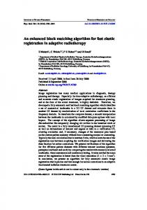
C. Simulated Subjects To further evaluate the accuracy of F-TIMER, we generated 20 simulated deformation fields using the statistical model of deformation (SMD) proposed by Xue et al. [27] to obtain a set of simulated brains with known deformation. Note that SMD was originally proposed for structural images (T1-weighted images in particular). For our case, we generated the set of deformation fields based on a T1 image which was coregistered with the DTI template. One human brain was chosen from the dataset as the template and the 20 simulated deformation fields, which also served as the ground truths, were applied to the template, resulting in 20 simulated human brains. These 20 simulated brains were then registered back onto the template. The deformation fields estimated by the registration were compared with the ground truths. The accuracy of the estimated deformation fields were evaluated and the standard deviation (SD) by the average difference of the two deformation fields, i.e., [4] (25) and (26) where is the Euclidean distance, the number of , the voxels in the brain image volume , and template-to-subject deformation vectors at location of the ground truth deformation field and the estimated deformation field, respectively. By progressively increasing the iteration in both algorithms (8, 16, 24, 32 iterations), we obtained the graphs shown in Fig. 5. Observe from Fig. 5(a) that F-TIMER converges in accuracy much faster than TIMER. In fact, the difference between the first and the last values yielded by F-TIMER is statistically insignif). This validates the fact that the robustness of icant ( our framework permits more confident progression of the registration towards the “optimal” solution. In contrast, TIMER lacks such robust mechanism and it has to be more cautious in each


1200


Fig. 6. Deformation field errors for different regions of the brain.

step, resulting in slower convergence. The lower standard deviations of errors given by F-TIMER, shown in Fig. 5(b) indicate that the deformation field estimation errors are more consistent throughout the brain and are hence less affected by different brain structures. A more detailed region specific summary of the error is provided in Fig. 6. The number of iterations of F-TIMER and TIMER were set so that the two algorithms complete the registration in the same amount of time, i.e., approximately 15 min. The results indicate that F-TIMER performs better than TIMER in all regions.

D. Bending Energy TIMER uses a Gaussian propagation scheme to estimate the dense transformation from the sparse transformations given by a set of sparse landmarks. This might be problematic when the landmarks are unevenly distributed, causing some regions of the brain to be devoid of landmarks. Transformation estimates for these regions can be slow to build up and cause bumpiness due to “holes” in the deformation field. The landmark thinning scheme incorporated in F-TIMER solves part of the problem by ensuring a more even distribution of landmards.



Fig. 7. Bending energy distribution. Comparison were made at the point where both F-TIMER and TIMER gave 1.11 mm.

The TPS interpolation scheme works hand-in-hand to ensure the smoothness of the deformation field, which is important for preserving the anatomical topology of the brain while morphing the image. Fig. 7 shows the bending energy (18) distributions for F-TIMER and TIMER. The distributions are obtained from the average bending energy value at each voxel of the 20 simulated images. For the sake of fairness, we compared F-TIMER and TIMER at the point where both algorithms gave the same deformation error at 1.11 mm. Note that to reach this level of accuracy, TIMER requires approximately 90 min as opposed to 45 min required by F-TIMER. It can be seen from the figure that F-TIMER has a larger fraction of voxels with bending energies distributed close to zero, indicative of the smoothness of the estimated deformation field. It can hence be concluded that F-TIMER is able to achieve higher registration accuracy with a smoother deformation field, and at a shorter amount of time (half of that needed by TIMER). E. Fiber Tracking Using a tractography method known as FACT [28], fiber bundles passing through some regions of interest (ROIs) were tracked, extracted, and compared for quantifying the registration accuracy of F-TIMER. Based on the simulated data generated above, we present here two sets of results. ROIs were selected so a fiber bundle residing in the genu, splenium, and body of the corpus callosum (CC) could be extracted for comparison. The fiber bundles are shown in Fig. 8. Fiber tracking was performed in DTI Studio [28], with the FA start tracking threshold set to 0.25 and the FA stopping threshold set to 0.2. A turning angle of 60 stops the tracking. The same fiber tracking procedure was performed on the F-TIMER registered simulated brains and also the template itself. By comparing the similarity of the fiber tract bundles, we could gauge the effectiveness of F-TIMER in registering the images. The distance of two fiber bundles was then measured in a way similar to that used in [10]. The distance measure is defined as

(27)

1201

Fig. 8. Fiber bundles used for evaluation of F-TIMER. Shown in green, red and yellow are the fiber bundles in the genu, splenium, and body of the corpus callosum, respectively. TABLE II DISTANCES (MM) FOR FIBER BUNDLES PASSING THROUGH DIFFERENT REGIONS OF THE CORPUS CALLOSUM

where is a pairwise distance between fibers and , which in our case, is defined as the mean of the closest distance for every point of two fibers [29]. When two fiber bundles are perfectly aligned, the value returned is zero. This measure approximately establishes anatomic correspondences between points along fibers of different subjects. We compared the performance of F-TIMER with TIMER at its “optimal” number of iterations as was utilized in [13]. The results, shown in Table II, indicate that TIMER, while taking a larger amount of time, does not yield significantly better performance when compared to F-TIMER. Paired -tests performed using individual fiber bundle distances of the 20 subjects do not show significant statistical difference between the two groups of results. F. Mice F-TIMER was also applied to align postnatal mouse brain images. Six images were registered onto a template, and by voxel-wise averaging of the aligned images, an atlas was formed. These mouse images show large changes due to brain growth. There are also tissue contrast changes between mice of earlier and older days, which make the registration difficult. Fig. 9 shows some typical slices in axial, coronal and sagittal views of the color-coded FA maps of the template and the atlas. The sharpness of the atlas indicates that good spatial alignment can be achieved using F-TIMER although it is designed predominantly for human brain images. To further demonstrate the accuracy of the spatial alignment, we extracted the white matter edges of the atlas from its FA map and superimposed them on the corresponding template FA image, as shown in Fig. 10. The


1202


Fig. 9. Axial, coronal, and sagittal views of the template (top panels) and atlas (bottom panels) of the mouse data. The atlas was created by averaging the aligned images. The FA weighted first principal directions are shown in their color coded representations: green for the anterior–posterior direction, blue for the superior–inferior direction, and red for the left–right direction.

Fig. 10. White matter edges generated from the FA map of the atlas overlaid on the template. Three different axial slices are shown. The proper alignment of the edges is indicative of good registration accuracy.

atlas edges agree well with those of the template image and this again confirms the registration accuracy of F-TIMER. IV. CONCLUSION In this paper, we propose an accurate and fast registration algorithm called F-TIMER. F-TIMER extracts distinctive features from a diffusion tensor image—drawing on multiscale tensor regional and boundary information—as automated structural landmarks. Employing these landmarks to minimize an ASSAP related energy function, a smooth, topology preserving, and consistent transformation can be derived. Emperimental results show that F-TIMER can achieve sufficiently good accuracy with a relatively low computation cost. Compared with TIMER, F-TIMER gives comparable accuracy, albeit in a shorter amount of time. With a computation cost of 15 min per 256 256 70 image, the performance of F-TIMER is promising for practical utilization in the clinical scenario. REFERENCES [1] H. Huang, J. Zhang, S. Wakana, W. Zhang, T. Ren, L. Richards, P. Yarowsky, P. Donohue, E. Graham, P. C. M. van Zijl, and S. Mori, “White and gray matter development in human fetal, newborn and pediatric brains,” NeuroImage, vol. 33, no. 1, pp. 27–38, 2006.

[2] A. Lee, N. Lepore, M. Barysheva, Y. Chou, C. Brun, S. Madsen, K. L. McMahon, G. de Zubicaray, M. Meredith, M. Wright, A. Toga, and P. Thompson, “Comparison of fractional and geodesic anisotropy in diffusion tensor images of 90 monozygotic and dizygotic twins,” in ISBI’08, Paris, France, May 14–17, 2008, pp. 943–946. [3] T. Liu, H. Li, K. Wong, A. Tarokh, L. Guo, and S. T. Wong, “Brain tissue segmentation based on DTI data,” NeuroImage, vol. 38, no. 1, pp. 114–123, 2007. [4] J. Yang, D. Shen, C. Misra, X. Wu, S. Resnick, C. Davatzikos, and R. Verma, “Spatial normalization of diffusion tensor images based on anisotropic segmentation,” in SPIE Med. Imag. 2008: Image Process., 2008, vol. 6914, p. 69140L. [5] D. C. Alexander, “An introduction to computational diffusion MRI: The diffusion tensor and beyond,” in Visualization and Processing of Tensor Fields. Berlin, Germany: Springer, 2006, pp. 83–106. [6] H. J. Park, M. Kubicki, M. E. Shenton, A. Guimond, R. W. McCarley, S. E. Maier, R. Kikinis, F. A. Jolesz, and C.-F. Westin, “Spatial normalization of diffusion tensor MRI using multiple channels,” NeuroImage, vol. 20, no. 4, pp. 1995–2009, 2003. [7] C. Goodlett, B. Davis, R. Jean, J. Gilmore, and G. Gerig, “Improved correspondence for DTI population studies via unbiased atlas building,” in Proc. MICCAI’06, 2006, pp. 260–267. [8] J. Ruiz-Alzola, C. F. Westin, S. K. Warfield, C. Alberola, S. Maier, and R. Kikinis, “Nonrigid registration of 3-D tensor medical data,” Med. Image Anal., vol. 6, no. 2, pp. 143–161, 2002. [9] M.-C. Chiang, A. D. Leow, A. D. Klunder, R. A. Dutton, M. Barysheva, S. E. Rose, K. L. McMahon, G. I. de Zubicaray, A. W. Toga, and P. M. Thompson, “Fluid registration of diffusion tensor images using information theory,” IEEE Trans. Med. Imag., vol. 27, no. 4, pp. 442–456, Apr. 2008.



[10] H. Zhang, P. A. Yushkevich, D. C. Alexander, and J. C. Gee, “Deformable registration of diffusion tensor MR images with explicit orientation optimization,” Med. Image Anal., vol. 10, no. 5, pp. 764–785, 2006. [11] B. T. T. Yeo, T. Vercauteren, P. Fillard, X. Pennec, P. Golland, N. Ayache, and O. Clatz, “DTI registration with exact finite-strain differential,” in Proc. IEEE Int. Symp. Biomed. Imag.: From Nano Macro (ISBI’08), Paris, France, May 14–17, 2008, pp. 700–703. [12] T. Vercauteren, X. Pennec, A. Perchant, and N. Ayache, “Non-parametric diffeomorphic image registration with the demons algorithm,” in Proc. Med. Image Computing Computer Assist. Intervent. (MICCAI 07), 2007, vol. 4792, pp. 319–326. [13] P.-T. Yap, G. Wu, H. Zhu, W. Lin, and D. Shen, “TIMER: Tensor image morphing for elastic registration,” NeuroImage, vol. 47, pp. 549–563, 2009. [14] D. Shen and C. Davatzikos, “HAMMER: Heirarchical attribute matching mechanism for elastic registration,” IEEE Trans. Med. Imag., vol. 21, no. 11, pp. 1421–1439, Nov. 2002. [15] G. E. Christensen and H. J. Johnson, “Consistent image registration,” IEEE Trans. Med. Imag., vol. 20, no. 7, pp. 568–582, Jul. 2001. [16] F. L. Bookstein, “Principal warps: Thin-plate splines and the decomposition of deformations,” IEEE Trans. Pattern Anal. Mach. Intell., vol. 11, no. 6, pp. 567–585, Jun. 1989. [17] H. Chui and A. Rangarajan, “A new point matching algorithm for nonrigid registration,” Comput. Vis. Image Understand., vol. 89, no. 2-3, pp. 114–141, 2003. [18] D. Xu, S. Mori, D. Shen, P. C. M. van Zijl, and C. Davatzikos, “Spatial normalization of diffusion tensor fields,” Magn. Reson. Med., vol. 50, no. 1, pp. 175–182, Jul. 2003. [19] J. Yang, D. Shen, C. Davatzikos, and R. Verma, “Diffusion tensor image registration using tensor geometry and orientation features,” in Proc. MICCAI’08, 2008, vol. 11, pp. 905–913.

1203

[20] V. Arsigny, P. Fillard, X. Pennec, and N. Ayache, “Log-Euclidean metrics for fast and simple calculus on diffusion tensors,” Magn. Reson. Med., vol. 56, no. 2, pp. 411–421, 2006. [21] K. Rohr, H. S. Stiehl, R. Sprengel, T. M. Buzug, J. Weese, and M. H. Kuhn, “Landmark-based elastic registration using approximating thinplate splines,” IEEE Trans. Med. Imag., vol. 20, no. 6, pp. 526–534, Jun. 2001. [22] G. Wahba, Spline Models for Observational Data. Philadelphia, PA: SIAM, 1990. [23] G. H. Golub and C. F. V. Loan, Matrix Computations. Baltimore, MD: John Hopkins Univ. Press, 1996. [24] S. Baloch, R. Verma, H. Huang, P. Khurd, S. Clark, P. Yarowsky, T. Abel, S. Mori, and C. Davatzikos, “Quantification of brain maturation and growth patterns in c57bl/6j mice via computational neuroanatomy of diffusion tensor images,” Cerebral Cortex, to be published. [25] R. Verma, S. Mori, D. Shen, P. Yarowsky, and C. Davatzikos, “Spatiotemporal maturation patterns of murine brain quantified via diffusion tensor MRI and deformation-based morphometry,” in Proc. Nat. Acad. Sci., 2005, vol. 102, pp. 6978–6983, 19. [26] M. Jenkinson and S. M. Smith, “A global optimization method for robust affine registration of brain images,” Med. Image Anal., vol. 5, no. 2, pp. 143–156, 2001. [27] Z. Xue, D. Shen, B. Karacali, J. Stern, D. Rottenberg, and C. Davatzikos, “Simulating deformations of MR brain images for validation of atlas-based segmentation and registration algorithms,” NeuroImage, vol. 33, no. 3, pp. 855–866, 2006. [28] H. Jiang, P. C. van Zijl, J. Kim, G. D. Pearlson, and S. Mori, “DtiStudio: Resource program for diffusion tensor computation and fiber bundle tracking,” Comput. Methods Programs Biomed., vol. 81, no. 2, pp. 106–116, Feb. 2006. [29] G. Gerig, S. Gouttard, and I. Corouge, “Analysis of brain white matter via fiber tract modeling,” in Proc. IEEE EMBS, 2004, pp. 4421–4424.
