GPU-Accelerated Elastic 3D Image Registration for Intra-Surgical Applications Daniel Ruijters1,2,3 , Bart M. ter Haar Romeny2 , Paul Suetens3 1
Cardio/Vascular Innovation, Philips Healthcare, the Netherlands,
[email protected], tel: +31 40 2765742 2 Biomedical Engineering, Biomedical Image Analysis, Technische Universiteit Eindhoven, the Netherlands, 3 Universitair Ziekenhuis Gasthuisberg, Medical Image Computing, ESAT/Radiologie, Katholieke Universiteit Leuven, Belgium.
Abstract Local motion within intra-patient biomedical images can be compensated by using elastic image registration. The application of B-spline based elastic registration during interventional treatment is seriously hampered by its considerable computation time. The graphics processing unit (GPU) can be used to accelerate the calculation of such elastic registrations by using its parallel processing power, and by employing the hardwired tri-linear interpolation capabilities in order to efficiently perform the cubic B-spline evaluation. In this article it is shown that the similarity measure and its derivatives also can be calculated on the GPU, using a two pass approach. On average a speedup factor 50 compared to a straight-forward CPU implementation was reached. Key words: Intraoperative brain deformation, Image guided neurosurgery, Non-rigid image registration, Parallel algorithms, Graphics processing unit
Preprint submitted to Computer Methods and Programs in Biomedicine
April 27, 2010
1. Introduction Brain neoplastic disease and arterio-venous malformations (AVM) are pathologies that are frequently treated by neurosurgical resection (Figure 1). In the mentioned applications the surgical resections are rather extensive and cause the leakage of the cerebrospinal fluid followed by brain parenchyma collapse. These phenomena cause the brain to locally deform during treatment. Up to present date commercially available image guidance solutions apply rigid registration during the course of the treatment. The resulting local misalignment, which is inherent to the deformation of the brain and can amount up to 20 millimeters [1, 2], can seriously limit the application of image guided surgery due to the degraded precision. The ultimate solution to overcome these misalignments is the peri-interventional usage of accurate non-rigid registration. The objective of a registration algorithm is to find a spatial mapping between two image datasets. Typically intensity-based registration algorithms consist of a similarity measure, indicating the quality of a given spatial mapping, and an optimization strategy, which iteratively searches the optimum of the similarity measure. The search space consists of the multi-dimensional control variables of the spatial mapping. Non-rigid registration algorithms employ a spatial mapping that allows to model local deformations. Such non-rigid spatial mappings typically are driven by a large number of parameters. In section 2 an overview of the related work is presented. Section 3 introduces the basic mathematics behind the applied elastic registration algorithm. Section 4 describes in detail the steps that are taken to efficiently 2
Figure 1: The surgical resection of an arteriovenous malformation can cause the brain tissue to shift, as is illustrated in this figure. The deformation of the brain can be established by elastically registering a pre- and intra-operative volumetric reconstructions. Pre-operatively planned data can then be mapped on the intra-procedural situation.
3
implement this method on the GPU. Section 5 investigates the performance that can be reached, and compares the GPU implementation to a straightforward and an optimized CPU implementation. Finally, section 6 discusses the usefulness of the accomplished results in neurosurgical applications. 2. Related work Hartkens et al . have shown that it is insufficient to extrapolate the nonrigid deformation by measuring the local displacements of surface of the brain [1]. The displacements have to be tracked for the entire volume of the brain. The group of Warfield et al . has proposed a non-rigid registration method for intra-interventional MR and demonstrated the clinical feasibility [2, 3]. The usage of non-rigid registration during a clinical intervention is seriously hampered by the long calculation times of this type of registration algorithms. The long duration of the calculations can be contributed to the large parameter space of the spatial mapping, given by its many degrees of freedom. The group of Warfield et al . reported that their method, which registered the pre- and intra-interventional data within about 30 seconds on a cluster of 15 workstations, delivered processing times that were considered feasible for image-guided surgical applications [3, 4]. In this article we intend to investigate the viability of obtaining calculation times on a cost-efficient solution by employing the graphics processing unit (GPU) of a single workstation. The vast majority of unconstrained per-voxel spatial mappings are physically impossible or improbable. Penalizing such impossible mappings leads to more robust registration algorithms (i.e. it is more likely that the found 4
mapping corresponds closely to the real deformation) and allows for more efficient algorithms, since fewer solutions need to be probed. There are two basic methods to accomplish this without explicitly identifying the biomedical tissues in the image data; regularization of the per-voxel vector field, or using a deformation field that possesses fewer degrees of freedom than the per-voxel mappings [5]. In this article, we use a cubic B-spline based deformation field, which is sufficiently smooth to model organic elastic displacements of anatomical structures [6]. Furthermore, the local support of the cubic B-spline, together with the reduced number of parameters compared to per-voxel mappings, allows for more efficient calculation times. The computation time of elastic registration can be reduced in two ways; 1) reducing the number of iterations needed to perform a registration, and 2) by reducing the time that is needed per iteration. Kybic and Unser [7] have demonstrated how the number of iterations efficiently can be reduced by using the first order derivatives of the similarity measure, in order to produce a better prediction of the optimum in the optimization strategy. We intend to complement this approach by accelerating the calculations within an iteration, using the vast computation power of modern off-the-shelf Graphical Processing Units (GPU). Though the overall computation power of the GPU nowadays surpasses the power of the CPU [8, 9], its performance does not scale equally well for any type of algorithm. In this article we will demonstrate how the elastic image registration efficiently can be mapped on the GPU, using its hardwired interpolation capabilities and parallel processing power. In the literature there are several publications dealing with GPU-based elastic registration,
5
using a piece-wise linear deformation field [10, 11, 12, 13]. The real human anatomy typically does not deform piecewise linear, and therefore this model can only present an approximation of the real deformation. Higher order models, like cubic B-spline driven deformation fields, offer a smoother deformation field, and therefore posses fewer errors that can be contributed to the interpolation [14]. Some recent publications implement optical flow or demons based non-rigid registration on the GPU [15, 16], unifying the optimization and similarity measure in a combined step. These approaches employ the earlier mentioned regularization of the per-voxel vector field. Also the GPU implementation of B-spline driven deformation in registration using normalized mutual information and normalized cross correlation as similarity measures has been explored [17, 18]. These papers do not use the fast B-spline interpolation method introduced by Sigg and Hadwiger [19], though [17] mentions it as possible future work. In [20] we introduced a GPU-based elastic registration method for 2D images (using fast B-spline interpolation), whereby the similarity measure was obtained in two GPU passes and a third pass on the CPU. In this article we have adapted this approach to 3D image registration, and managed to fit both previous GPU passes in a single pass. Also the part that used to run on the CPU has been brought to the GPU. This is particularly important for volumetric image registration, since this step has become the most time consuming part, see section 5. Furthermore, here we performed a comparison of the GPU approach with a straight-forward and an optimized multi-threaded CPU implementation.
6
3. Computational methods and theory 3.1. Similarity measure In this article we will restrain ourselves to the class of algorithms, in which the similarity measure can be expressed as a sum of contributions per spatial element (pixel for 2D, voxel for 3D, etc.). Sum of Squared Differences (SSD) and Cross-Correlation (CC) are examples of members of this class. This class generally can be written as follows: E=
´ 1 X 1 X ³ ~ e(A(~i), B τ (~i)) = e A(i), B(~τ (~i)) kIk kIk ~i∈I
(1)
~i∈I
Whereby E represents the similarity measure, e the contribution to the similarity measure per spatial element, A the reference image, and B the floating image. ~τ (~i) denotes the deformation of the reference image coordinate system to the floating image coordinate system and B τ is the deformed floating image. ~i ∈ I ⊂ ZN represents the set of N -dimensional discrete spatial positions (i.e. pixel or voxel positions in the image). 3.2. Deformation field The deformation is driven by a set of parameters ~cj . It is this set of parameters that is manipulated by the iterative optimization algorithm. The uniform B-spline driven deformation field then can be described by the following equation [7]: ~τ (~i) = ~i +
X
~cj · β3 (~i/~h − j)
(2)
j∈J
The control points are denoted by ~cj ∈ ZN , and J is the set of parameter indices. Vector ~h represents the spacing of the control points, which we 7
Similarity measure
Contribution per pixel
Derivative
Sum of Squared Differences (SSD)
e(~i) = (A(~i) − B τ (~i))2
δe/δB τ = 2 · (A(~i) − B τ (~i))
e(~i) = A(~i) · B τ (~i)
δe/δB τ = A(~i)
Cross-Correlation (CC)
Table 1: Similarity measures, and their derivative with respect to the deformed image.
require to be integer. Since ~i is added to the sum, the identity deformation corresponds to all control points being zero. β3 (~i) is the N -dimensional tensor product of a uniform cubic B-spline function. 3.3. Derivatives In order to obtain a better prediction of the parameters used in the next iteration, the Jacobian matrix, containing the partial derivatives of the similarity measure to the parameter space δE/δcj,m is required [21], with m denoting the axis. The partial derivative can be decomposed into the following product: ¯ 1 X δe(~i) δB(~x) ¯¯ δτm (~i) δE = δcj,m kIk δB τ (~i) δxm ¯~x=~τ (~i) δcj,m ~
(3)
i∈I
The derivative of the first multiplicand in equation 3 depends on the used similarity measure. In Table 1 the derivatives for SSD and CC are given. In contrary to [7], we do not obtain the derivative δB(~x)/δxm of the deformed floating image analytically. We rather use an image based approach, employing a convolution with Sobel-like kernels. As can be understood from equation 2, the derivative of the deformation field δτm (~i)/δcj,m simply is a constant term: βn (~i/~h − j).
8
4. Program description 4.1. General purpose computing on the GPU The CUDA language [22] is an extension of the C language that makes the massive parallel processing power of the GPU accessible for general purpose programs. The parallel power is harvested by letting the same code, called a ‘kernel’, run in parallel on different pieces of data. The kernels are grouped in blocks, and the blocks are organized in a grid. All kernels in a grid execute the same code, but inter-kernel communication is only possible within a block. A modern GPU has more than hundred parallel processing cores, e.g., the nVidia QuadroFX 5600 possesses 128 processing cores, organized in 16 multiprocessor groups, and has 1.5 GB fast onboard memory. To optimally exploit the processing power of the GPU, there should be many (hundreds) kernels in a grid to keep the processing cores on the GPU filled. The memory on the GPU is organized as smaller amounts of fast register and shared memory, local to each multi-processor, and larger amounts of somewhat slower global memory. Read-only memory can also be declared as fast constant memory or texture memory. The texture memory further has the advantage that it supports very efficient linear interpolation lookups. 4.2. Approach The derivative of the floating image δB(~x)/δxm has to be calculated at ~τ (~i) for all ~i ∈ I. In order to obtain this derivative, the gradient image of the floating image is pre-calculated. It should be noted that this gradient image is static during the optimization process, and therefore needs to be calculated only once for the entire registration procedure. The gradient image can be 9
easily obtained on the GPU by convolving the floating image with Sobel-like derivative kernels of size 3N . 4.3. Similarity measure & derivatives The GPU implementation of the similarity measure and the first order derivatives is illustrated in Figure 2, and works as follows: for every voxel in the reference image a thread is started, and its contribution to the similarity measure and derivatives is calculated. In the thread the corresponding location in the deformed floating data is obtained by adding the cubic B-spline driven deformation offset to the thread’s voxel coordinate, see equation 2. Hereby, we can make efficient use from the fact that a cubic B-spline lookup can be decomposed into 8 linearly weighted interpolations, rather than 64 nearest neighbor lookups, which is much faster on the GPU [19, 23]. When the deformed coordinate has been established, the voxel intensities of the reference and floating datasets are fetched, and the similarity measure contribution of the thread can be established, see equation 1. The gradient of the floating dataset and its intensities are stored in a single texture with four entries per voxel. In this way the interpolated lookup at the deformed coordinate simultaneously yields the intensity and the gradient of the floating data δB(~x)/δxm at this particular location. The derivative of the similarity measure to the control points consists of three multiplicands, see equation 3. Two of those can be established for each GPU thread; the gradient of the floating data δB(~x)/δxm , and the derivative of the similarity measure to the voxel space δe/δB τ . The similarity measure and first order derivatives contributions are stored in an intermediate 3D data array for each thread. The following pseudo CUDA code encapsulates 10
A B
GPU step 1
GPU step 2
Σ
E
Optimizer Figure 2: Block diagram showing the overall dataflow in the algorithm. The first GPU pass takes the reference image A, the floating image B, and the set of deformation coefficients c~j as input. It calculates the contribution to the similarity measure per voxel and the first part of the derivative per voxel. This data is passed to the second GPU pass. This establishes the derivative of the similarity measure to the B-spline coefficients, and passes those to the optimizer. The optimizer determines the new set of B-spline coefficients, and the cycle repeats until the optimum of the similarity measure is found.
the first pass for SSD: __global__ void sim_kernel(float4* output, int3 h) { int3 coord = thread.coord; float3 coordf = make_float3(coord) + 0.5f; float3 offset = interpolate_bspline(deform_coeffs, coordf / h); float3 deform = coordf + offset;
float4 floating = tex3D(flt_img, deform);
//gradient.xyz, image.w
float reference = tex3D(ref_img, coordf);
float diff = reference - floating.w; //gradient, pre-multiplied by derivative of sim. meas. output[coord].xyz = 2 * diff * floating.xyz;
11
1
output[coord].w = diff * diff;
//sim. meas.
}
In the second pass, the first order derivatives δE/δcj,m are calculated by multiplying a subset of the previously stored derivative data with the Bspline weights β3 (~i/~h − j). The B-spline weights are constant, and can be decomposed into a tensor product of three pre-computed 1D arrays of width 4 · hm . The second pass is illustrated by the following pseudo CUDA code: __global__ void coeffs_kernel(float4* output, int3 h) { int3 coord = thread.coord; int3 corner = (coord-2) * h + h/2; int3 extent = 4 * h;
//left-top-front corner
//support of the cubic b-spline
float4 temp = make_float4(0,0,0,0); for (int z = 0; z < extent.z; z++) for (int y = 0; y < extent.y; y++) for (int x = 0; x < extent.x; x++) { float tensor = tex1D(tx, x) * tex1D(ty, y) * tex1D(tz, z); float4 inter = tex3D(intermediate_img, corner+(x,y,z)); temp.xyz += tensor * inter.xyz; temp.w += inter.w; } output[coord] = temp; }
12
(a)
(b)
(c)
(d)
(e) Figure 3: (a) A slice of a cone-beam CT reconstruction of the abdomen taken at the beginning of interventional treatment. (b) The corresponding slice of a reconstruction during the course of the treatment. (c) Subtraction of (a) and (b), whereby dark and light areas indicate the differences between the images. (d) The subtraction image after the elastic registration has been performed. (e) The deformation field illustrated by a checkerboard motif.
13
5. Results Figure 3 illustrated the effect of the described registration algorithm, using real clinical data. The data concerned two cone-beam CT reconstruction of the same volume of interest of 2563 voxels. The registration was performed by the GPU implementation in 14.2 seconds by downsampling the datasets to 1283 voxels using 5 iterations with 83 control points and 30 iterations with 163 control points. As can be seen from the difference images, the deformation of the organs (the liver in this case) is largely corrected by the elastic deformation field. In order to characterize the calculation time of the proposed algorithm, the GPU implementation was compared to a straight-forward single threaded CPU implementation and a multi-threaded SSE optimized CPU version. The cubic interpolation code that forms the basis for the GPU, CPU and SSE implementations can be downloaded from [24]. For all versions we used the approach that is introduced in the previous section, with loop-unrolling applied to the inner for-loop of the second pass. The SSE optimization was also applied to the linear interpolation and the tensor product in the second pass. We used a 2.33 GHz quad-core Intel Xeon with 2 GB memory and an NVIDIA GeForce GTX 260 with 896 MB memory to perform our measurements. As test data we used eight different cone-beam CT datasets of the head of patient with either arterio-venous malformations or aneurysms. The datasets consisted of 2563 isotropic voxels, with voxel sizes ranging from 0.28 mm to 0.40 mm in each direction. The reference and floating data was obtained by deforming each CT dataset according to a B-spline field of 163 uniformly dis14
tributed control points, whereby their magnitude was randomly determined in the range [-8, 8] and some white noise was added to the voxel values. The randomly deformed dataset then served as reference, and the original as floating data. We measured the time to obtain the similarity measure and first order derivatives by performing a quasi-Newton driven optimization in 40 iterations, and averaging the time per iteration. In order to bring the figures in the same range for different dataset sizes (ranging from 323 voxels to 2563 voxels) we divided the time per iteration by the number of voxels in the reference and floating dataset, see Figure 4. The exact numbers representing the time per voxel are given in table 2 and 3 for the SSE and GPU implementations respectively. It can be concluded that, independent from the implementation, the time per voxel depends somewhat on the amount of control points, and not very much on the dataset size. It can be observed that the GPU implementation spends less time per voxel when there are more control points (Figure 2 bottom), which may seem a bit counterintuitive at first glance. The effect can be explained by the fact that there are only few threads running in the second pass when there are few control points, which leads to some parallel processor cores being idle. When the amount of control points increases, the amount of voxels affected by a given control point becomes smaller. Therefore, the processing time per iteration does not necessarily increase. More control points leads to a larger parameter space, which means that typically the optimizer will need more steps to find the optimum, and thus the overall computation time does in fact increase.
15
5400 ns 5200 5000 4800 4600
32³ 64³ 128³ 256³
4400 4200 4000 3800 2³
4³
8³
16³
32³
1600 ns 1400
64³
128³
32³ 64³ 128³ 256³
1200 1000 800 600 400 200 0 2³
4³
8³
16³
32³
64³
400 ns 350
128³
32³ 64³ 128³ 256³
300 250 200 150 100 50 0 2³
4³
8³
16³
32³
64³
128³
Figure 4: The graphs show the amount of time (in nanoseconds) that is spend per voxel, when calculating the similarity measure and first order derivatives for a given transformation. The y-axis indicates the time in nanoseconds, and the x-axis the amount of B-spline transformation control points. The lines in the graphs correspond to different dataset sizes. The top graph shows the measurements for the straight-forward CPU version, the middle graph represents the multi-threaded SSE implementation, and the bottom graph the GPU version. Note that the range of the y-axis differs for the various graphs.
16
23 323
43
793 549
83
163
323
582 607
646
643
1283
643
1351
404 436
458 475
496
1283
1315
391 489
454 442
454
502
2563
1308
378 446
502 528
444
345
Table 2: The amount of time (in nanoseconds) that is spend per voxel, when calculating the similarity measure and first order derivatives using the SSE implementation.
23
43
83
163
323
643
1283
323
354 369
119
97
137
643
302 314
67
59
48
81
1283
243 325
66
67
64
41
71
2563
325 338
133
226
93
60
40
Table 3: The amount of time (in nanoseconds) that is spend per voxel, when calculating the similarity measure and first order derivatives using the GPU implementation.
17
4000 ms 3500 3000 2500 2000 1500 1000 500 0 1
2
3
4
5
6
7
8
Figure 5: The calculation time per iteration (y-axis, in milliseconds) for the SSE implementation, using different amount of threads (x-axis).
On our quad-core machine the multi-threaded SSE algorithm performed best when using four threads (Figure 5), since then the processing resources of the CPU were optimally used with the least amount of thread scheduling overhead. Therefore we used four threads for all our other measurements on the SSE algorithm.s The speedup factor of the GPU version compared to the other two implementations is illustrated in Figures 6 and 7. The boxplots were obtained by comparing the time per iteration for similar datasets sizes and amount of control points. They show the median, and the distribution of the speedup factors. Figures 4, 6 and 7 show that the multi-threaded SSE implementation provides a speedup of approximately a factor 10 over the straight-forward CPU version, whereas the GPU implementation delivers an average speed improvement of of approximately a factor 50. When we dissected the time per iteration into the time used for the first and second pass (Table 4), we discovered that the GPU version spends considerably more time in the second pass than in the first pass.
18
100000 CPU SSE GPU
10000
1000
100
ms
10
1 32³
64³
128³
256³
Figure 6: The calculation time per iteration (y-axis, in milliseconds, logarithmic scale) for different dataset sizes (x-axis, in amount of voxels), using 163 B-spline control points, for the three implementations.
14
12
140
12
10
120
10
100
8
8
80
6 6
60
4
4 2
2
0
0 CPU/SSE
40 20 0
SSE/GPU
CPU/GPU
Figure 7: The boxplots show the speedup factor distribution (y-axis) when comparing the various implementations.
Implementation
Pass 1
Pass 2
Overhead
SSE
536.8 ms
474.2 ms
3.1 ms
GPU
9.6 ms
128.8 ms
1.5 ms
Table 4: Distribution of the time per iteration over the passes, using datasets of 1283 voxels and 163 control points.
19
6. Discussion The application of elastic registration during interventional treatment demands that the registration can be obtained within a limited time frame. The number of iterations that has to be evaluated in the iterative optimization of a similarity measure can be reduced by more accurately predicting the next step towards the optimum, based on the derivative of the similarity measure with respect to the parameter space. In this article we have demonstrated how the similarity measure and its derivative can be calculated on the GPU, using a two pass algorithm. In the first pass the floating image is deformed, using an elastic uniform cubic B-spline deformation field, and the similarity measure and first order derivatives contribution are stored per voxel. The second pass yields the derivative of the similarity measure per control point. The calculation of the derivative was further accelerated by using a static gradient image of the floating image, that was obtained by a convolution with Sobel-like kernels. In this article we focussed on the calculation time of the CPU and GPU implementations of the same basic algorithm. In practise, a good approach has proven to start the registration in low resolution with few control points to find large deformations, and to gradually refine the registration by moving to higher resolutions and more control points [15]. Lets consider e.g. a registration that first performs 20 iterations at a resolution of 643 with 83 control points, then 10 iterations at 1283 with 163 control points, and finally 5 iterations at 2563 with 323 control points. The straight-forward CPU version would take 329 seconds (5.5 minutes) to perform this registration, the multithreaded SSE version costs 31.2 seconds, and the GPU implementation takes 20
7.4 seconds. Five minutes is unacceptable for many interventional and surgical applications, 31.2 seconds becomes an issue when the registration has to be performed multiple times (to compensate for progressively deforming of the brain), while 7.4 seconds is quite acceptable. References [1] T. Hartkens, D. L. G. Hill, A. D. Castellano-Smith, D. J. Hawkes, C. R. Maurer Jr., A. J. Martin, W. A. Hall, H. Liu, C. L. Truwit, Measurement and analysis of brain deformation during neurosurgery, IEEE Trans. Medical Imaging 22 (1) (2003) 82–92. [2] N. Archip, O. Clatz, S. Whalen, D. Kacher, A. Fedorov, A. Kot, N. Chrisochoides, F. Jolesz, A. Golby, P. M. Black, S. K. Warfield, Non-rigid alignment of pre-operative MRI, fMRI, and DT-MRI with intra-operative MRI for enhanced visualization and navigation in imageguided neurosurgery, NeuroImage 35 (2007) 609–624. [3] O. Clatz, H. Delingette, I.-F. Talos, A. J. Golby, R. Kikinis, F. A. Jolesz, N. Ayache, S. K. Warfield, Robust non-rigid registration to capture brain shift from intra-operative MRI, IEEE Trans. Medical Imaging 24 (2005) 1417–1427. [4] N. Chrisochoides, A. Fedorov, A. Kot, N. Archip, P. Black, O. Clatz, A. Golby, R. Kikinis, S. K. Warfield, Toward real-time image guided neurosurgery using distributed and grid computing, in: Proc. ACM/IEEE Conf. Supercomputing, 2006, pp. 37–50.
21
[5] D. Loeckx, Automated nonrigid intra-patient image registration using B-splines, Ph.D. thesis, Katholieke Universiteit Leuven (2006). [6] D. Rueckert, L. I. Sonoda, C. Hayes, D. L. G. Hill, M. O. Leach, D. J. Hawkes, Nonrigid registration using free-form deformations: Application to breast mr images, IEEE Trans. Medical Imaging 18 (8) (1999) 712– 721. [7] J. Kybic, M. Unser, Fast parametric elastic image registration, IEEE Trans. Image Processing 12 (11) (2003) 1427–1442. uger, R. Westermann, Linear algebra operators for GPU implemen[8] J. Kr¨ tation of numerical algorithms, in: International Conference on Computer Graphics and Interactive Techniques, SIGGRAPH’05, 2005, p. 234. uger, A. E. [9] J. D. Owens, D. Luebke, N. Govindaraju, M. Harris, J. Kr¨ Lefohn, T. J. Purcell, A survey of general-purpose computation on graphics hardware, Computer Grphics Forum 26 (1) (2007) 80–113. [10] G. Soza, M. Bauer, P. Hastreiter, C. Nimsky, G. Greiner, Non-rigid registration with use of hardware-based 3D B´ezier functions, in: MICCAI’02, 2002, pp. 549–556. [11] R. Strzodka, M. Droske, M. Rumpf, Image registration by a regularized gradient flow. a streaming implementation in DX9 graphics hardware, J. Computing 73 (4) (2004) 373–389. [12] A. K¨ohn, J. Drexl, F. Ritter, M. K¨onig, H.-O. Peitgen, GPU accelerated 22
registration in two and three dimensions, in: Proc. Bildverarbeitung f¨ ur die Medizin, 2006, pp. 261–265. [13] C. Vetter, C. Guetter, C. Xu, R. Westermann, Non-rigid multi-modal registration on the GPU, in: SPIE Medical Imaging’07, Vol. 6512, 2007. [14] E. H. W. Meijering, Spline interpolation in medical imaging: Comparison with other convolution-based approaches, in: Proc. 10th European signal processing conference (EUPSICO), 2000, pp. 1989–1996. [15] T. Rehman, G. Pryor, J. Melonakos, A. Tannenbaum, Multi-resolution 3D nonrigid registration via optimal mass transport on the GPU, in: Proc. Computational Biomechanics for Medicine-II, MICCAI, 2007, pp. 122–132. ¨ celik, J. D. Owens, J. Xia, S. S. Samant, Fast deformable [16] P. Muyan-Oz¸ registration on the GPU: A CUDA implementation of demons, in: Proc. Computational Science and Its Applications (ICCSA), 2008, pp. 223– 233. [17] M. Teßmann, C. Eisenacher, F. Enders, M. Stamminger, P. Hastreiter, GPU accelerated normalized mutual information and B-spline transformation, in: Eurographics Workshop on Visual Computing for Biomedicine, 2008, pp. 117–124. [18] R. E. Ansorge, S. J. Sawiak, G. B. Williams, Exceptionally fast nonlinear 3D image registration using GPUs, in: IEEE NSS/MIC Workshop on High Performance Medical Imaging (HPMI), 2009.
23
[19] C. Sigg, M. Hadwiger, Fast third-order texture filtering, in: M. Pharr (Ed.), GPU Gems 2: Programming Techniques for High-Performance Graphics and General-Purpose Computation, 2005, pp. 313–329. [20] D. Ruijters, B. M. ter Haar Romeny, P. Suetens, Efficient GPUaccelerated elastic image registration, in: Conf. Biomedical Engineering (BioMed), 2008, pp. 419–424. [21] S. Kabus, T. Netsch, B. Fischer, J. Modersitzki, B-spline registration of 3D images with levenberg-marquardt optimization, in: SPIE Medical Imaging’04, 2004, pp. 304–313. [22] I. Buck, GPU computing: Programming a massively parallel processor, in: Code Generation and Optimization, CGO’07, 2007, p. 17. [23] D. Ruijters, B. M. ter Haar Romeny, P. Suetens, Efficient GPU-based texture interpolation using uniform B-splines, Journal of Graphics Tools 13 (4) (2008) 61–69. [24] D. Ruijters, CUDA cubic B-spline interpolation (CI). URL http://dannyruijters.nl/cubicinterpolation/
24
Summary Brain neoplastic disease and arterio-venous malformations are pathologies that are frequently treated by neurosurgical resection. In the mentioned applications the surgical resections are rather extensive and cause the leakage of the cerebrospinal fluid followed by brain parenchyma collapse. These phenomena cause the brain to locally deform during treatment. The ultimate solution to overcome these misalignments is the peri-interventional usage of accurate non-rigid registration. In this article, we use a cubic B-spline based deformation field, which is sufficiently smooth to model organic elastic displacements of anatomical structures. Furthermore, the local support of the cubic B-spline, together with the reduced number of parameters compared to per-voxel mappings, allows for more efficient calculation times. The similarity measure is restricted to measures that can be expressed as a sum of contributions per spatial element. The proposed approach is fully contained on the GPU, and consists of two passes. In the first pass a thread is started on the GPU for every voxel in the reference image, and its contribution to the similarity measure and derivatives is calculated and stored in an intermediate volumetric array. In the second pass, a thread is run for every B-spline coefficient. For each thread the similarity measure contribution, as well as the first order derivatives of the B-spline deformation parameters, are calculated. In order to characterize the calculation time of the proposed algorithm, the GPU implementation was compared to a straight-forward single threaded CPU implementation and a multi-threaded SSE optimized CPU version. As 25
test data we used eight different cone-beam CT datasets of the head of patient with either arterio-venous malformations or aneurysms. We measured the time to obtain the similarity measure and first order derivatives by performing a quasi-Newton driven optimization in 40 iterations, and averaging the time per iteration. In order to bring the figures in the same range for different dataset sizes we divided the time per iteration by the number of voxels in the datasets. It can be concluded that the time per voxel depends somewhat on the amount of control points, and not very much on the dataset size. On average a speedup factor 50 compared to the straight-forward CPU implementation and a factor 5 with respect to the multi-threaded SSE version was reached. When these performance figures are projected on a realistic calculation scenario, we can conclude that the straight-forward CPU implementation is too slow for habitual application during surgery. The multi-threaded SSE approach is suitable for singular use during the intervention, while the GPU version is considered fast enough for multiple usage to correct for progressive deforming of the treated anatomy. Conflict of interest The authors declare that they have no conflict of interest. No external funding was involved in the execution of the described research.
26