Face Liveness Detection from A Single Image with Sparse ... - PARNEC

Face Liveness Detection from A Single Image with Sparse Low Rank Bilinear Discriminative Model Xiaoyang Tan, Yi Li, Jun Liu and Lin Jiang Dept. of Computer Science and Technology, Nanjing University of Aeronautics and Astronautics, China {x.tan,j.liu}@nuaa.edu.cn

Abstract. Spoofing with photograph or video is one of the most common manner to circumvent a face recognition system. In this paper, we present a real-time and non-intrusive method to address this based on individual images from a generic webcamera. The task is formulated as a binary classification problem, in which, however, the distribution of positive and negative are largely overlapping in the input space, and a suitable representation space is hence of importance. Using the Lambertian model, we propose two strategies to extract the essential information about different surface properties of a live human face or a photograph, in terms of latent samples. Based on these, we develop two new extensions to the sparse logistic regression model which allow quick and accurate spoof detection. Primary experiments on a large photo imposter database show that the proposed method gives preferable detection performance compared to others.

1

Introduction

Biometric techniques, which rely on the inherited biometric traits taken from the user himself for authentication, have gained wide range of applications recently [6]. Unfortunately, once such biometric data is stolen or duplicated, the advantages of biometrics become disadvantages immediately. This situation is most commonly found in a face recognition system, where one or some photos of a valid user can be easily obtained without even physically contacting with him/her, say, through internet downloading or simply capturing them using a camera. A 2D-image based facial recognition system can be easily spoofed by these simple tricks and some poorly-designed systems have even been shown to be fooled by very crude line drawings of a human face [12]. Actually, it is a very challenging task to guard against spoofs based on a static image of a face (c.f ., Fig. 1), while most effort of the current face recognition research has been paid on the ”image matching” part of the system without caring whether the matched face is from a live human or not. Current anti-spoofing methods against photograph or video of a valid user can be categorized based on different criterions, such as the kinds of biometric cues are used, whether additional devices are used, and whether human interaction is needed. A good survey of schemes against photograph spoof can be found in [8] [19]. The most commonly used facial cues include the motion of the facial images such as the blinking of eyes, and the small, involuntary movements of parts of face and head. In [19], an eyeblink-based anti-spoofing method is proposed by integrating a structured prediction

2

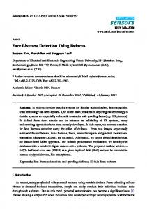
Fig. 1. Do you know which image is captured from a photo? This illustrates the difficulty of detecting photo spoof from a single static image. (Answer: all but the rightmost column are photos.)

method. [10] presents a optimal-flow based method to capture the subtle motion of face images. Although no additional devices are required in these methods, they may encounter difficulties, for example, when a short video of the valid user is displayed or simply shaking the photograph before the camera. [7] gives an interesting example where eye-blinking and some extent of mouth movements can be well simulated using just two photographs. Other commonly used facial cues include the surface texture of the skin and the depth information of the head. In [13], the Fourier analysis is used to capture the frequency distribution of face images of a live human. [20] lists a number of measures that could be used to characterize the optical qualities of skin from face of a live person. If specific devices are available, near infrared images or thermal images can be considered [23]. The 3D information could also be used to provide additional protection against spoof attempts with such devices as 3D cameras or multiple 2D cameras [2]. Besides facial cues, multi-modal information (e.g., voices or gesture etc.), various challenge-response methods (e.g., asking the user to blink, smile or move head ) can also be considered, but these methods need either extra devices or user involvement. Another interesting research against photo spoof is to use a user-specific key to generate a random matrix to distort the face template, so that a ”stolen” face image without the key will be almost of no use [3]. This kind of method, however, mainly focus on the security of biometric templates instead of face liveness detection. Despite the success of the above methods in some cases, non-intrusive methods without extra devices and human involvement are preferable in practice, since they could be easily integrated into an existing face recognition system, where usually only a generic webcam is equipped. 1.1

Motivations and Contributions of This Paper

Partly due to the previously mentioned drawbacks of the facial movement based methods, in this paper we focus on the methods which rely on a single static image to do spoof detection. Such methods can also be directly applied to deal with video spoof or be integrated with a video-based face liveness detection method for better performance. The challenge here, is that the appearance of human face can change drastically due to various illumination conditions and there are also many camera-related factors that

3

may influence the quality of images, which makes it hard to differentiate images from a live person from those from photos (c.f ., Fig. 1). Due to these, simply asking ”what’s in the image (e.g., human skin)” tends to be unreliable. Another strategy is to use various image processing techniques to extract features that highlight the difference between images from live human faces and those from photographs. In [13], a Fourier analysis based method is proposed, in which one third of components with high frequency are heuristically chosen as such features. This method works well when the photo images has low definition and small size. In this paper, the anti-photo spoof problem is formulated as a binary classification problem, thus the statistics from the whole set of images consisting both live human faces and photographs can be fully exploited. This strategy, however, has its own difficulty in that the distributions of positive and negative are largely overlapping in the input space, and a suitable representation space is of importance. Actually, a real human face is different from a face in a photo mainly in two ways: 1) a real face is a 3D object while a photo is 2D by itself; 2) the surface roughness of a real face and a photo is different. These two factors, along with others (such as the definition of photo print and the noise introduced by the camera), usually make different image quality of a real face and a photo face under the same imaging condition (we further assume that both are properly focused). Hence exploiting such information would help to enlarge the intra-class variations between client class and imposter class. For classification, we extended the standard sparse logistic regression classifier both nonlinearly and spatially to improve its generalization capability under the our setting (i.e., high dimensionality and small size samples). It is shown that the nonlinear sparse logistic regression significantly improves the anti-photo spoof performance, while the spatial extension leads to a sparse low rank bilinear logistic regression model, which effectively control the complexity of models without manually specify the target rank beforehand (e.g., in PCA). To evaluate our method, we collected a publicly available large photograph-imposter database containing over 50K photo images from 15 subjects. Preliminary experiments on this database show that the proposed method gives good detection performance, with advantages of realtime testing, non-intrusion and no extra hardware requirement. The paper is organized as follows: in Section 2, we describe in detail the proposed method. Section 3 describes the photograph imposter database and gives the experimental results. Section 4 concludes this paper.

2

The Approach

We formulate the task of detecting photograph spoof as a binary classification problem. However, a simple PCA analysis indicates that there exist large overlapping between the distributions of positive and negative samples (not shown). This indicates that a suitable representation space or measure for determining whether a image arise from a live human is of importance. We do this based on the analysis of Lambertian model [18].

4

2.1

The Face Imaging Model

Suppose that we are given two images, It (x, y) and If (x, y), where It (x, y) is taken from a live human while If (x, y) from an imposter, say, a photograph or a frame of a video clip displayed on a laptop, and (x, y) is the position of each pixel in the image coordinate system. A useful question to ask is: what’s the difference between It (x, y) and If (x, y) under the same illumination condition 1 ? We examine this under the Lambertian reflectance assumption, where the face surface is modeled as an ideal diffuse reflectors, hence reflecting light according to Lambert’s cosine law [18]. In other words, the intensity of a face image I(x, y) is described as I(x, y) = fc (x, y)ρ(x, y)Alight cos θ,

(1)

where fc (x, y) term depends on the underlying camera, Alight is the intensity of the incoming light at a particular wavelength. The ρ(x, y) term is the reflectance coefficient, which represents the diffuse reflectivity of the surface at that wavelength. The cos θ = n · s is the angle between the surface normal n and the incoming light ray s. First we assume that fc (x, y) is a constant. This is reasonable for many webcams. Then the client image It (x, y) and imposter image If (x, y) can be respectively expressed as, It (x, y) = ρt (x, y)Alight (nt · s), If (x, y) = ρf (x, y)Alight (nf · s).

(2) (3)

These equations say that if under the same lighting conditions (i.e., Alight , s terms are fixed), the differences between the two images can be made evident by comparing their surface properties, i.e., the surface reflectance property ρt \ρf , and the surface normal nt \nf at that point. Intuitively this is feasible since the human skin and a photograph (or the Laptop which is replaying a video clip) are made of different materials and the smoothness of their surfaces are different as well. For example, some previous work [13] uses the high frequency components of the given image to identify possible spoof. This method can be considered as a rough way to approximate the ρ value, but the information from n is lost. For the sake of robustness under various conditions (e.g., against high-definition photograph spoof), exploiting full information from a given image is essential. To do this, one can write the above equations as follows, It (x, y) = ρt (x, y)A(nt · s) , ρt (x, y)µt (x, y) If (x, y) = ρf (x, y)A(nf · s) , ρf (x, y)µf (x, y)

(4) (5)

where we denote µ(x, y) = Alight (n · s), which is a function of the surface normal n. Hence the information we are interested in are actually encoded in the functional ρ(x, y) and µ(x, y). Although we usually cannot watch the behavior of these functionals directly, we may estimate them if a series of m samples of xiρ = ρi (x, y) and xiµ = µi (x, y), i = 1, 2, . . . , m, are available. We will call these samples ”latent samples” since they are hidden by themselves, and we need a method to derive them. 1

This assumption will be largely relaxed later.

5

2.2

Deriving Latent Samples

In this section we present two methods to derive the latent samples for our discriminative model. Variational Retinex-based Method. To solve (4) or (5), one has to decompose a given face image into reflectance part ρ(x, y) and illuminance part µ(x, y), which is exactly what most illumination invariant face recognition method does. Note that, however, for illumination invariant face recognition, once the albedo of a face image is obtained, the illuminance part is usually discarded. But in our case, the illuminance part is useful since it contains information about the surface normal (c.f . (4)). In particular, for a photograph, the surface normal is mostly constant hence the lighting factor s will actually be dominant in various µf (x, y) images. While for a real face, both n and s will count in µt (x, y). This nature of imaging variability turns out providing useful discriminative information about whether a µ(x, y) image is from a 3D object or not. Here we prefer a type of variational Retinex approach, in which the illuminance µ(x, y) is first principally sought within the total variational framework and the albedo ρ(x, y) is then estimated through Land’s Retinex formula [11]. Typical methods in this line include the anisotropic smoothing method by Gross et al. [4] and Logarithmic Total Variation (LTV) smoothing by Chen et al. [1]. In this work we take the Logarithmic Total Variation (LTV) method for experiments, where a plausible illumination image µ(x, y) is estimated by minimizing a functional combining smoothness and fidelity terms: Z µ = arg min k∇µk1 + λ |I − µ| (6) image

where λ is the data fidelity parameter (set to 0.5 in this work). Once the µ is obtained, we estimate ρ through log(ρ(x, y)) = log(I(x, y) + 1) − log(µ(x, y) + 1) using Land’s Retinex formula [11] (c.f ., (4)). Fig. 2 gives some illustration of the ρ image and µ image decomposed in this manner, from a client image and a imposter image, respectively. It can be observed that the texture of µf image from a photo is less rich than µt from a real face as expected. Difference of Gaussian (DoG)-based Method. Another method is based on the intuitive idea that the image of a photograph taken through a webcam is essentially an image of a real face but passes through the camera system twice and the printing system once. This means that compared to an image of a real human, the imposter image tends to be more seriously distorted by the imaging system and hence has lower image quality (i.e., missing more high frequency details) under the same imaging conditions. We may exploit this characteristic to distinguish an imposter image and a client image. In particular, we do this by analyzing the 2D Fourier spectra similar to [13]. But instead of using very high frequency band which maybe too noisy, we try to exploit the difference of image variability in the high-middle band. This is done through Difference of Gaussian (DoG) filtering which is essentially a bandpass filter and has successfully been applied to remove lighting variations in face images [25]. To keep as much detail as possible without introducing noise or aliasing, we take a quite narrow inner (smaller) Gaussian (σ0 ≤ 1), while the outer one might have σ1 of 1-2 pixels to filter out misleading low spatial frequency information. In other words, by using this preprocessing

6

Fig. 2. Illustration of the latent samples derived for a client image (top row) and an imposter image (bottom row): from left to right, 1) the raw image; 2) the µ image estimated with LTV; 3) the ρ image estimated with LTV; 4) the centered Fourier spectra of the raw image; 4) the centered Fourier spectra of the image filtered with DoG.

procedure, when comparing two images, we can focus more on their major part of image information without being confused by non-relevant information. In this work, we use σ0 = 0.5 and σ1 = 1.0 by default. Fig. 2 gives some illustration of two images (one client image and one imposter image) and their respective Fourier spectra with/without DoG filtering. It can be observed that the DoG filter cleans the noise in the high frequency areas. In addition, the client image contains richer horizontal components in the high frequency areas than the imposter image, while the two images’ respective distributions of components in various orientations are different in the middle band. Hence compared to the previous LTV-based method, the appearance variations of face images are emphasized here. 2.3

Classification

In the most simple case where the photos are taken under the same lighting condition with real faces (i.e., sf = sf = s), we have µf (x, y)\µt (x, y) = (nf · s)\(nt · s). One can see that it is the surface norms nt and nf that dominate the ratio. This implies that one can try to first capture a real face for that specific lighting scenario then used it as reference to reject possible photo spoofing under that scenario. In more general case where the st and sf are different, one strategy is to first learn K most common lighting settings where photo spoofing may happen from training samples, using such method as Singular Value Decomposition [28]. Denote these settings as a lighting matrix S ∈ R3×K . One can use this S to reconstruct any µ ∈ RD image such that k µ − N Sv k is minimized, where N ∈ RD×3 is the surface normal matrix to be estimated, v ∈ RK is the reconstruction coefficient. The object function can be optimized by coordinate descent method. After this, the reconstruction coefficient v can be used as input to a classifier. But things become more complicated if we take the illumination distribution of each photo itself into consideration. This lighting distribution is independent with the current lighting setting, and according to Lambertian model, it should go into the albedo part but (depending on the setting of λ ) the LTV decomposition (c.f ., (6)) often allow a significant amount of fine scene texture to leak into µ, thus making the distribution of µ

7

become rather nonlinear. Therefore, in this work we learn a classifier directly through the obtained latent training samples without further feature extraction. In particular we adopted the sparse logistic regression model and extend it in two ways such that it may better fit the problem at hand. Sparse Logistic Regression. Let x ∈ Rn denote a sample, and y ∈ {−1, 1} be the associated (binary) class label (we define imposter image as +1, client image -1). Logistic regression model is given by: Prob(y|x) =

1 , 1 + exp(−y(wT x + b))

(7)

where Prob(y|x) is the conditional probability of class y = 1, given the sample x, w ∈ Rn is the weight vector, and b ∈ R is the intercept. Suppose that we are given a set n of m training data {xi , yi }m i=1 (c.f ., Sec. 2.2), where xi ∈ R denotes the i-th sample and yi ∈ {−1, +1} denotes the corresponding class label. The likelihood function Qm associated with these m samples is defined as i=1 Prob(yi |xi ). The negative of the log-likelihood function is called the (empirical) logistic loss, and the average logistic loss is defined as: loss(w, b) = −

m Y 1 log Prob(yi |xi ) m i=1 m

(8)

1 X = log(1 + exp(−yi (wT xi + b))), m i=1 which is a smooth and convex function. We can determine w and b by minimizing the average logistic loss: minw,b loss(w, b), leading to a smooth convex optimization problem. The sparse logistic regression [9, 14] add a `1 -norm regularization to the loss to avoid overfitting, i.e., minw,b loss(w, b) + λkwk1 . The major characteristic of this is that it enforces a sparse solution which is desirable for our application. In addition, there are quite a few efficient solvers for optimizing this problem, e.g., l1-log [9] and SLEP [14]. In this paper, we propose to make use of the SLEP package [16], as it enjoys the optimal convergence rate and works efficiently for large scale data. Sparse Low Rank Bilinear Logistic Regression. To exploit the spatial property of images, we can directly operate on the two-dimensional representation of images. The goal is to learn a ”low-rank” projection matrix, or equivalently a ”low-rank” bilinear function: fL,R (X) = tr(LT XRT ) = tr((LR)T X), (9) where X ∈ Rr×c , L ∈ Rr×c , R ∈ Rc×c , and r and c denote the number of rows and columns of the image X, respectively. Denote W = LR ∈ Rr×c , we can rewrite (9) as fL,R (X) = tr(W T X) = hvec(W ), vec(X)i, leading to the traditional onedimensional (concatenated) linear function. However, directly learning (9) from a set of training samples can leads to overfitting, especially when m, the number of training samples is less than p = r × c, the dimensionality. One standard technique is to add some penalty to control the complexity of the learned W = LR ∈ Rr×c . In this study, we impose the assumption that W is

8

a “low-rank” projection matrix. Given a set of training samples {Xi , yi }ni=1 , one way to compute W = LR is to optimize: min loss(L, R) + λ × rank(LR), L,R

(10)

where loss(L, R) is a given loss function defined over the training samples, e.g., the logistic loss (8). However, rank(LR) is nonconvex, and (10) is NP-hard. So instead we propose to compute L and R via min loss(L, R) + λ1 kLk2,1 + λ2 kRk2,1 . L,R

(11)

where k · k2,1 is the `(2, 1)-norm of a matrix defined as the sum of the `2 length of each column of this matrix. With appropriate parameters, (11) shall force a solution where many rows of L and R are exactly zero, so that L and R are “low-rank”. As rank(W ) ≤ max(rank(L), rank(R)), the obtained W = LR is also low-rank. To optimize (11), we apply the block coordinate descent. That is to say, we first fix R to obtain L via minL φR (L) + λ1 kLk2,1 , where φR (L) is a convex and smooth function with regard to L under given R. Similarly, we compute R under given L via minR ψL (R) + λ2 kRk2,1 . And this process is repeated until convergence. A common practice is to terminate the program after the change of L and R (measured in the Frobenius norm) in the adjacent iterations is below a small value (1e-6 in the paper). This model has several new features: 1) In contrasted with the existing low rank bilinear discriminative method (e.g., [21]), the rank needs not to be pre-specified, but tuned via λ1 and λ2 2 ; 2) The “low-rank” projection matrix W is obtained the computationally efficient penalty k ·k2,1 -norm without Singular Value Decomposition as needed by the trace-norm or nuclear norm; 3) Recall fL,R (X) = tr(LT XRT ), LT have many columns that are exactly zero, thus being able to discarding certain columns in Xi ’s. Physically, this parameter matrix contains sets of learned discriminative filters for each thin strip of the face image, thus encoding spatial information. Nonlinear Model via Empirical Mapping. In a second extension to the sparse logistic regression model, we make use of the explicit empirical mapping defined over the m training samples to transform them into the features space via the kernel mapping φ : ˜ = φ(x), we define x → F , thus we have F = Rm . Let x x ˜j = kernel(x, xj ), j = 1, 2, . . . , m,

(12)

where kernel(·, ·) is a given kernel function, e.g., the Gaussian kernel (c.f . [5] for a good account on this in the context of RBF network). With the transformed training data {˜ xi , yi }m i=1 , we can apply the sparse logistic regression discussed before for constructing a sparse model. One way to look at this model is that it can be thought of as a nonparametric probabilistic model since its number of parameters grows with the sample size while its 2

In the experiments, we follow a two-step procedure suggested in [17] to set the values of these two parameters, where a small value (1e-6) is first set for both lambda’s then those coefficients with small absolute values are removed off.

9

Fig. 3. Illustration of the samples from the database. In each column (from top to bottom) samples are respectively from session 1, session 2 and session 3. In each row, the left pair are from a live human and the right from a photo. Note that it contains various appearance changes commonly encountered by a face recognition system (e.g., sex, illumination, with/without glasses). All original images in the database are color pictures with the same definition of 640×480 pixels.

complexity is controlled by the `1 -norm prior. This characteristic is shared by many sparse nonlinear discriminative models in literatures, such as probabilistic Support Vector Machine (pSVM, [22]), Relevance Vector Machine (RVM, [26]) and Import Vector Machine (IVM, [29]). The major merit of our model, however, lies in its simplicity and its flexibility to allow a straightforward application of any efficient solver dealing with usual sparse logistic regression problem, without any modification on them. Take the SLEP used here for example, its computational complexity is O(m2 )[15], compared to O(m3 ) for pSVM, O((m + 1)3 ) for RVM and O(m2 q 2 ) for IVM (q is the number of import points).

3

Experiments

3.1

Database

We constructed a publicly available photograph imposter database3 using a generic cheap webcam bought from an electronic market. We collected this database in three sessions with about 2 weeks interval between two sessions, and the place and illumination conditions of each session are different as well. Altogether 15 subjects (numbered from 1 to 15)4 were invited to attend in this work. In each session, we captured the images of both live subjects and their photographs. Some sample images from the three sessions are given in Fig. 3. In particular, for each subject in each session, we used the webcam to capture a series of their face images (with frame rate 20fps and 500 images for each subject). Dur3 4

http://parnec.nuaa.edu.cn/xtan/data/NUAAImposterDB.html Since the major goal of this work is to distinguish a real face from a photograph, rather than differentiate different people as the case of usual face recognition, the requirement of large number of subjects is less demanding compared to the richness of variations contained in the datasets.

10

Fig. 4. Illustration of different photo-attacks (from left to right) : (1) move the photo horizontally, vertically, back and front; (2) rotate the photo in depth along the vertical axis; (3) the same as (2) but along the horizontal axis; (4) bend the photo inward and outward along the vertical axis; (5) the same as (4) but along the horizontal axis.

ing image capturing, each subject was asked to look at the webcam frontally and with neutral expression and no apparent movements such as eyeblink or head movement. In other words, we try to make a live human look like a photo as much as possible (vice versa for photograph). Some examples of the captured images are illustrated in Fig. 3 (left column). To collect photograph samples, we first took a high definition photo for each subject using a usual Canon camera in a way that the face area should take at least 2/3 of the whole area of the photograph. We then developed the photos in two ways. The first is to use the traditional method to print them on a photographic paper with the common size of 6.8cm × 10.2cm (small) and 8.9cm × 12.7cm (bigger), respectively. In the other way, we print each photo on a 70g A4 paper using a usual color HP printer. Based on these, three categories of the photo-attacks are simulated before the webcam, in a way similar to [19], as shown in Fig. 4.

3.2

Settings and Performance Measure

To evaluate our methods, we first constructed a training set and a test set from the photo imposter database, both of which contain a number of client images and imposter images. The training set is constructed using the images from the first two sessions and the test set from the third session. In particular, the training set contains 889 images from the first session and 854 images from the second session and all the available subjects in the two sessions are involved.Hence we got 1743 images from 9 subjects as valid biometric trait. For the imposter images of the training set, we respectively selected 855 and 893 images from the first and the second sessions of the photograph set, hence we got 1748 imposter images in all. The test set contains 3362 images from live humans selected from session 3 and 5761 images from photos selected from session 3 as well. Table 1 gives some statistics of this. Note that there is no overlapping between the training set and the test set. In addition, some subjects in the test set are not appeared in the training set,which increases the difficulty of the problem.

11 Table 1. The number of images in the training set and test set. Session1 session2 session3 Total Training Set Client 889 854 0 1,743 Imposter 855 893 0 1,748 Total 1,744 1,747 0 3,491 Test Set Client 0 0 3,362 3,362 Imposter 0 0 5,761 5,761 Total 0 0 9,123 9,123

All the images then undergo the same geometric normalization prior to analysis: face detected and cropped using our own Viola-Jones detector [27], rigid scaling and image rotation to place the centers of the two eyes at fixed positions, using the eye coordinates output from a eye localizer [24]; image cropping to 64 × 64 pixels and conversion to 8 bit gray-scale images. 3.3

Experimental Results

Fig. 5 (Left) compares the overall performance using sparse (linear) logistic regression (SLR) with different types of input. This figure shows that the raw image (RAW) and the µ image estimated with LTV [1] (LTVu) give much worse result than the other three, i.e., ρ image (LTVp), DoG filtered image (DoG) and one third of the highest frequency components in [13] (HF) (the fusion of LTVp and LTVu doesn’t make big difference here and is not shown). This indicates that although the LTVu images are useful as analyzed before, their discriminative capability can not be exploited using a linear classifier. On the other hand, the improved performance given by both LTVp and DoG shows that these two representations helps to increase the separability of the sample space. In addition, they both outperform HF in terms of AUC value5 (respectively 0.78, 0.75 and 0.69 for the three), showing that the highest frequency components are not stable enough due to the influence of noise or aliasing in these areas. Due to the unsatisfying performance of raw gray-scale image and being rarely directly used in practice, we don’t pursue this method any more in the following experiments. To examine the effectiveness of the proposed sparse low rank bilinear logistic regression (SLRBLR), we conducted a series of experiment on the DoG images (we don’t repeat the experiment on the LTV images due to their highly nonlinear distribution). We also tested a specific case of (11) named SLRBLRr1, by setting L ∈ Rr×1 , R ∈ Rc×1 , i.e., rank(W ) = 1. The results are shown in Fig. 5 (Right), which shows that the sparse low rank bilinear models (with AUC value 0.92 for SLRBLR and 0.95 for SLRBLRr1) significant improve the performance upon the standard sparse logistic regression model (with AUC value 0.75). 5

AUC: Area Under the ROC Curve, the larger the better.

12 LTVp

LTVu

DoG

HF

SLRBLRr1 1

0.9

0.9

0.8

0.8

0.7

0.7 True positive rate

True positive rate

RAW 1

0.6 0.5 0.4

0.5 0.4 0.3

0.2

0.2

0.1

0.1

0

0.1

0.2

0.3

0.4 0.5 0.6 False positive rate

0.7

0.8

0.9

0

1

SLR

0.6

0.3

0

SLRBLR

0

0.1

0.2

0.3

0.4 0.5 0.6 False positive rate

0.7

0.8

0.9

1

Fig. 5. (Left) Detection performance with various input features using the sparse (linear) logistic regression (SLR); (Right) Performance on the DoG images with various sparse linear discriminative model. LTVp

LTVu

LTVfused

DoG

HF SLR

1

SNLR

SVM

100

0.9 90

0.8 80

0.7

Accuracy (%)

True positive rate

70

0.6 0.5 0.4

60 50 40

0.3 30

0.2 20

0.1 10

0

0

0.1

0.2

0.3

0.4 0.5 0.6 False positive rate

0.7

0.8

0.9

1

0

LTVp

LTVu

LTVfused

DOG

HF

Fig. 6. (Left) Detection performance with various input features using the sparse nonlinear logistic regression. (Right) Comparison of detection rate (%) using various classification methods and input features.

Fig. 6 (Left) gives the results if we replace the linear classifier with a nonlinear one, i.e., our sparse nonlinear logistic regression (SNLR). This shows big performance improvement upon previous. In particular, the performance of LTVu drastically improves from 0.22 to 0.92 (in terms of AUC), which verify the effectiveness of nonlinear decision boundary. Actually, by combining the LTVp and LTVu, we get further performance improvement (to 0.94). Compared to others, the ROC curve of the DoG image shows a very rapid rising tendency from the very beginning of the horizontal axis. Hence it is considered the best option for use in practice among the methods compared here. Fig. 6 (Right) shows the best overall classification accuracy of different types of input image tested respectively using sparse linear logistic regression (SLR [14]), sparse nonlinear logistic regression (SNLR) and probabilistic support vector machine (SVM [22]). We obtained this by evaluating the proportion of correctly labeled samples (either client

13

or imposter) among the whole 9,123 test set by properly thresholding the output of each discriminative model. The figure shows that the components in the middle frequency (DoG) outperforms those in the one-third of the highest frequency (HF) by removing both the noise/alias in high frequency area and the misleading spatial information in low frequency area. In contrast, the Fourier spectra analysis method in [13] gives a classification rate of 76.7% (not shown in the figure) - about 10% lower than that of DoG. As for the image decomposition method, we see that both the albedo (LTVp) and structure (LTVu) part contribute to the discriminative capability of the system, especially when a nonlinear model is used. Combining them slightly improves the performance.

4

Conclusions

In this work, we present a novel method for liveness detection against photo spoofing in face recognition. We investigate the different nature of imaging variability from a live human or a photograph based on the analysis of Lambertian model, which leads to a new strategy to exploit the information contained in the given image. We show that some current illumination-invariant face recognition algorithm can be modified to collect the needed latent samples, which allows us to learn a sparse nonlinear/bilinear discriminative model to distinguish the inherent surface properties of a photograph and a real human face. Experiments on a large photo imposter database show that the proposed method gives promising photo spoof detection performance, with advantages of realtime testing, non-intrusion and no extra hardware requirement. Learning the surface properties of object through samples is an classical open problem in computer vision. Although there are lots of related work in the field of texture analysis, their goal is different from ours. We believe that our work is the first one trying to use the learning technique to distinguish whether a given static image is from a live human or not. We are currently investigating the possibility to integrate various texture descriptors to further improve the performance.

Acknowledgement Thank anonymous reviewers for their valuable comments. This research was supported by the National Science Foundation of China (60773060, 60905035), the Jiangsu Science Foundation (BK2009369) and the Project sponsored by SRF for ROCS, SEM.

References [1] Chen, T., Yin, W., Zhou, X., Comaniciu, D., Huang, T.: Total variation models for variable lighting face recognition. IEEE TPAMI 28(9), 1519–1524 (2006) [2] Fladsrud, T.: Face recognition in a border control environment. Tech. rep. (2005) [3] Goh, A.: Random multispace quantization as an analytic mechanism for biohashing of biometric and random identity inputs. IEEE TPAMI. 28(12), 1892–1901 (2006) [4] Gross, R., Brajovic, V.: An image preprocessing algorithm for illumination invariant face recognition. In: AVBPA. pp. 10–18 (2003) [5] Haykin, S.: Neural Networks: A Comprehensive Foundation. Prentice Hall (1999)

14 [6] Jain, A.K., Flynn, P., Ross, A.A.: Handbook of Biometrics. Springer-Verlag New York, Inc. (2007) [7] Joshi, T., Dey, S., Samanta, D.: Multimodal biometrics: state of the art in fusion techniques. Int. J. Biometrics 1(4), 393–417 (2009) [8] K.Nixon, V.Aimale, R.Rowe: Spoof detection schemes. In: Handbook of Biometrics. pp. 403–423 (2008) [9] Koh, K., Kim, S., Boyd, S.: An interior-point method for large-scale l1-regularized logistic regression. JMLR 8, 1519–1555 (2007) [10] Kollreider, K., Fronthaler, H., Bigun, J.: Non-intrusive liveness detection by face images. Image Vision Comput. 27(3), 233–244 (2009) [11] LAND, E.H., McCANN, J.J.: Lightness and retinex theory. J. Opt. Soc. Am. 61(1), 1–11 (1971) [12] Lewis, M., Statham, P.: CESG biometric security capablilities programme: Method, results and research challenges. In: Biometrics Consortiumn Conference (2004) [13] Li, J., Wang, Y., Tan, T., A.K.Jain: Live face detection based on the analysis of fourier spectra. In: SPIE. pp. 296–303 (2004) [14] Liu, J., Chen, J., Ye, J.: Large-scale sparse logistic regression. In: ACM SIGKDD International Conference On Knowledge Discovery and Data Mining (2009) [15] Liu, J., Ji, S., Ye, J.: Multi-task feature learning via efficient `2,1 -norm minimization. In: Uncertainty in Artificial Intelligence (2009) [16] Liu, J., Ji, S., Ye, J.: SLEP: Sparse Learning with Efficient Projections. Arizona State University (2009), http://www.public.asu.edu/˜jye02/Software/SLEP [17] Meinshausen, N., Yu, B.: Lasso-type recovery of sparse representations for highdimensional data. Annals of Statistics pp. 246–270 (2009) [18] Oren, M., Nayar, S.: Generalization of the lambertian model and implications for machine vision. IJCV 14(3), 227–251 (1995) [19] Pan, G., Wu, Z., Sun, L.: Liveness detection for face recognition. In: Recent Advances in Face Recognition. pp. 236–252 (2008) [20] Parziale, G., Dittmann, J., Tistarelli, M.: Analysis and evaluation of alternatives and advanced solutions for system elements. In: BioSecure (2005) [21] Pirsiavash, H., Ramanan, D., Fowlkes, C.: Bilinear classifiers for visual recognition. In: NIPS, pp. 1482–1490 (2009) [22] Platt, J.C.: Probabilistic outputs for support vector machines and comparisions to regularized likelihood methods. In: Advances in Large Margin Classifiers, pp. 61–74. MIT Press (1999) [23] Socolinsky, D.A., Selinger, A., Neuheisel, J.D.: Face recognition with visible and thermal infrared imagery. Comput. Vis. Image Underst. 91(1-2), 72–114 (2003) [24] Tan, X., Song, F., Zhou, Z.H., Chen, S.: Enhanced pictorial structures for precise eye localization under uncontrolled conditions. In: CVPR. pp. 1621–1628 (2009) [25] Tan, X., Triggs, B.: Enhanced local texture feature sets for face recognition under difficult lighting conditions. IEEE Transactions on Image Processing 19(6), 1635–1650 (2010) [26] Tipping, M.E.: The relevance vector machine. In: NIPS 12, pp. 652–658 (2000) [27] Viola, P., Jones, M.J.: Robust real-time face detection. IJCV 57(2), 137–154 (2004) [28] Yuille, A.L., Snow, D., Epstein, R., Belhumeur, P.N.: Determining generative models of objects under varying illumination: Shape and albedo from multiple images using svd and integrability. IJCV 35(3), 203–222 (1999) [29] Zhu, J., Hastie, T.: Kernel logistic regression and the import vector machine. In: J. Compu. & Graph. Stat. pp. 1081–1088 (2001)